Mining Behavioral Groups in Large Wireless LANs

Abstract

One vision of future wireless networks is that they will be deeply integrated and embedded in our lives and will involve the use of personalized mobile devices. User behavior in such networks is bound to affect the network performance. It is imperative to study and characterize the fundamental structure of wireless user behavior in order to model, manage, leverage and design efficient mobile networks. It is also important to make such study as realistic as possible, based on extensive measurements collected from existing deployed wireless networks.

In this study, using our systematic TRACE approach, we analyze wireless users’ behavioral patterns by extensively mining wireless network logs from two major university campuses. We represent the data using location preference vectors, and utilize unsupervised learning (clustering) to classify trends in user behavior using novel similarity metrics. Matrix decomposition techniques are used to identify (and differentiate between) major patterns. While our findings validate intuitive repetitive behavioral trends and user grouping, it is surprising to find the qualitative commonalities of user behaviors from the two universities. We discover multi-modal user behavior for more than $60\%$ of the users, and there are hundreds of distinct groups with unique behavioral patterns in both campuses. The sizes of the major groups follow a power-law distribution. Our methods and findings provide an essential step towards network management and behavior-aware network protocols and applications, to name a few.

I Introduction

In recent years, we have witnessed the mass deployments of portable computing and communication devices (e.g., cellphones, laptops, PDAs) and wireless communication infrastructures. As the adoption of these technologies becomes an inseparable part of our lives, we envision that future usage of mobile devices and services will be highly personalized. Users will incorporate these new technologies into their daily lives, and the way they use new devices and services will reflect their personality and lifestyle truthfully. To understand its impact, we believe that there is a pressing need to go beyond the technological perspective and capture and understand the user behavioral patterns as users adopt the new technology. This understanding will also play a crucial role in solving a multitude of technical issues, ranging from better network management to designing of behavior-aware protocols, services, and user models.

Consider wireless LANs (WLANs) on university campuses as an example. One could imagine the major work places (e.g., offices and classrooms) and the informational hubs (e.g., libraries and computer centers) would dominate users’ behavioral patterns in terms of network usage. However, as the WLAN deployments prevail, the location from where people access information is bound to change. While the traditional ”hot spots” still play an important role, we can expect users to display diverse behavioral patterns that reflect their personal preferences (e.g., A small group may prefer to work at a coffee shop), as these wireless devices become tiny and personalized. We need to understand such behavioral patterns to better characterize the users within a social context. The technique to discover such patterns from collected data is the focus of our paper.

In this paper we take a first step towards understanding and characterizing the structure of behavioral patterns of users within large WLANs. We develop methods to identify groups of users that demonstrate similar and coherent behavioral pattern. This is important for several reasons: (1) From the network management perspective, it helps us to understand the potential interplay of the user groups with the network operation and reveals insight previously unavailable by looking at the mere aggregate network statistics. (2) From the application or service perspective, the groups identify different existing major behavioral modes in the network, and, hence, can be potentially utilized to identify targets for group-aware services. (3) From a social sciences perspective, the results unravel the relationships between users (i.e., their ”closeness” in terms of network usage behavior) when they incorporate wireless mobile devices as an inseparable part of their daily lives.

We apply our analysis framework on long-term WLAN traces obtained from two university campuses[13, 14] across the coasts of USA. We represent a user’s behavioral features by constructing the normalized association matrix to which we apply our analysis. While the applicability of our methods is not specific to WLANs, these are the most extensive wireless user behavioral traces available today. Although this is not the first study of these WLAN traces, our unique focus is on user groups across campuses while most of the previous studies focus on individual user behavior models or aggregate statistics within one campus. We leverage unsupervised learning (i.e., clustering) techniques [1] to determine groups of users displaying similar behavior. While clustering has been widely-applied in other areas, the main contribution of the paper is to construct proper representations for our data sets and design novel distance metrics between users. These two aspects are fundamental in the application of clustering techniques and determine the quality of the results we obtain. The key challenge in designing a good distance metric is to accurately and succinctly summarize the trends in the data, so the distances are not influenced by noise and can be evaluated efficiently. We show that a singular-value decomposition (SVD) based scheme not only provides the best summary of the data, but also leads to a distance metric that is robust to noise and computationally efficient. Furthermore, we validate our methods and explain its significance.

We find the following common trends from the two diverse datasets: (1) More than $60\%$ of the WLAN users display multi-modal behavior (their behavior can be decomposed into multiple modes or types) in the long run. However, for many users the most dominant behavioral mode is much stronger than the rest. This leads to efficient summaries of their behavioral patterns. With SVD, we can capture more than $90\%$ of the power in the association patterns with just five components. (2) Current university WLANs consist of a large number of user groups with distinct association patterns, in the order of hundreds. We find that the distributions of sizes of the major groups, however, are highly skewed and follow a power-law distribution. The top-$10$ groups contain at least $33\%$ of the users while about a half of the identified groups have less than $10$ members. It is surprising to find qualitative commonalities in user behavior almost across the board considering the differences (e.g., Geographical locations, sizes and structures of the campuses, different student bodies, etc.) among the campuses.

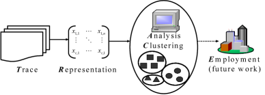
Figure 1: Illustration of the TRACE approach.

We use Fig. 1 to illustrate the conceptual flow of our approach in the paper, which we refer to as the TRACE approach. The five major components in the approach are: Trace, Representation, Analysis, Clustering, and Employment (or application). The work starts with the WLAN traces that capture realistic user behavior. We then focus on a specific representation distilled from the traces that captures important aspects of user behavior, as we introduce in section II. We conduct analysis and clustering upon the users based on the chosen representation, normalized association vectors, from section III to section VI. We first show the need for a good distance metric for clustering in section III. To achieve that goal, we conduct further analysis to understand the nature of user association patterns, and evaluate and contrast various summaries to capture its major trend in section IV. We then utilize a feature-based approach to achieve meaningful user clustering in section V and discuss its interpretation in section VI. Finally, we show-case one direct application, mobility-profile-based casting, of our user grouping in section VII, and briefly discuss other potential employment of the methods and findings in the paper in section VIII. Related work is discussed in section IX. The paper concludes in section X.

II Preliminaries

We first introduce the traces we analyze in the paper and the normalized association vector representation we choose. We also briefly introduce the necessary background knowledge about clustering in the section.

II-A Choice of Data Set and Representations

The widespread deployments of large-scale wireless LANs on university campuses have attracted high adoption from its community. These deployments have outgrown experimental networks and become a commodities. Due to its high penetration and diversity in users (as compared to corporate WLANs), campus networks are good platforms to study the behavioral pattern of WLAN users. To our benefit, great efforts have already been made to collect the user traces from several large WLAN deployments [11, 12]. We elect two WLAN traces collected from large populations for long durations for the study. The details for the selected traces are listed in Table I.

TABLE I: Facts about studied traces

Trace source	USC [13]	Dartmouth [14]
Time/duration	2006 spring	2004 spring
of trace	semester	quarter
	(94 days)	(61 days)
Start/End	01/25/06-	04/05/04-
time	04/28/06	06/04/04
Location	Building	Access point
granularity
Unique	137 buildings	545 APs/
locations		162 buildings
Unique MACs analyzed	5,000	6,582

While university WLAN traces are suitable for the study of user behavior, there are also shortcomings in these traces. The most important ones are (1) Users are not always online and many of them access the network sporadically. (2) Most WLAN users access the network with laptops, which are not always easily portable and limit the mobility of users while accessing the network. However, these WLAN traces are by far the most extensive publicly available traces and we can indeed discover interesting patterns. Note that our methods are not limited to the specific data sets we choose, and it would be of great interest to study traces from other mobile devices (e.g., cellphones, iPods), if available for a large population.

To understand user behavior from wireless network traces, the first fundamental task is to choose a representation of the raw data. We choose the patterns of users visiting various locations in the WLAN for the analysis. Visiting pattern is important to WLANs as mobility is one of its defining characteristics. When a WLAN user moves within the campus and associates with access points (APs) across the network, the set of APs with which the user associates is considered an indicator of the user’s physical location. From a social context, the places a person visits regularly and repeatedly usually have a stronger connection to her identity and affiliation. It is perhaps one of the important distinguishing factors for people with different social attributes.

We represent a user’s visiting pattern by what we refer to as normalized association vectors. The association vector is a summary of a user’s association with various locations during a given time slot. We choose to use a day as the time slot since it represents the most natural behavior cycle in our lives. The association vector for each time slot is an $n$-entry vector, $(x_{1},x_{2},...,x_{n})$, where $n$ is the number of unique locations (i.e., buildings) in the given trace. Note that, although WLAN traces provide better location granularity (at per-access point level), in this work we aggregate APs in the same building as a single location for better interpretation of user behavior. Each entry in the vector, $x_{i}$, represents the fraction of online time the user spends at the location during the time slot, i.e. we normalize the user association time with respect to his online time. With this representation, the conclusions we draw are not influenced by the absolute value of online time, which varies across a wide range among different users and different time slots of a given user. Note that the sum of the entries in the association vector, $\sum_{i=1}^{n}x_{i}$, is always $1$ if the user has been online during the time slot. We use a zero vector to represent the association vector when the user is completely offline for the time slot. To represent a user’s association preference for the long run, we construct the association matrix $X$ for the user, as illustrated in Fig. 2, i.e. we concatenate the association vectors for each time slot (day). If there are $n$ distinct locations and the trace period consists $t$ time slots, the association matrix for a user is a $t$-by-$n$ matrix.

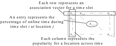
Figure 2: Illustration of association matrix representation.

Note that there are potentially many ways to represent user behavior from a rich data set. Different representations certainly provide different insights. Due to space limitations, we focus on the normalized representation for daily association vectors to illustrate our analysis, and briefly discuss about other alternatives in section Appendix A. Alternative Methods.

II-B Preliminaries of Clustering Techniques

Clustering (one of the key methods in unsupervised learning) is a widely-applied technique to discover patterns from data sets with unknown characteristics. It can be roughly classified into hierarchical or partitional schemes [1]. In this paper we use the hierarchical clustering, in which each element is initially considered as a cluster containing one member. Then, at each step, based on the distances between the clusters, two clusters that are the closest to each other among all cluster pairs are merged into one cluster with larger membership. This process continues until a clustering threshold has been reached, when all the inter-cluster distances for the remaining clusters are larger than a given distance threshold, or the remaining cluster number reaches a given target.

One major issue in applying clustering to a data set with unknown characteristics is that it is hard to pre-select a proper clustering threshold in advance. The indication of a good clustering result is that the distances between elements in the same cluster are low, and the distances between elements in different clusters are high. (i.e., there is a clear separation between inter-cluster and intra-cluster distance distributions.) Usually the clustering threshold comes from the domain knowledge or trial-and-error. Often the decisive factor for the quality of the clustering results is the selection of the distance metric, which is our main contributions.

III Challenges

As mentioned previously, the most important step in clustering is to define the similarity or distance metric between users. We highlight the challenges in selecting a proper distance metric with an example in this section.

An intuitive distance function between user association patterns of two individuals is to consider all the association vector pairs. Formally, we define the average minimum vector distance (AMVD) between users $A$ and $B$, $AMVD(A,B)$, as

$$AMVD(A,B)=\frac{1}{|A|}\sum_{\forall A_{i}\in A}{\mathbf{\arg}\>\;\min_{\forall B_{j}\in B}}d(A_{i},B_{j}),$$ (1)

where $A_{i}$ and $B_{j}$ denote an association vector of user $A$ and $B$, respectively. $|A|$ denotes the cardinality of set $A$. $d(A_{i},B_{j})$ denotes the Manhattan distance, defined as

$$d(a,b)=\sum_{i=1}^{n}|a_{i}-b_{i}|,$$ (2)

where $a_{i}$ and $b_{i}$ are the $i$-th element in vector $a$ and $b$, respectively. $AMVD(A,B)$ is the average of distances from each of the vectors in set $A$ to the closest vector (or the nearest neighbor) in set $B$. We define the $AMVD$ following the intuition that if every association vector in set $A$ is close to some association vector in set $B$, these sets should be similar. Note that, with this definition, $AMVD(A,B)$ is not necessarily equal to $AMVD(B,A)$. We define a symmetric distance metric between users $A$ and $B$ as $D(A,B)=(AMVD(A,B)+AMVD(B,A))/2$.

We apply the hierarchical clustering algorithm to users with the distance metric derived from AMVD. As mentioned earlier, a clustering algorithm requires properly chosen thresholds, and the particular choice is data-dependent. We experiment with various thresholds, and discover that for the USC trace, we can group the populations into $200$ clusters with a clear separation between inter and intra cluster distance distributions (Fig. 3 (a)), which is a qualitative indicator for a right clustering. However, the distance metric works poorly for the Dartmouth trace, as shown in Fig. 3 (b). The separation between inter and intra cluster distance distributions is not clear, regardless of cluster thresholds.

One problem with the $AMVD$ metric is that it considers all association vectors, i.e. it includes not only the important trends, but also the noise vectors when the users deviate from the dominant trend, leading to bad clustering results. A meaningful distance metric should capture the major trends of user behavior and be robust to noise and outliers. Another problem the $AMVD$ metric is its computation complexity. We have to calculate the distances between all $t^{2}$ pairs of association vectors for each user pair. If there are $N$ users the computation requirement is of order $O(N^{2}t^{2})$. Furthermore, it requires significant space to store $t$ association vectors for all $N$ users. Thus we would like to design a metric that is both (1) robust to noise and (2) computation and storage efficient. In order to achieve both goals, we start by studying the characteristics of the association patterns of a single user to validate the repetitive patterns or modes of behavior. We show that this study leads us to the appropriate distance metric.

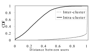
(a) USC.

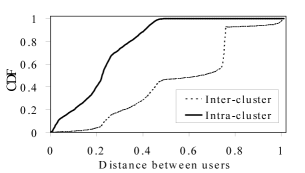
(b) Dartmouth

Figure 3: Cumulative distribution function of distances for inter-cluster and intra-cluster user pairs (AMVD distance).

IV Summarizing the Association Patterns

In this section, we identify association trends of an individual and construct a compact representation of her association matrices, which is suitable for distance computations used in clustering.

IV-A Characteristics of Association Patterns

We first understand the repetitive trend in a single user’s associations pattern, and how dominant the trend is (i.e., are there dominant behavioral modes?). We obtain this upon clustering the association vectors of a single individual.

Consider the clustering of the association vectors, $X_{i}$ for $i=1,...,t$ (i.e., row vectors of an association matrix $X$) of a single user. The identified clusters represent distinct behavioral modes of the user. Similar association vectors will be merged into a cluster in the process and the cluster size indicates its dominance - large clusters imply that the user follows consistent association patterns on many different days as its major behavioral modes.

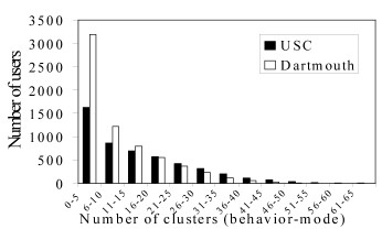
(a) Clustering threshold = 0.2

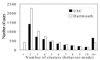
(b) Clustering threshold = 0.9

Figure 4: Distribution of number of clusters (behavioral modes) for users.

We apply clustering to the association vectors of each user in the USC and the Dartmouth traces using various clustering thresholds. The distribution of number of clusters (or behavioral modes) obtained are shown in Fig. 4. In Fig. 4(a), we use a small clustering threshold ($0.2$), with which only very similar association vectors are merged. We see that for the USC and the Dartmouth traces, respectively, about $50\%$ and $67\%$ of users have less than $10$ different clusters or behavioral modes (much fewer than total number of time slots, $94$ and $61$) with this low clustering threshold. This indicates the users have distinct repetitive trends in its association vectors. On the other hand, if we consider a moderate clustering threshold ($0.9$), we see in Fig. 4 (b) that users still show multiple behavioral modes. On average, with $0.9$ as the clustering threshold, the number of behavioral modes for USC and Dartmouth users are $5.57$ and $4.32$, respectively, and the users with the most behavioral modes have $32$ clusters in both cases.

Most of those users with two behavioral modes have a consistent association pattern: One mode corresponds to the association vectors when the user is offline, and the other one corresponds to the association vectors when the user is online. These users switch between online and offline behaviors from day to day, and when they are online, the association vectors are consistent and fall in a single behavioral mode. We refer to these users as single-modal users. On the other hand, we also observe many multi-modal users. These users show a more complex behavior: their association vectors form more than two clusters, which indicate that they display distinct behavioral modes when they are online. $71.9\%$ of users in USC and $59.4\%$ of users in Dartmouth are classified as multi-modal when the clustering threshold is $0.9$. Hence, we conclude that although users in WLANs are not extremely mobile, they do move and display various association patterns over a period of time.

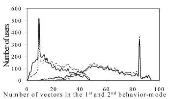
Figure 5: Distribution of association vectors in the first and the second behavioral modes for the USC trace. Right: the first cluster, Left: the second cluster.

To examine the degree of dominance of the most important behavior modes of users, we compare the most important behavioral mode and the second most important one in terms of their sizes. In Fig. 5 we plot the size (i.e. number of vectors) distributions of the first and the second behavioral modes under clustering threshold $0.2$ (solid lines) and $0.9$ (dotted lines) for USC users. We see that there is a clear separation between the sizes of these two behavioral modes. (i.e., the most dominant behavioral mode is much more important than the second most important one for most users.) Different clustering thresholds do not change the results much. In other words, observations of the most dominant behavioral mode could reveal user characteristic to a good extent for many users. Similar observations also hold for Dartmouth users.

We show the distribution of the size ratio between the largest and the second largest cluster in Fig. 6. Here we see for USC and Dartmouth, respectively, $36\%$ and $31\%$ of users have the two most important behavior modes with comparable sizes (i.e., with size ratio smaller than $2.0$ - The second most important behavioral mode is followed at least one half as often as the most important behavioral mode). Hence looking at the most dominant cluster exclusively could still be sometimes misleading and we might be ignoring information about the user’s detailed behavior. It is therefore desirable to have a summary that takes not only the dominant behavioral mode, but also the subsequent ones into account.

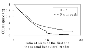
Figure 6: Complementary CDF for the ratio of the first behavioral mode size to the second behavioral mode size. Note that the X-axis is in log scale to make the graph more visible.

IV-B Summarization Methods

Now we investigate various ways to summarize the association vectors, and then judge their quality based on a specific metric - the significance score.

Average of association vectors

This is the simplest way to calculate a summary. Averaging naturally emphasizes the dominant behavioral mode (as there are more vectors in this mode). As users are not always online, the average should include only the online days and ignore the zero vectors, defined as

$X_{onavg}$, denoted as

$$X_{onavg}=\frac{\sum_{i=1}^{t}X_{i}}{\sum_{i=1}^{t}{\parallel X_{i}\parallel}_{1}},$$ (3)

where ${\parallel X_{i}\parallel}_{1}$ is the L1 norm of vector $X_{i}$ (recall that for online days, the elements in association vectors sum to 1).

Centroid of the first cluster

We observe for many users, the first behavioral mode is dominant. Hence we can use the centroid of vectors in the first non-trivial behavioral mode (i.e., if the first behavioral mode is the cluster of zero vectors, we take the second behavioral mode instead) as a summary. Formally,

$$X_{centroid1}=\frac{\sum_{X_{i}\in C_{1}}X_{i}}{\sum_{i=1}^{t}I(X_{i}\in C_{1})},$$ (4)

where $C_{1}$ denotes the largest non-trivial behavioral mode for the user and $I(\cdot)$ is the indicator function. Intuitively, it works well if the first behavioral mode is dominant, but less so if there are multiple behavioral modes with comparable importance for the user. We experiment with two different thresholds, $0.5$ or $0.9$, to identify the dominant behavioral mode.

In order to quantitatively compare the quality of the summary techniques, we propose to measure the significance score of a summary vector with respect to a user by summing the projections of all association vectors on the summary vector, normalized by the online days of the user.

$$SIG(Y)=\frac{\sum_{i=1}^{t}|X_{i}\cdot Y|}{\sum_{i=1}^{t}{\parallel X_{i}\parallel}_{1}},$$ (5)

where $Y$ is any summary vector. The physical interpretation of the significance score is the percentage of power in the association vectors $X_{i}$’s explained by the summary vector $Y$. Following the definition, we calculate the average score of the significance for $X_{onavg}$ and $X_{centroid1}$, and list them in Table II. We observe that the centroid of the first cluster better explains the behavioral pattern of a given user than the average, since averaging sometimes lead to a vector that falls between the behavioral modes.

TABLE II: The average significance score for various summaries of user association vectors

	$X_{onavg}$	$X_{centroid1}$	$X_{centroid1}$	SVD
		threshold 0.5	threshold 0.9
USC	0.646	0.716	0.702	0.764
Dartmouth	0.690	0.757	0.747	0.789

Singular Value Decomposition

We revisit our definition of the significance score in Eq. (5), and pose it as an optimization question: Given the association vectors $X_{i}$’s, what is the best possible summary vector $Y$ to maximize its significance? Mathematically, we want the vector $Y$ to be

$$Y=\arg\max_{\|v\|=1}\sum_{i=1}^{t}|X_{i}\cdot v|.$$ (6)

This is exactly the procedure to obtain the first singular vector if we perform singular value decomposition (SVD) [3] of the association matrix $X$. In other words, if we want the summary vector $Y$ to capture the maximum possible power in the association vector $X_{i}$’s, the optimal solution is to apply singular value decomposition to extract the first singular vector. We apply this technique and calculate the significance score in the last column in Table II. SVD provides the best summary. Hence we use the SVD-based summary, and defer the discussion of other summary techniques to section Appendix A. Alternative Methods.

IV-C Interpreting Singular Value Decomposition

In this subsection we explain other important properties of SVD as applied to the association matrices.

From linear algebra [3], we know that for any $t$-by-$n$ matrix $X$, it is possible to perform singular value decomposition, such that

$$X=U\cdot\Sigma\cdot V^{T},$$ (7)

where $U$ is a $t$-by-$t$ matrix, $\Sigma$ is a $t$-by-$n$ matrix with $r$ non-zero entries on its main diagonal, and $V^{T}$ is an $n$-by-$n$ matrix where the superscript ^T in $V^{T}$ indicates the transpose operation to matrix $V$. $r$ is the rank of the original association matrix $X$. The column vectors of the matrix $V$ are the eigenvectors of the covariance matrix $X^{T}X$, and $\Sigma$ is a diagonal matrix with the corresponding singular values to these eigenvectors on its diagonal, denoted as $\sigma_{1}$, $\sigma_{2}$, …, $\sigma_{r}$. These singular values are ordered by their values (i.e. $\sigma_{1}\geq\sigma_{2}\geq...\geq\sigma_{r}$). We can re-write Eq. (7) in a different form:

$$\tilde{X}_{k}=\sum^{k}_{i=1}u_{i}\sigma_{i}v_{i}^{T}.$$ (8)

Here $u_{i}$’s and $v_{i}$’s are the column vectors of matrix $U$ and $V$. They are used as the building blocks to reconstruct the original matrix $X$. With this format, SVD can be viewed as a way to decompose a matrix: It breaks the matrix $X$ into column vectors $u_{i}$, $v_{i}$ and real numbers $\sigma_{i}$. If we retain all these components (i.e., $k=rank(X)$), SVD is a lossless operation and the matrix $X$ can be reconstructed accurately. However, in practical application, SVD can be treated as a lossy compression and only the important components are retained to give a rank-$k$ approximation of matrix $X$. The percentage of power in the original matrix $X$ captured in the rank-$k$ reconstruction in Eq. (8) can be calculated by

$$\frac{\sum^{k}_{i=1}\sigma_{i}^{2}}{\sum^{Rank(X)}_{i=1}\sigma_{i}^{2}}.$$ (9)

For our data sets, users have much fewer behavioral modes than the number of association vectors, and for most users the dominant behavioral modes are much stronger than the others (c.f. Fig. 5). Hence we expect SVD to achieve great data reduction on the association matrices. This is indeed the case, as we show in Fig. 7: Most of the users have a high percentage of power in association matrix $X$ explained by a relatively low-rank reconstruction - For example, in the USC trace (Fig. 7(a)), if we use a rank-$1$ reconstruction matrix, it captures $50\%$ or more of power in the association matrices for more than $98\%$ of users, and a rank-$3$ reconstruction is sufficient to capture more than $50\%$ of power in association matrices for all users. Even if we consider an extreme requirement, capturing $90\%$ of power, it is achievable for $68\%$ of users using a rank-$1$ reconstruction matrix, and for more than $99\%$ of users using at most a rank-$7$ reconstruction matrix. Similar observations can be made for Dartmouth users (in Fig. 7(b)). For both campuses, five components are sufficient to capture $90\%$ or more power for most (i.e., more than $90\%$) of the users. This indicates although users show multi-modal association pattern, for most users the top behavioral modes are relatively much more important then the remaining ones.

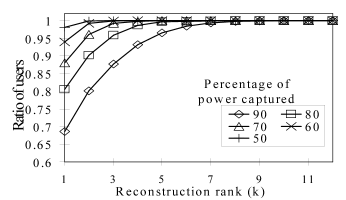
(a)USC.

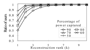
(b)Dartmouth.

Figure 7: Low association matrices dimensionality: A high target percentage of power is captured with low rank reconstruction matrix for many users.

If a low-rank reconstruction of the association matrix is achievable, it is natural to ask for the representative vectors for the behavioral modes of a user. For this purpose, SVD can be viewed as a procedure to obtain representative vectors that capture the most remaining power in the matrix. Mathematically,

$$\begin{split}u_{1}&=\arg\max_{\|u\|=1}\|X\cdot u\|\\ u_{k}&=\arg\max_{\|u\|=1}\|(X-\sum^{k-1}_{i=1}Xu_{i}u_{i}^{\prime})u\|\;\;\;\forall k\geq 2.\end{split}$$ (10)

We can interpret the singular vectors, $u_{j}$’s, as the vectors that describe the user’s behavioral modes in decreasing order of importance in the association matrix $X$, with its relative weight (or the importance) quantified by $\sigma_{j}^{2}/\sum^{r}_{i=1}\sigma_{i}^{2}$, following Eq. (9). In the paper we refer to these vectors as eigen-behavior vectors for the user.

The eigen-behavior vectors, $u_{j}$’s, are unit-length vectors. The absolute values of entries in an eigen-behavior vector quantify the relative importance of the locations in the user’s $j$-th behavioral mode. For example, suppose a given user visit location $l$ almost exclusively, then in his first eigen-behavior vector, the entry corresponds to location $l$ would carry a high value (i.e. close to $1$), and the weight of the first eigen-behavior vector, $\sigma_{1}^{2}/\sum^{r}_{i=1}\sigma_{i}^{2}$, shall be high. With a set of eigen-behavior vectors and their corresponding weights, we can capture and quantify the relative importance of a user’s behavioral modes.

There are several benefits of applying SVD to obtain the summary as compared to other schemes: (1) SVD provides the optimal summary that captures the most remaining power in the original matrix with each additional component. (2) The components can be used to reconstruct the original matrix, while the calculation of average or centroid vectors are non-reversible. Thus SVD provides a way to compress user association vectors and helps us save storage space. (3) Not only the most important behavioral mode, but also the subsequent ones can be systematically obtained with SVD, with a quantitative notion of their relative importance.

V Clustering Users by Eigen-behavior vectors

In this section, we first define our novel distance measure based on the eigen-behavior vectors and then use it for clustering.

V-A Eigen-behavior Distance

Suppose $u_{i}$’s and $v_{j}$’s are the eigen-behavior vectors of two users, $i=1,...,r_{u}$ and $j=1,...,r_{v}$ where $r_{u}$ and $r_{v}$ are the ranks of the corresponding association matrices. The similarity between the two users can be calculated by the sum of pair-wise inner products of their eigen-behavior vectors $u_{i}$’s and $v_{j}$’s, weighted by $w_{u_{i}}$ and $w_{v_{j}}$. Our measure of similarity between two sets of eigen-behavior vectors, $U=\{u_{1},...,u_{r_{u}}\}$ and $V=\{v_{1},...,v_{r_{v}}\}$, is defined as:

$$Sim(U,V)=\sum^{r_{u}}_{i=1}\sum^{r_{v}}_{j=1}w_{u_{i}}w_{v_{j}}|u_{i}\cdot v_{j}|.$$ (11)

Higher similarity index $Sim(U,V)$ indicates that the eigen-behavior vectors $U$ and $V$ are more similar, and hence the corresponding users have similar association patterns. We define the eigen-behavior distance between users $U$ and $V$ as $D^{\prime}(U,V)=1-(Sim(U,V)+Sim(V,U))/2$.

Using the eigen-behavior distance also reduces the computation overhead. If we use only the top-$5$ components (which captures more than $90\%$ power as in Fig. 7), instead of going through $t$-by-$t$ pairs of original association vectors as in section III, we reduce the distance calculation to $5$-by-$5$ pairs. Since we have at least $61$ days in the traces, this is at least a $(61/5)^{2}\approx 148$ fold saving for all $N^{2}$ pair of users. By paying the pre-processing (i.e., SVD for all $N$ users) overhead of $O(Nt^{2})$, we can reduce the distance calculation complexity from $O(N^{2}t^{2})$ to $O(c\cdot N^{2})$. Since users follow repetitive trends in the association patterns, its total eigen-behavior vectors would not grow with the number of time slots, $t$. If we consider longer traces or association vector representations in finer time scale, the reduction can be even more significant. In the following computations, we consider only the eigen-behavior vectors that capture at least $0.1\%$ of total power.

V-B Significance of the Clusters

We cluster users based on eigen-behavior distance and again validate the results by plotting the intra-cluster and inter-cluster distance distributions, when we consider $200$ clusters. With the eigen-behavior distance, for both USC and Dartmouth traces, there is a better separation between the CDF curves (Fig. 8) as compared to the results with the AMVD distance (Fig 3), indicating a meaningful clustering. This proves the eigen-behavior distance is a better metric than the AMVD distance as it helps us to group users into well-separated behavioral groups based on their WLAN association preferences, for both campuses.

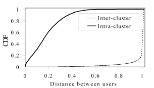
(a) USC.

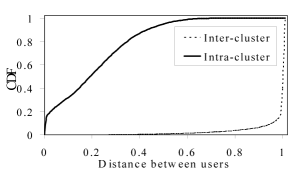
(b) Dartmouth.

Figure 8: Cumulative distribution function of distances for inter-cluster and intra-cluster user pairs (eigen-vector distance).

We further validate whether the resulting clusters indeed capture users with similar behavioral trends. We compose the joint association matrix by concatenating the daily association vectors of a cluster of $m$ similar users in a larger $mt$-by-$n$ matrix, where $n$ is the number of locations and $t$ is the number of time slots. When we perform SVD to the joint association matrix, the top eigen-behavior vectors represent the dominant behavioral patterns within the group. If the users in the group follow a coherent behavioral trend, the percentage of power captured by the top eigen-behavior vectors should be high. On the other hand, if association vectors of users with different association trends are put in one joint association matrix, the percentage of power captured by its top eigen-behavior vectors should be much lower. Among all clusters, we pick those with more than five users, and compare the cumulative power captured by the top four eigen-behavior vectors of these clusters with random clusters of the same size in scatter graphs, Fig. 9. Clearly, most the dots are well above the $45$-degree line for both campuses. This indicates the users in the same cluster follow a much stronger coherent behavioral trend than randomly picked users, pointing to the significance of our clustering results.

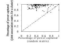
(a) USC(129 clusters)

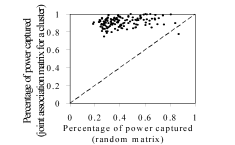
(b) Dartmouth(136 clusters)

Figure 9: Scatter graph: Cumulative power captured in top four eigen-behavior vectors of random matrices (X) and joint association matrices formed by users in the same cluster (Y). Only clusters with $5$ or more members are included.

We would also like to see if each cluster from the population shows a distinct behavioral pattern. To quantify this, we obtain the first eigen-behavior vector from each group and calculate its significance score, defined in Eq. (5), for all the groups. The results confirm with our goal of identifying groups following different behavioral trend: For the USC trace, the first eigen-behavior vectors obtained from the joint association matrices have an average significance score of $0.779$ for their own clusters and an average score of $0.005$ for other clusters, indicating the dominant behavioral trends from each cluster is distinct. The corresponding numbers for the Dartmouth trace are $0.727$ and $0.004$, respectively.

We conclude that we have designed a distance metric that effectively partitions users into groups based on behavioral patterns. In addition, these clusters are unique with respect to behavioral trends.

VI Interpretation of the Clustering Results

In this section we analyze and interpret the results of clustering for both university campuses from social perspective.

First we analyze the group size distribution, as shown in Fig. 10. We observe the distributions of group sizes are highly-skewed for both campuses. There are dominant behavioral groups that many users follow: the largest groups in the campuses include $504$ and $546$ members, out of the population of $5000$ for USC and $6582$ for Dartmouth, respectively. The ten largest groups combined account for $39\%$ and $33\%$ of the total population, respectively. On the other hand, there are also many small groups, or even singletons, for both populations: out of the $200$ clusters, there are $68$ and $57$ of them with less than five members, respectively, and in both campuses about half of the groups have less than $10$ members. More interestingly, we observe that besides these small clusters, the distribution of the cluster size follows a power-law distribution. In Fig. 10, we plot the straight lines that illustrate the best power-law fits. The slopes for these lines are $-0.67$ for Dartmouth and $-0.75$ for USC, respectively. The power law distribution of group sizes may be related to the skewed popularity of locations on campuses - it has been shown that the number of patrons to various locations differ significantly[8]. However, the link between the distributions of number of patrons and the distribution of group sizes is not direct. While the most-visited locations on both campuses easily attract thousands of patrons, these people are broken into different behavioral groups depending on their association preferences.

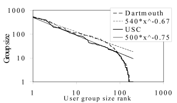
Figure 10: Rank plot (group size ranking v.s. group size) in log-log scale. User group size follows a power-law distribution.

We now study the detailed behaviors of each cluster by using the eigen-behavior vectors and their relative weights to understand the detailed preferences of the groups. We discover for most of the groups, their top eigen-behavior vectors dominate i.e. the contribution of the second-most important location is almost invisible in the first eigen-behavior vector. Similar relationship holds between the second-most important location and the third-most important one, and so on. Hence the association behavior of the group can be described by a sequence of locations of decreasing importance with a clear ordering. This observation matches with the current status of WLAN usage: people tend to access WLAN at only a limited number of locations, and the preference of visiting locations is skewed [16]. For such users, its most visited locations might be sufficient to classify them.

Most large user clusters belong to the fore-mentioned case. The largest clusters on both campuses include the library visitors, as expected, since libraries are still the most visited area on university campuses. For the USC campus, the largest user cluster visits the library (the first eigen-behavior vector has a single high-value entry corresponding to the library, and this eigen-behavior vector captures $83\%$ of the power in the joint association matrix for the group), followed by a couple locations around the Law school ($4.45\%$) and the school of Communication ($4.5\%$), both are popular locations on campus. For the Dartmouth campus, the largest user cluster visits LibBldg2 ($72.85\%$), followed by LibBldg1 ($5.13\%$), SocBldg1 ($3.56\%$), and LibBldg3 ($1.93\%$). It seems this group consists of library patrons who mainly move about the public area on the campus and access the WLAN from these locations.

While libraries are popular WLAN hot spots, we also discover many user clusters that rarely visit these locations. The second largest cluster for USC consists of users visiting mostly the Law school ($89.73\%$ of power), school of accounting ($6.37\%$), and a couple of locations close to the Law school ($0.59\%$). For Dartmouth, the second largest cluster visits AcadBldg18 ($56.38\%$), AcadBldg6 ($13.4\%$), ResBldg83 ($10.15\%$), AcadBldg31 ($3.5\%$), AcadBldg7 ($3.12\%$), which seems to be a group of students going to classes at multiple academic buildings. We have also observed various clusters featured different dorms and classrooms as their most visited location from both campuses.

On the other hand, we have also discovered groups with multiple high-value entries in its top eigen-behavior vectors from both campuses. One prominent example from USC trace consists of $32$ users, who visit buildings VKC and THH, two major classrooms on the USC campus. The top two eigen-behavior vectors of the cluster both consist of two high-value entries corresponding to these two buildings, and they capture $63.14\%$ of power in the joint association matrix. This cluster consists of users who visit these two locations with similar tendency, according to the eigen-behavior vectors, and such distinct behavioral trend exists for $32$ users in the population. This cluster is a good example to show why it is not sufficient to merely use the most dominant behavioral mode (or the most-visited location) of a user to classify it. If the centroid of the dominant behavioral mode (i.e., Eq (4)) is used to classify users, the behavioral trend of visiting multiple locations with similar tendency will not be revealed. Instead, among the $32$ users, $13$ are classified with others who visit VKC frequently, $10$ are classified with those who visit THH frequently, and the rest are put into various groups. As portable wireless devices gain popularity, we expect to see more users displaying diverse behavioral trends in terms of network usage. To fully capture such behavior, averaging-based summary is not sufficient, and this is where SVD shows its strength the most.

Interestingly, we also discover many small clusters with unique behavioral patterns that deviate from the ”main stream” users in both traces. For example, in the USC trace, there is a small cluster of eight users who visit exclusively a fraternity house. Probably these are the people who live there. In the Dartmouth trace, there is a cluster of eight users who visit mostly athletic buildings (AthBldg5 ($90.9\%$), AthBldg10 ($4.62\%$), AthBldg2 ($3.14\%$), AthBldg3 ($0.8\%$), and ResBldg26 ($0.54\%$)). These are probably either athletes or management staffs of the athlete facility. Such findings substantiate our motivation of the study: as the wireless technology prevails, we can expect users to display diverse behavioral patterns that reflect to their personal preferences, and it is important to capture such behavioral trend and quantify its significance.

To sum up, we have demonstrated a systematic way to identify distinct behavioral groups within on-campus populations, by using clustering based on association features obtained from large-scale wireless network traces. The method and findings are useful for various applications, as we show in the subsequent section with a case study of profile-based casting, and discuss other potential applications in the next section.

VII Case Study: Mobility-profile-based Casting Protocol

VII-A Preliminaries

Delay tolerant networks (DTNs)[22] are networks characterized by sparse, time-varying connectivity, in which end-to-end spatial paths from source to destination nodes are often not available. Messages are stored in intermediate nodes and moved across the network with nodal mobility. One particular important decision to make for nodes in DTN is whether to forward a packet to other nodes they encounter (i.e., move into the radio range) with. Such decisions have implications on many aspects of how efficiently the routing strategies work, such as delay, overhead, and message delivery rate.

VII-B A Mobility PROFILE-CASTing Protocol

In the paper we consider the scenario where the message sender is interested in forwarding messages to users with a similar mobility profile. For example, a student loses a wallet and wishes to send an announcement to other fellow students who visit similar places often as he does to look for it. Or, for location specific announcements such as power shutdown in parts of campus directed only to patrons of the specific area. Note that this application is different from geo-casting, which targets at the nodes currently within a geographical region as the receivers. Our target receivers are nodes with a certain mobility profile, regardless of their actual locations at the time the message is sent. To enable such profile-based casting services, it is important to have a descriptive representation for user behavioral profiles and a measure of the similarity between users, to guide the message forwarding decisions.

In previous sections, we analyze two large scale WLAN user association traces[13, 14] and represent user mobility in the form of daily association vector to classify the whole user population into distinct behavioral groups with unsupervised learning techniques. In this section, we take these behavioral groups as the targets for mobility profile-based casting.

The details of our similarity-based profile-based casting is as follows: Users in the network are not aware of the centralized decision of user grouping based on similarity in their mobility. Instead, when two users meet each other, they exchange the mobility profiles (i.e., vectors with their relative importance (weights)) of their previous behavioral patterns and decide whether they are similar at the spot, according to Eq. (11). If the similarity index is larger than a threshold, they exchange the message. Note this decision is solely local, involving only the two encountered nodes. The philosophy behind the protocol is, if each node delivers the message only to others with high similarity in mobility profile, the propagation of the message copies will be scoped.

VII-C Evaluation and Comparison

We compare the performances of following schemes with the similarity-based protocol : (1) Flooding: The nodes in the network are all oblivious to user mobility profiles and blindly send out copies of the message to nodes who have not received it yet. This scheme is also known as epidemic routing [24]. (2) Centralized: In this ideal scenario, all nodes acquire the centralized knowledge of the behavioral group membership, and only propagate the message to others if they are in the same group. The message will never propagates to an unintended receiver. (3)Random-transmission (RTx): The current message holder sends the message to another node randomly with probability $p$ when they encounter, and never transmits again (i.e., only the node who last received the message will transmit in the future). Loops are avoided by not sending to the nodes who have seen the same message before. This process continues until a pre-set hop limit is reached.

We utilize the USC trace [13] to study the message transmission schemes discussed above empirically. We use the trace for user mobility and assume that two nodes are able to communicate when they are associated to the same access point. Note that the WLAN infrastructure is merely used to collect user location information, and the messages can be transferred only between the users without using the infrastructure, as in [23]. We split the WLAN trace into two halves. The first half of the trace is used to determine the grouping of users based on their mobility and we choose the number of clusters to be $200$. Then we evaluate the group-casting protocol performances using the second half of the same trace. For each group with more than $5$ members, we randomly pick $20\%$ of the members as the source nodes sending out a one-shot message to all other members in the same group.

The performance metrics used are as follows: (1) Delivery ratio: The number of nodes receiving the message over the number of intended receivers. (2) Delay: The average time taken for a scheme to deliver the messages to recipient nodes. (3) Overhead: The total number of transmissions involved in the process of message delivery.

We choose flooding (i.e., epidemic routing) as the baseline for our evaluation and show the relative performance of the other group-casting protocols relative to that of epidemic routing in Fig. 11. In the graph we see that flooding has the lowest delay and the highest delivery ratio as it utilizes all the available encounters to propagate the message. However, it also incurs significant overhead. The average delay, which is the lowest possible under the given encounter patterns, is in the order of days ($3.56$ days in this particular case). Group-casting based on centralized clustering information, the ideal scenario, shows great promise of behavior-aware protocols, as it significantly reduces the overhead while maintains almost perfect delivery ratio, with a little extra delay. However, it is not realistic to assume such centralized knowledge.

For the similarity-based protocol, its aggressiveness can be fine-tuned with the forwarding threshold of the similarity index. Experiment results show a significant reduction of overhead (only $2.5\%$ of flooding) at the cost of delivery ratio if we set a high threshold such as $0.7$ (i.e., sending almost exclusively within the same group). Setting a low threshold (e.g., $0.5$) leads to better delivery ratio ($92\%$ of flooding) but still cuts the overhead to $45\%$ of flooding. For the RTx protocol, although the overhead can be controlled with the hop-limit (which we set as $TTL$ times of the group size), we see that the delivery ratio is lower than that of the similarity-based protocol with comparable overhead (comparing similarity $0.6$ with RTx $TTL=9$, the former has $30\%$ higher delivery ratio than the later) because in many cases the message is transmitted to some node out of the desired group and there is no knowledge to direct its propagation. Further more, the average delay for the delivered messages is much longer than in the other protocols where multiple copies of message propagate in the network. In addition, we try the RTx protocol with various $p$ and $TTL$ values and find it is not as flexible as the similarity-based protocol in which the parameters can be tuned to trade overhead for better delivery ratio.

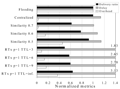
Figure 11: Relative performance metrics of the group-casting schemes normalized to the performance of flooding.

VIII Discussions

VIII-A Potential Applications

The insights of user grouping obtained from our analysis can be applied in many other ways. We discuss some of these application in this section, including (1) network management, (2) user modeling, (3) behavior-aware services.

Network Management Our analysis provides a different view of network management. WLAN management and planning could be done by monitoring the activities of individual APs in order to identify the busy ones. From the clustering technique, the manager can identify user groups and the relative importance of locations to each group. Such information can be helpful in terms of load prediction and planning. For example, if the business school is going to expand, by checking the behavioral groups of business school students, it is possible to predict its impact on the load of different parts of the WLAN. For better understanding, one may also observe the change in the group structure with time and across semesters.

The SVD techniques detailed in this paper also provides a succinct way to express the normal behavior of a given user. Once the norm of the user’s behavioral pattern is established, the system administrator could use the knowledge for behavioral abnormality detection. Obvious deviation in current behavior from the norm could be due to an impersonation attack or theft of the device, and should be brought to the administrator’s attention depending on the policy.

User Modeling Results from the clusters of users could help us to propose more realistic models for WLAN users, which is a challenge and a necessity for evaluating network protocols. Although mobility models with groups of user is not a new idea[25], there has been little work in realistic models based on groups. Our decomposition approach provides two pieces of important information: (1) the distribution of group sizes follows a power-law distribution and (2) the detailed eigen-behavior vectors of the groups. With such information, one can set up generative model with the group sizes and the weights for frequently visited locations (e.g., its communities[26]) properly to evaluate their impacts on the network.

Behavior-aware Services In future, we expect the wireless devices have to be very portable and personalized. Hence, the services provided could be highly personalized, or at least customized based on the interest groups. Our method would facilitate to identify the dominant groups. The case study in the previous section shows that we can utilize mobility profile as a basis for such grouping and guidance of message delivery. Certainly, different representations of users (e.g. hobbies, interests) that fit into the context might also be utilized rather, but our method would still be applicable. Furthermore, the service providers could assign a target behavioral vector to describe the property of target users, and the user devices could easily determine potential customers using a significance score (i.e., Eq. (5)) to compare its eigen-behavior vector to the target behavioral vector. We refer to this scenario as interest-based grouping and profile-casting, and it is our future work.

In addition to clustering, the eigen-behavior vectors could also provide an efficient mechanism for users to exchange their behavioral features in order to make new friends. Such social profiles could be applied in applications in social networking, such as behavior pattern oriented matching.

As large-scale city-wide WLAN deployments become commonplace, solutions to issues in management, service design, and protocol validation could immensely benefit from insight into the behavioral patterns of the users or the society. We believe that our framework will be able to provide a the behavioral patterns and help find solutions to several problems ranging from wireless network management to understanding basic social behavior of users armed with mobile devices in large WLANs.

VIII-B Alternative Representations and Metrics

We have evaluated our TRACE approach extensively with other distance metrics and representations of the data. Due space constraints, we only briefly discuss them here. Please refer to Appendix A for more details.

We design distance metrics with other types summaries in section IV-B, and they lead to user partitions similar to that from the SVD-based summary, since in current WLANs, most users have a dominant behavioral mode so simple summaries suffice to capture the trends. However, SVD is able to discover repetitive trends when users have a complicated pattern of visiting association points, while other methods cannot, as we argue in section VI.

We also consider several other representations. Without normalization (i.e., the entries in the association vectors represent the absolute duration of association), the most active users are classified similarly as in the case of normalized representation, but the less active users fall in different clusters due to their sporadic usage of WLAN. Our idea is to view a user’s behavior based on the fraction of time she spends at a location. We also explore the clustering by using both finer location granularity ( i.e., use each AP as a unique location) as well as finer time granularity (i.e. one association vector for each three-hour period). The resulted clusterings are similar to what we obtain, indicating the time-scale of daily vectors with per-building location granularity provide sufficient information.

On a different note, it may be of independent interest to use our representations in other domains in different type of networks. For example, in encounter-based networks [21], a representation of encounter probability or duration would be appropriate. We plan to investigate this in our future work.

IX Related Work

As wireless networks gain popularity, it is extremely important to understand its characteristics realistically. Along this line, there have been great efforts to collect traces from WLAN users. For examples, see [8, 16, 9, 10]. Many more traces have been made available through efforts to build libraries of measurement traces [12, 11].

Although user association pattern has been one major focus in studies about WLANs, for most previous works the focus is either on aggregated statistics or on association models for individual user. For the aggregate statistics, the current operating status of WLANs is studied extensively, including user association preferences and durations, mobility and hand-off, among others. Henderson et al. focuses on the comparison of the same campus during different time periods[8]. Balazinska et al. emphasizes on the mobility of corporate WLAN users[9]. [10] is a study specific to PDA users and their mobility. These traces are compared in [16] based on aggregate statistics. For most of the modeling works, the focus is to obtain particular statistics about users and to establish a model based on these quantities. In most of these modeling efforts, the users are considered as independent samples from a uniform population. In [20] the user association durations are modeled by BiPareto distributions. In [19] the authors match user session lengths and hand-off probabilities between APs to generate a mobility model. In [17, 18], the authors further cluster the locations (i.e., AP) based on the number of user hand-off between them to generate a hierarchy in user hand-off model. Hsu et al. explicitly models periodicity of users visiting their favorite locations[26]. There are hardly any studies on understanding the relationships between users in the literature. The only excpetion we are aware of is perhaps [5], where Kim et al. look into the range of movement of users, and classify users based on the periodicity of the movement range. We provide a further step towards this understanding by classifying users into groups of similar behavior. This provides a different and important perspective to understand user association patterns.

There are several papers in the literature that also use clustering techniques. One with a similar goal to ours is [5], which classifies users based on a different representation. In their paper, users are classified based on the dominant periods in their movement (e.g. those who display strong daily or weekly movement patterns) and their longest movement ranges, but not based the location preferences. Hence the results have different interpretations to ours. In [6] the authors apply clustering technique to the trace of location coordinates of a user to discover significant places for the user, but they have not focused on classifying users.

The technique we utilize to obtain association features from users, singular value decomposition[3], is widely-applied to discover linear trends in large data sets. It is closely related to principal component analysis [2]. In [7], the authors utilized PCA to decompose the traffic flow matrices for ISP networks and understand the major trends in the traffic. Our application of SVD to individual user association matrices is similar in spirit to their work. Note that it is typical for people to follow dominant routines in lives, hence we expect the SVD approach to be applicable to various human behavioral data sets. In [4], the authors also use PCA to discover trends in a cellphone user group, which is similar to our analysis on individual users. In this paper, in addition to analyzing much larger data sets, we further compare user similarity and define distance metrics to classify wireless network users into groups with robust validation. Note that in order to make the eigen-behavior vectors obtained from all users comparable, we need to keep the origin fixed among all association matrices. Hence we adopt a variant, called uncentered PCA [2] where the mean of each dimension is not subtracted. It has been used to study the diversity of species at various sites[15].

X Conclusion

In this paper, we classify groups of WLAN users based on the trends in their association patterns in two major university campuses by leveraging clustering techniques and our systematic TRACE approach. We design a novel distance metric between users based on the similarity of their eigen-behavior vectors, obtained through singular value decomposition (SVD) of the association matrices. SVD is the optimal way to capture underlying trends in the data set, and we have shown although many (at least $60\%$) users display multi-modal behavioral modes, SVD is able to capture at least $90\%$ of power in association matrices for most users with at most five components. This also leads to space and time efficient computations.

The eigen-behavior distance leads to a meaningful partition of users. We establish that WLAN users on university campuses form a diverse community, which includes hundreds of distinct behavioral groups in terms of association patterns. The size of the groups follows a power-law distribution on both campuses. While the large groups account for a major part of the population (the top ten groups account for at least $33\%$ of population in our data sets), there exist many small groups with unique association patterns. In spite of the very different location and demography of the two university campuses, it is surprising to find out the qualitative commonalities of the user behavior trends.

While distance metrics based on simple summaries (e.g., average or centroid of the dominant behavior mode) suffice for most current WLAN users, our study indicates that SVD is capable to capture user association trends in complex situations e.g. when users visit several distinct locations on different time slots (e.g. days). As personalized wireless devices become more popular, WLANs become ubiquitous and their powerful combination impacts our daily lives, a powerful tool to understand the user behavior is essential. Such understanding could lead to better network management, user behavior modeling, or even behavior-aware protocols and applications.

Appendix A. Alternative Methods

Besides the normalized association vectors and eigen-behavior distance obtained through SVD, there are many other potential representations of user association behavior and distance metrics. In this section we discuss about these alternatives and some results we obtain with those.

X-A Various Distance Metrics

We establish a meaningful partition of both user populations in Fig. 8 with the eigen-behavior distance. However, we have to note that the other summaries presented in section IV-B could also be used to obtain distance metrics. For these single-vector summaries, such as the average of association vectors ($X_{onavg}$, Eq. (3)) or centroid of the first cluster ($X_{centroid1}$, Eq. (4)), we define distance metrics between users by simply calculating the Manhattan distance (Eq. (2)) between the corresponding summary vectors. With these distance metrics, we could also arrive at meaningful partitions of user populations and hence those are valid metrics, too. We show two such examples in Fig. 12 - the general observation is that while $X_{onavg}$ leads to less well-separated clusters than the eigen-behavior distance, $X_{centroid1}$ leads to even better results.

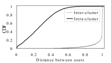
(a) USC, distance between average of association vectors.

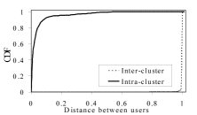
(b) Dartmouth, distance between centroid of the first behavioral mode.

Figure 12: Cumulative distribution function of distances for inter-cluster and intra-cluster user pairs (other distance metrics).

We need to further compare these different partitions of the user population to understand their properties. We choose to use the Jaccard index [27] to compare the similarity between different partitions of the same population. The Jaccard index between two partitions on the same population is defined as

$$J(P,Q)=r/(r+u+v),$$ (12)

where $r$ is the number of user pairs who are partitioned in the same cluster in both partition $P$ and $Q$ (i.e., where the two partitions agree on the classification). $u$ (or $v$) is the number of pairs who are in the same cluster in $P$ (or $Q$) but in different clusters in $Q$ (or $P$) (i.e., where the two partitions disagree). We choose the Jaccard index among many other indices for partition similarity due to its low variance on partitions with the same transfer distance [27]. For both traces, we list the Jaccard indices between user partitions from various distance metrics (Average and the Centroid of first behavioral mode) and the partition from the eigen-behavior distance in Table III. The Jaccard indices are mostly in the range of $0.7$ to $0.8$, indicating the partitions are in fact similar. The better separation between intra and inter cluster distance distributions with the $X_{centroid1}$ metric is partly because the distances are calculated based on a subset of association vectors with a coherent trend, discarding other vectors. Nonetheless, different distance metric has its own emphasis. While we argue in section VI with an example that eigen-behavior distance is useful for classifying users with multiple frequently visited locations with similar preferences, this is not always the only goal. Depending on the application, sometimes one may want to consider only the first behavioral mode and ignore the others.

TABLE III: Jaccard indices between user partitions based on eigen-behavior distances and various distance metrics.

Distance	Average	Centroid w/	Centroid w/
metric		threshold = 0.5	threshold = 0.9
USC	0.757	0.741	0.696
Dartmouth	0.801	0.706	0.710

Instead of applying SVD, one may propose to use the centroids for all behavioral modes of a user as a summary. However, the behavioral mode for each user is dependent on the clustering threshold, and it is not simple to choose one that works well for many users, considering the diversity. On the other hand, SVD does not require parameter tuning, and is optimal in the sense of capturing remaining power in the association matrix, so we choose it over the multiple centroids method, if all behavioral modes of a user should be considered.

X-B Various Data Representations

In this section we discuss about alternative representations of user behavior and compare the findings with the normalized association vector we choose in the paper.

In section II-A we propose to use normalized association vector in order to mitigate the differences of user activeness across users and across time slots for a given user. This is effective if the preference of the user for each time slot is the focus of study. For example, if a user visits exclusively location $A$ or $B$ on different days, for similar number of days, one way to understand the user behavior is that locations $A$ and $B$ are of the same importance for the given user, since he visits these two places exclusively with similar frequency. However, if the user stays at location $A$ whenever he visits for much longer duration than $B$, the normalized vector would not reveal such information. On the other hand, if absolute association time is used in the vectors, the large time spent at location $A$ will hide his visits to $B$ when SVD is applied to extract eigen-behaviors from the user (i.e., vectors with large association time to $A$ dominate the power of the matrix), albeit the user pays a lot of visits to $B$.

Both representations may be of interest to some applications. So instead of arguing the importance of one over the other, we try to understand its impact on how the users are clustered. Using the USC trace as an example, we compare the results of user partitions using absolute association time vectors and normalized association vectors. We observe that the most active users (i.e. The first quarter in terms of online time) are almost classified the same regardless which representation is used, with Jaccard index $0.9652$. This is the case since the most active users are almost always on, and the representation does not make much difference. We see the Jaccard indices drop to $0.7910$, $0.7090$, and $0.6096$ for the second, third, and fourth quarter of users in terms of activeness, respectively, a clear decreasing trend. The least active users are more sensitive to the choice of representation due to their sporadic usage of WLAN.

Time slot sizes to collect the association vectors is another dimension to experiment with. In addition to daily vectors, we consider two other schemes: (1) Generate association vectors for every three-hour time slot. We compare the partitions generated by this fine-grained representation with the partition generated by the daily representation, and get the Jaccard indices of $0.787$ and $0.778$ for USC and Dartmouth, respectively. This indicates that a finer time scale does not change the user classification much, and one day interval would be sufficient to capture important trends in user behavior. We also try (2) generate association vectors only during the time frame between 8AM to 4PM, the busy part of a day, and compare the subsequent partition with the partition generated by the daily representation in which the whole day is included. With this representation, the two traces give very different result - the Jaccard indices are $0.752$ and $0.033$, respectively. Hence it is not always sufficient to use only the behavior trends during working hours to classify users.

The choice of location granularity in the representation is important to understand the results. We have also try to use access points as locations for Dartmouth trace as the information is available. For most of the studies, the observations are similar to what we present in the paper, although one can expect to see more distinct behavior groups from the population if finer location granularity is used. However, it is not easy to interpret these groups meaningfully unless we have the information about detailed AP locations within the buildings and the significance of its covered area in social context. On the other hand, it is also possible that a group of buildings bear a higher-level meaning in social context (e.g., Several close-by dorms form a ”residential area”, or close-by buildings shared by the students from the same department), and it is also related to understand user visiting preferences from a higher-level behavioral context (e.g., home, at work, at class, etc.). We leave this as future work.

References

- [1] A. Jain, M. Murty, and P. Flynn, ”Data Clustering: A Review,” ACM Computing Surveys, vol. 31, no. 3, September, 1999.
- [2] I.T. Jolliffe, Principal Component Analysis, second ed., Springer series in statistics, published 2002.
- [3] R. Horn and C. Johnson, Matrix Analysis, Cambridge University Press, published 1990.
- [4] N. Eagle and A. Pentland, ”Reality mining: sensing complex social systems,” in Journal of Personal and Ubiquitous Computing, vol.10, no. 4, May 2006.
- [5] M. Kim and D. Kotz, ”Periodic properties of user mobility and access-point popularity,” Journal of Personal and Ubiquitous Computing, 11(6), August, 2007.
- [6] J. Kang, W. Welbourne, B. Stewart, and G. Borriello, ”Extracting places from traces of locations,” in SIGMOBILE Mobile Computing and Communication Review, vol. 9, no. 3, July 2005.
- [7] A. Lakhina, K. Papagiannaki, M. Crovella, C. Diot, E. D. Kolaczyk, and N. Taft, ”Structural Analysis of Network Traffic Flows,” ACM SIGMETRICS, New York, June 2004.
- [8] T. Henderson, D. Kotz and I. Abyzov, ”The Changing Usage of a Mature Campus-wide Wireless Network,” in Proceedings of ACM MobiCom 2004, September 2004.
- [9] M. Balazinska and P. Castro, ”Characterizing Mobility and Network Usage in a Corporate Wireless Local-Area Network,” In Proceedings of MobiSys 2003, May 2003.
- [10] M. McNett and G. Voelker, ”Access and mobility of wireless PDA users,” ACM SIGMOBILE Mobile Computing and Communications Review, v.7 n.4, October 2003.
- [11] MobiLib: Community-wide Library of Mobility and Wireless Networks Measurements. http://nile.usc.edu/MobiLib.
- [12] CRAWDAD: A Community Resource for Archiving Wireless Data At Dartmouth. http://crawdad.cs.dartmouth.edu
- [13] W. Hsu and A. Helmy, MobiLib USC WLAN trace data set. Download from http://nile.cise.ufl.edu/MobiLib/USC_trace/
- [14] D. Kotz, T. Henderson and I. Abyzov, CRAWDAD data set dartmouth/campus/movement/01_04 (v. 2005-03-08). Downloaded from http://crawdad.cs.dartmouth.edu/dartmouth/campus /movement/01_04, March 2005.
- [15] C. J. F. ter Braak, ”Principal Components Biplots and Alpha and Beta Diversity,” Ecology, vol. 64, pp. 454-462, 1983.
- [16] W. Hsu and A. Helmy, ”On Important Aspects of Modeling User Associations in Wireless LAN Traces,” the Second International Workshop On Wireless Network Measurement (WiNMee 2006), April 2006.
- [17] R. Jain, D. Lelescu, and M. Balakrishnan, ”Model T: An Empirical Model for User Registration Patterns in a Campus Wireless LAN,” in Proceedings of ACM MobiCom 2005, August 2005.
- [18] D. Lelescu, U. Kozat, R. Jain, and M. Balakrishnan, ”Model T++: an empirical joint space-time registration model,” in Proceedings of ACM MobiHoc 2006, May 2006.
- [19] C. Tuduce and T. Gross, ”A Mobility Model Based on WLAN Traces and its Validation,” in Proceedings of IEEE INFOCOM, March 2005.
- [20] M. Papadopouli, H. Shen, and M. Spanakis, ”Characterizing the Duration and Association Patterns of Wireless Access in a Campus,” 11th European Wireless Conference 2005, Nicosia, Cyprus, April, 2005.
- [21] A. Chaintreau, P. Hui, J. Crowcroft, C. Diot, R. Gass and J. Scott, ”Impact of Human Mobility on the Design of Opportunistic Forwarding Algorithms,” in Proceedings of INFOCOM 2006, Barcelona, Spain, April 2006.
- [22] K. Fall, ”A Delay-Tolerant Network Architecture for Challenged Internets,” In Proceedings of ACM SIGCOMM, August 2003.
- [23] J. Leguay, T. Friedman, and V. Conan, ”Evaluating Mobility Pattern Space Routing for DTNs,” in Proceedings of IEEE INFOCOM, April, 2006.
- [24] A. Vahdat and D. Becker, ”Epidemic Routing for Partially Connected Ad Hoc Networks,” Technical Report CS-200006, Duke University, April 2000.
- [25] X. Hong, M. Gerla, G. Pei, C. and Chiang, ”A group mobility model for ad hoc wireless networks,” in Proceedings of the 2nd ACM international workshop on modeling, analysis and simulation of wireless and mobile systems, August, 1999.
- [26] W. Hsu, T. Spyropoulos, K. Psounis, and A. Helmy, Modeling Time-variant User Mobility in Wireless Mobile Networks, to appear in IEEE INFOCOM, 2007.
- [27] L. Denoeud, H. Garreta, A. Guenoche, ”Comparison of distance indices between partitions,” International Symposium on Applied Stochastic Models and Data Analysis, May 2005.