Upper Bounding the Performance of Arbitrary Finite LDPC Codes on Binary Erasure Channels

Abstract

Assuming iterative decoding for binary erasure channels (BECs), a novel tree-based technique for upper bounding the bit error rates (BERs) of arbitrary, finite low-density parity-check (LDPC) codes is provided and the resulting bound can be evaluated for all operating erasure probabilities, including both the waterfall and the error floor regions. This upper bound can also be viewed as a narrowing search of stopping sets, which is an approach different from the stopping set enumeration used for lower bounding the error floor. When combined with optimal leaf-finding modules, this upper bound is guaranteed to be tight in terms of the asymptotic order. The Boolean framework proposed herein further admits a composite search for even tighter results. For comparison, a refinement of the algorithm is capable of exhausting all stopping sets of size $\leq 13$ for irregular LDPC codes of length $n\approx 500$, which requires ${500\choose 13}\approx 1.67\times 10^{25}$ trials if a brute force approach is taken. These experiments indicate that this upper bound can be used both as an analytical tool and as a deterministic worst-performance (error floor) guarantee, the latter of which is crucial to optimizing LDPC codes for extremely low BER applications, e.g., optical/satellite communications.

I Introduction

The bit error rate (BER) curve of any fixed, finite, low-density parity-check (LDPC) code on binary erasure channels (BECs) is completely determined by its stopping set distribution. Due to the prohibitive cost of computing the entire stopping set distribution [1], in practice, the waterfall threshold of the BER is generally approximated by the density evolution and pinpointed by the Monte-Carlo simulation, while the error floor is lower bounded by semi-exhaustively identifying the dominant stopping sets [2] or by importance sampling [3]. Even computing the size of the minimum stopping sets has been proved to be an NP-hard problem [4], which further shows the difficulty of constructing the entire stopping set distribution. Other research directions related to the finite code performance include [5] and [6] on the average performance of finite code ensembles on BECs and its scaling law, and a physics-based asymptotic approximation for Gaussian channels [7].

In this paper, only BECs will be considered. We focus on upper bounding the BER curves of arbitrary, fixed, finite parity check codes under iterative decoding, and the frame error rate (FER) will be treated as a special case. Experiments are conducted for the cases $n=24,50,72,144$, which demonstrate the superior efficiency of the proposed algorithm. Application of this bound to finite code optimization is deferred to a companion paper.

II Boolean Expressions with Nested Structures

Without loss of generality, we assume the all-zero codeword is transmitted for notational simplicity.

For BECs, a decoding algorithm for bit $x_{i}\in\{0,e\}$, $i\in[1,n]$ is equivalent to a function $g_{i}:\{0,e\}^{n}\mapsto\{0,e\}$, where “$e$” represents an erased bit and $n$ is the codeword length. In this paper, $f_{i,l}$, $\forall i\in[1,n]$, is used to denote the iterative decoder for bit $x_{i}$ after $l$ iterations. If we further rename the element “$e$” by “$1$,” $f_{i,l}$ becomes a Boolean function, and the BER for bit $x_{i}$ after $l$ iterations is simply $p_{i,l}={\mathsf{E}}\{f_{i,l}\}$. Another advantage of this conversion is that the decoding operation at the variable node then becomes “$\cdot$”, the binary AND operation, and the operation at the parity check node becomes “$+$”, the binary OR operation.

Figure 1: A simple parity check code.

For example, suppose we further use $f_{i\rightarrow j,l}$ to represent the message from variable node $i$ to check node $j$ during the $l$-th iteration, and consider the simple code described in Fig. 1. The iterative decoders $f_{2,l}$, $l\in\{1,2\}$, for bit $x_{2}$ then become

$$f_{2,1} = x_{2}(x_{1}+x_{3})(x_{4}+x_{6})$$

$$f_{2,2} = x_{2}\left(x_{1}(f_{5\rightarrow 4,1}+f_{6\rightarrow 4,1})+x_{3}(f_{4\rightarrow 3,1}+f_{5\rightarrow 3,1})\right)$$ (1)

$$\cdot\left(x_{4}(f_{3\rightarrow 3,1}+f_{5\rightarrow 3,1})+x_{6}(f_{1\rightarrow 4,1}+f_{5\rightarrow 4,1})\right)$$

$$= x_{2}\left(x_{1}(x_{5}+x_{6})+x_{3}(x_{4}+x_{5})\right)$$

$$\cdot\left(x_{4}(x_{3}+x_{5})+x_{6}(x_{1}+x_{5})\right).$$

The final decoder of bit $x_{2}$ is $f_{2}:=\lim_{l\rightarrow\infty}f_{2,l}$, and in this example, $f_{2}=f_{2,2}$. Although (1) admits a beautiful nested structure, the repeated appearance of many Boolean input variables, also known as short “cycles,” poses a great challenge to the evaluation of the BER $p_{2}={\mathsf{E}}\{f_{2}\}$. One solution is to first simplify (1) by expanding the nested structure into a sum-product Boolean expression [1]:

$$f_{2}=x_{1}x_{2}x_{4}x_{5}+x_{2}x_{3}x_{4}+x_{2}x_{3}x_{5}x_{6}.$$ (2)

${\mathsf{E}}\{f_{2}\}$ can then be evaluated by the inclusion-exclusion principle: $p_{2}=\epsilon^{3}+2\epsilon^{4}-2\epsilon^{5}$, where $\epsilon$ is the erasure probability.

It can be proved that each product term corresponds to an irreducible stopping set (IRSS) and vice versa. Instead of constructing the exact expression of $f_{i}$, if only a small subset of these IRSSs is identified, say “$x_{2}x_{3}x_{4}$,” then a lower bound ${\mathsf{E}}\{f_{{\mathrm{LB}},2}\}=\epsilon^{3}$ can be obtained, where

$$f_{{\mathrm{LB}},2}=x_{2}x_{3}x_{4}\leq f_{2},\mbox{~{}and~{}}{\mathsf{E}}\{f_{LB,2}\}=\epsilon^{3}\leq{\mathsf{E}}\{f_{2}\}.$$

The major challenge of this approach is to ensure that all IRSSs of the minimum weight/order are exhausted. Furthermore, even when all IRSSs of the minimum weight are exhausted, this lower bound is tight only in the high signal-to-noise ratio (SNR) regime. Whether the SNR of interest is high enough can only be determined by Monte-Carlo simulations and by extrapolating the waterfall region.

An upper bound can be constructed by iteratively computing the sum-product form of $f_{2,l_{0}+1}$ from that of $f_{2,l_{0}}$. To counteract the exponential growth rate of the number of product terms, during each iteration, we can “relax” and “merge” some of the product terms so that the complexity is kept manageable [1]. For example, $f_{2,2}$ in (2) can be relaxed and merged as follows.

$$f_{2,2} = x_{1}x_{2}x_{4}x_{5}+x_{2}x_{3}x_{4}+x_{2}x_{3}x_{5}x_{6}$$

$$\leq 1x_{2}x_{4}1+x_{2}1x_{4}+x_{2}x_{3}x_{5}x_{6}$$

$$= x_{2}x_{4}+x_{2}x_{3}x_{5}x_{6},$$

so that the number of product terms is reduced to two. Nonetheless, the minimal number of product terms required to generate a tight upper bound grows very fast and good/tight results were reported only for the cases $n\leq 20$. In contrast, we construct an efficient upper bound ${\mathrm{UB}}_{i}\geq{\mathsf{E}}\{f_{i}\}$ by preserving much of the nested structure, so that tight upper bounds can be obtained for $n=100$–$300$. Furthermore, the tightness of our bound can be verified with ease, which was absent in the previous approach. Combined with the lower bound ${\mathsf{E}}\{f_{{\mathrm{LB}},i}\}$, the finite code performance can be efficiently bracketed for the first time.

III An Upper Bound Based on Tree-Trimming

Two fundamental observations can be proved as follows.

Observation 1: All $f_{i}$’s are monotonic functions w.r.t. all input variables. Namely, $f_{i}|_{x_{j}=0}\leq f_{i}|_{x_{j}=1}$ for all $i,j\in[1,n]$, which separates $f_{i}$’s from “arbitrary” Boolean functions. (Here we use the point-wise ordering such that $f\leq g$ iff $f({\mathbf{x}})\leq g({\mathbf{x}})$ for all binary vectors ${\mathbf{x}}$.)

Observation 2: The correlation coefficient between any pair of $f_{i}$ and $f_{j}$ is always non-negative, i.e., ${\mathsf{E}}\{f_{i}\cdot f_{j}\}\geq{\mathsf{E}}\{f_{i}\}{\mathsf{E}}\{f_{j}\}$.

In this section, we assume that $f_{v}=g\cdot h$ or $f_{c}=g+h$ for variable or check node operations respectively. Define ${\mathbf{x}}_{g}\subseteq\{x_{1},\cdots,x_{n}\}$ as the set of input variables upon which the Boolean function $g$ depends, e.g., if $g=x_{1}x_{2}+x_{7}$, then ${\mathbf{x}}_{g}=\{x_{1},x_{2},x_{7}\}$. Similary, we can define ${\mathbf{x}}_{h}$.

III-A Rule 0

If ${\mathbf{x}}_{g}\cap{\mathbf{x}}_{h}=\emptyset$, namely, there is no repeated node in the input arguments, then

$${\mathsf{E}}\{f_{v}\} = {\mathsf{E}}\{g\}{\mathsf{E}}\{h\}$$

$${\mathsf{E}}\{f_{c}\} = {\mathsf{E}}\{g\}+{\mathsf{E}}\{h\}-{\mathsf{E}}\{g\}{\mathsf{E}}\{h\}.$$

III-B Rule 1 – A Simple Relaxation

Suppose ${\mathbf{x}}_{g}\cap{\mathbf{x}}_{h}\neq\emptyset$, namely, there are repeated nodes in the input arguments. By Observation 2 and Rule 0, we have

$${\mathsf{E}}\{f_{c}\} = {\mathsf{E}}\{g\}+{\mathsf{E}}\{h\}-{\mathsf{E}}\{g\cdot h\}$$ (3)

$$\leq {\mathsf{E}}\{g\}+{\mathsf{E}}\{h\}-{\mathsf{E}}\{g\}{\mathsf{E}}\{h\}.$$

The above rule suggests that when the incoming messages of a check node are dependent, the error probability of the outgoing message can be upper bounded by assuming the incoming ones are independent. Furthermore, Rule 1 does not change the order of error probability, as can be seen in (3), but only modifies the multiplicity term. Due to the random-like interconnection within the code graph, for most cases, $g$ and $h$ are “nearly independent” and the multiplicity loss is not significant. The realization of Rule 1 is illustrated in Fig. 2, in which we assume that $x_{i_{0}}$ is the repeated node.

(a) Original	(b) Relaxation

Figure 2: Rule 1: A simple relaxation for check nodes.

III-C Rule 2 – The Pivoting Rule

Consider the simplest case in which ${\mathbf{x}}_{g}\cap{\mathbf{x}}_{h}=\{x_{i_{0}}\}$. By Observation 1, we have

$$f_{v} = g_{v}|_{x_{i_{0}}=0}\cdot h_{v}|_{x_{i_{0}}=0}$$ (4)

$$+x_{i_{0}}\cdot g_{v}|_{x_{i_{0}}=1}\cdot h_{v}|_{x_{i_{0}}=1}.$$

The realization of the above equation is demonstrated in Fig. 3.

(a) Original	(b) Decoupled

Figure 3: Rule 2: A pivoting rule for variable nodes.

Once the tree in Fig. 3(a) is transformed to Fig. 3(b), all messages entering the variable nodes become independent since $g_{v}|_{x_{i_{0}}=0}$ and $h_{v}|_{x_{i_{0}}=0}$ then share no repeated input variables. By reapplying Rules 0 and 1, the output ${\mathsf{E}}\{f_{v}\}$ is upper bounded by

$${\mathsf{E}}\{f_{v}\} \leq {\mathsf{E}}\{f_{v}|x_{i_{0}}=0\}+{\mathsf{E}}\{x_{i_{0}}\}{\mathsf{E}}\{f_{v}|x_{i_{0}}=1\}$$

$$-{\mathsf{E}}\{f_{v}|x_{i_{0}}=0\}{\mathsf{E}}\{x_{i_{0}}\}{\mathsf{E}}\{f_{v}|x_{i_{0}}=1\},$$

where for all $b\in\{0,1\}$,

$${\mathsf{E}}\{f_{v}|x_{i_{0}}=b\}={\mathsf{E}}\{g_{v}|x_{i_{0}}=b\}{\mathsf{E}}\{h_{v}|x_{i_{0}}=b\}.$$

Note: the pivoting rule (4) does not incur any performance loss. The actual loss during this step is the multiplicity loss resulted from reapplying Rule 1. Therefore, Rule 2 preserves the asymptotic order of ${\mathsf{E}}\{f_{v}\}$ as does Rule 1.

III-D The Algorithm

Rules 0 to 2 are designed to upper bound the expectation of single operations with zero or a single overlapped node. Once carefully concatenated, they can be used to construct ${\mathrm{UB}}_{i}$ for the infinite tree with many repeated nodes, while preserving most of the nested structure.

Algorithm 1 A tree-based method to upper bound $p_{i}$.

Initialization: Let $\mathcal{T}$ be a tree containing only the target $x_{i}$ variable node.

1:  repeat

2:     Find the next leaf variable node, say $x_{j}$.

3:     if there exists another non-leaf $x_{j}$ variable node in $\mathcal{T}$ then

4:        if the youngest common ancestor of the leaf $x_{j}$ and any other existing non-leaf $x_{j}$, denoted as ${\mathsf{yca}}(x_{j})$, is a check node then

5:           As suggested by Rule 1, the new leaf node $x_{j}$ can be directly included as if there are no other $x_{j}$’s in $\mathcal{T}$.

6:        else if ${\mathsf{yca}}(x_{j})$ is a variable node then

7:           As suggested by Rule 2, a pivoting construction involving tree duplication is initiated, which is illustrated in Fig. 3.

8:        end if

9:     end if

10:     Construct the immediate check node children and variable node grand children of $x_{j}$ as in the support tree of the corresponding Tanner graph.

11:  until the size of $\mathcal{T}$ exceeds the preset limit.

12:  Hardwire all remaining leaf nodes to $1$.

13:  ${\mathrm{UB}}_{i}$ is evaluated by invoking Rules 0 and 1. Namely, all incoming edges are blindly assumed to be independent.

Theorem 1

The concatenation in Algorithm 1 is guaranteed to find an upper bound ${\mathrm{UB}}_{i}$ for $p_{i}$ of the infinite tree.

The proof of Theorem 1 involves the graph theoretic properties of ${\mathsf{yca}}(x_{j})$ and an incremental tree-revealing argument. Some other properties of Algorithm 1 are listed as follows.

• The only computationally expensive step is when Rule 2 is invoked, which, in the worst case, may double the tree size and thus reduces the efficiency of this algorithm.

• Rule 1, being the only relaxation rule, saves much computational cost by ignoring repeated nodes.

• Once the tree construction is completed, evaluating ${\mathrm{UB}}_{i}$ for any $\epsilon\in[0,1]$ is efficient with complexity ${\mathcal{O}}\left(|{\mathcal{T}}|\log(|{\mathcal{T}}|)\right)$, where $|{\mathcal{T}}|$ is the size of $\mathcal{T}$.

• The preset size limit of $\mathcal{T}$ provides a tradeoff between computational resources and the tightness of the resulting ${\mathrm{UB}}_{i}$. One can terminate the program early before the tightest results are obtained, as long as the intermediate results have met the evaluation/design requirements.

This tree-based approach corresponds to a narrowing search of stopping sets. By denoting $f_{{\mathcal{T}},t}$ as the corresponding Boolean function of the tree $\mathcal{T}$ at time $t$, we have

Theorem 2 (A Narrowing Search)

Let

$${\mathbf{X}}_{t}:=\{(x_{1},\cdots,x_{n})\in\{0,1\}^{n}:f_{{\mathcal{T}},t}(x_{1},\cdots,x_{n})=1\}.$$

We then have

$$\{{\mathrm{all~{}stopping~{}sets}}\}\subseteq{\mathbf{X}}_{t+1}\subseteq{\mathbf{X}}_{t},\forall t\in{\mathbb{N}}.$$

IV Performance and Related Topics

IV-A The Leaf-Finding Module

The tightness of ${\mathrm{UB}}_{i}$ in Algorithm 1 depends heavily on the leaf-finding (LF) module invoked in Line 2. A properly designed LF module is capable of increasing the asymptotic order of ${\mathrm{UB}}_{i}$ by +1 to +3. The ultimate benefit of an optimal LF module is stated in the following theorem.

Theorem 3 (The Optimal LF Module)

Following the notation in Theorem 2, with an “optimal” LF module, we have

$$\{{\mathrm{all~{}stopping~{}sets}}\}=\lim_{t\rightarrow\infty}{\mathbf{X}}_{t}.$$

Corollary 1 (Order Tightness of Algorithm 1)

When combined with an optimal LF module, the ${\mathrm{UB}}_{i}$ computed by Algorithm  1 is tight in terms of the asymptotic order. Namely, $\exists C>0$ such that $\frac{{\mathrm{UB}}_{i}(\epsilon)}{p_{i}(\epsilon)}<C$ for all $\epsilon\in(0,1]$.

In [4], determining whether a fixed LDPC codes contains a stopping set of size $\leq t$ is proved to be NP-hard. By Theorem 2, a straightforward choice of the LF module, and the complexity analysis of Algorithm 1, we have

Theorem 4

Deciding whether the stopping distance is $\leq t$ is fixed-parameter tractable when $t$ is fixed.

For all our experiments, an efficient approximation of the optimal LF module, motivated by the proof of Theorem 3, is adopted. With reasonable computational resources, Algorithm 1 is capable of constructing asymptotically tight UBs for LDPC codes of $n\leq 100$. A composite approach will be introduced later, which further extends the application range to $n\leq 300$.

(a) $n=50$	(b) $n=72$	(c) $n=144$
Order 3 4 5 6 7 Num. bits 3 11 10 20 6 order* 3 8 5 + multi* 3 11 7 12 1	Order 2 4 5 6 7 8 Num. bits 4 4 5 28 28 3 order* 1 11 26 1 + multi* 4 4 4 17 2	Order 2 5 7 8 9 order* 4 3 7 27 2 order$>$ 6 90 5

TABLE I: Performance Statistics: “Num. bits” is the number of bits with the specified asymptotic order. “order*” is the num. bits with UBs tight only in the order. “+ multi*” is the num. bits with UBs tight both in the order and in the multiplicity. “order $>$” is the num. bits with a ${\mathrm{UB}}$ of the specified order while no bracketing lower bound can be established.

IV-B Confirming the Tightness of ${\mathrm{UB}}_{i}$

To this end, after each time $t$, we first exhaustively enumerate the elements of minimal weight in ${\mathbf{X}}_{t}$ and denote the collection of them as ${\mathbf{X}}_{min}$.

Corollary 2 (Tightness Confirmation)

If $\exists{\mathbf{x}}\in{\mathbf{X}}_{min}$ that is a stopping set, then ${\mathrm{UB}}_{i}$ is tight in terms of the asymptotic order.

Corollary 3 (The Tight Upper and Lower Bound Pair)

Let ${\mathbf{X}}_{min,SS}\subseteq{\mathbf{X}}_{min}$ denote the collection of all elements ${\mathbf{x}}\in{\mathbf{X}}_{min}$ that are also stopping sets. Then ${\mathbf{X}}_{min,SS}$ exhausts the stopping sets of the minimal weight, and can be used to derive a lower bound ${\mathsf{E}}\{f_{{\mathrm{LB}},i}\}$ that is tight in both the asymptotic order and the multiplicity. This exhaustive lower bound was not found in any existing papers.

IV-C BER vs. FER

The above discussion has focused on providing ${\mathrm{UB}}_{i}$ for a pre-selected target bit $x_{i}$. Bounds for the average BER can be easily obtained by taking averages over bounds for individual bits. An equally interesting problem is bounding the FER, which can be converted to the BER as follows. Introduce an auxiliary variable and check node pair $(x_{0},y_{0})$, such that the the new variable node $x_{0}$ is punctured and the new check node $y_{0}$ is connected to all $n+1$ variable nodes from $x_{0}$ to $x_{n}$. The FER of the original code now equals the BER $p_{0}$ of variable node $x_{0}$ and can be bounded by Algorithm 1. Since the FER depends only on the worst bit performance, it is easier to construct tight ${\mathrm{UB}}$ for the FER than for the BER. On the other hand, ${\mathrm{UB}}_{i}$ provides detailed performance prediction for each individual bit, which is of great use during code analysis.

IV-D A Composite Approach

The expectation ${\mathsf{E}}\{f_{i}\}$ can be further decomposed as

$${\mathsf{E}}\{f_{i}\}=\sum_{j=1}^{M}{\mathsf{E}}\{{\mathcal{A}}_{j}\}{\mathsf{E}}\{f_{i}|{\mathcal{A}}_{j}\},$$

where ${\mathcal{A}}_{j}$’s are $M$ events partitioning the sample space. For example, we can define a collection of non-uniform ${\mathcal{A}}_{j}$’s by

$${\mathcal{A}}_{1} = \{x_{0}=0\}$$

$${\mathcal{A}}_{2} = \{x_{0}=1,x_{7}=0\}$$

$${\mathcal{A}}_{3} = \{x_{0}=1,x_{7}=1\}.$$

Since for any $j$, $f_{i}|_{{\mathcal{A}}_{j}}$ is simply another finite code with a modified Tanner graph, Algorithm 1 can be applied to each $f_{i}|_{A_{j}}$ respectively and different ${\mathrm{UB}}_{i,j}\geq{\mathsf{E}}\{f_{i}|_{A_{j}}\}$ will be obtained. A composite upper bound is now constructed by

$$\mbox{C-UB}_{i}=\sum_{j=1}^{M}{\mathsf{E}}\{{\mathcal{A}}_{j}\}{\mathrm{UB}}_{i,j}\geq{\mathsf{E}}\{f_{i}\}=p_{i}.$$

In general, C-UB is able to produce bounds that are +1 or +2 in the asymptotic order and pushes the application range to $n\leq 300$. The efficiency of C-UB relies on the design of the non-uniform partition $\{A_{j}\}$.

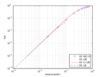
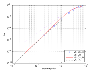
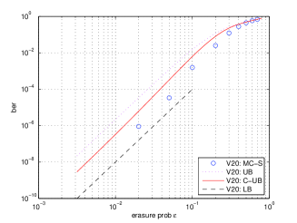
Figure 4: Comparisons among the upper bound (UB), the composite upper bound (C-UB), the Monte-Carlo simulation (MC-S), and the side product tight lower bound (LB) for bits 0, 5, and 20 of the (23,12) binary Golay code. The corresponding asymptotic (order, multiplicity) pairs obtained by UB, C-UB, and the actual BER is are V0: $\{(3,10),(4,75),(4,75)\}$, V5: $\{(3,15),(4,50),(4,45)\}$, and V20: $\{(4,221),(4,27),(4,1)\}$.

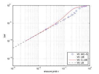
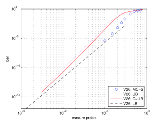
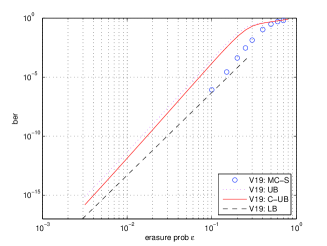
Figure 5: Comparisons among the UB, the C-UB, the MC-S, and the LB for bits 0, 26, and 19 of a randomly generated (3,6) LDPC code with $n=50$. The asymptotic (order, multiplicity) pairs of the UB, the C-UB, and the actual BER are V0: $\{(4,1),(4,1),(4,1)\}$, V26: $\{(6,2),(6,4),(6,2)\}$, and V19: $\{(7,135),(7,10),(7,5)\}$.

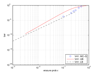
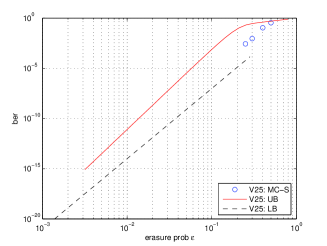
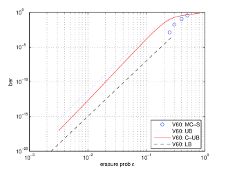
Figure 6: Comparisons among the UB, the C-UB, the MC-S, and the LB for bits 41, 25, and 60 of a randomly generated (3,6) LDPC code with $n=72$. The asymptotic (order, multiplicity) pairs of the UB, the C-UB, and the actual BER are V41: $\{(4,1),-,(4,1)\}$, V25: $\{(7,1),-,(7,1)\}$, and V60: $\{(7,19),(8,431),(8,11)\}$.

IV-E Performance

IV-E1 The (23,12) Binary Golay Code

The standard parity check matrix of the Golay code is considered. Fig. 4 compares the upper bound (UB), the composite upper bound (C-UB), the Monte-Carlo simulation (MC-S), and the side product, the tight lower bound (LB), on bits 0, 5, and 20. As illustrated, C-UB and LB tightly bracket the MC-S results, which shows that our UB and C-UB are capable of decoupling even non-sparse Tanner graphs with plenty of cycles.

IV-E2 A (3,6) LDPC Code with $n=50$

A (3,6) LDPC code with $n=50$ is randomly generated, and the UB, the C-UB, the MC-S, and the tight LB are performed on bits 0, 26, and 19, as plotted in Fig. 5, and the statistics of all 50 bits are provided in TABLE I(a). Our UB is tight in the asymptotic order for all bits while 34 bits are tight in multiplicity. Among the 16 bits not tight in multiplicity, 11 bits are within a factor of three of the actual multiplicity. In contrast with the Golay code example, the tight performance can be attributed to the sparse connectivity of the corresponding Tanner graph. As can be seen in Fig. 5(c), the C-UB possesses the greatest advantage over those UBs without tight multiplicity. The C-UB and the LB again tightly bracket the asymptotic performance.

IV-E3 A (3,6) LDPC Code with $n=72$

The UB, the C-UB, the MC-S, and the tight LB are applied to bits 41, 25, and 60, as plotted in Fig. 6 and the statistics are in TABLE I(b). Almost all asymptotic orders can be captured by the UB with only two exception bits. Both of the exception bits are of order 8, which is computed by applying the C-UB to each bit respectively.

IV-E4 (3,6) LDPC Codes with $n=144$

Complete statistics are presented in TABLE I(c), and we start to see many examples (101 out of 144 bits) in which our simple UB is not able to capture the asymptotic order. For those bits, we have to resort to the C-UB for tighter results. It is worth noting that the simple UB is able to identify some bits with order 9, which requires ${144\choose 9}=5.7\times 10^{13}$ trials if a brute force method is employed. Furthermore, all stopping sets of size $\leq 7$ have been identified, which shows that Algorithm 1 is able to generate tight ${\mathrm{UB}}$s when only FERs are considered. Among all our experiments, many of which are not reported herein, the most computationally friendly case is when considering FERs for irregular codes with many degree 2 variable nodes, which are one of the most important subjects of current research. In these scenarios, all stopping sets of size $\leq 13$ have been identified for non-trivial irregular codes with $n=576$, which evidences the superior efficiency of the proposed algorithm.

V Conclusion & Future Directions

A new technique upper bounding the BER of any finite code on BECs has been established, which, to our knowledge, is the first algorithmic result guaranteeing finite code performance while admitting efficient implementation. Preserving much of the decoding tree structure, this bound corresponds to a narrowing search of stopping sets. The asymptotic tightness of this technique has been proved, while the experiments demonstrate the inherent efficiency of this method for codes of moderate sizes $n\leq 300$. One major application of this upper bound is to design high rate codes with guaranteed asymptotic performance, and our results specify both the attainable low BER, e.g., $10^{-15}$, and at what SNR it can be achieved. One further research direction is on extending the setting to binary symmetric channels with quantized belief propagation decoders such as Gallager’s decoding algorithms A and B.

References

- [1] J. S. Yedidia, E. B. Sudderth, and J.-P. Bouchaud, “Projection algebra analysis of error correcting codes,” Mitsubishi Electric Research Laboratories, Technical Report TR2001-35, 2001.
- [2] T. Richardson, “Error floors of LDPC codes,” in Proc. 41st Annual Allerton Conf. on Comm., Contr., and Computing. Monticello, IL, USA, 2003.
- [3] R. Holzlöhner, A. Mahadevan, C. R. Menyuk, J. M. Morris, and J. Zweck, “Evaluation of the very low BER of FEC codes using dual adpative importance sampling,” IEEE Commun. Letters, vol. 9, no. 2, pp. 163–165, Feb. 2005.
- [4] K. M. Krishnan and P. Shankar, “On the complexity of finding stopping distance in Tanner graphs,” preprint.
- [5] A. Amraoui, R. Urbanke, A. Montanari, and T. Richardson, “Further results on finite-length scaling for iteratively decoded LDPC ensembles,” in Proc. IEEE Int’l. Symp. Inform. Theory. Chicago, 2004.
- [6] C. Di, D. Proietti, E. Telatar, T. J. Richardson, and R. L. Urbanke, “Finite-length analysis of low-density parity-check codes on the binary erasure channel,” IEEE Trans. Inform. Theory, vol. 48, no. 6, pp. 1570–1579, June 2002.
- [7] M. G. Stepanov, V. Chernyak, M. Chertkov, and B. Vasic, “Diagnosis of weaknesses in modern error correction codes: a physics approach,” Phys. Rev. Lett., to be published.