The Complexity of Mean Flow Time Scheduling Problems
with Release Times

Abstract

We study the problem of preemptive scheduling $n$ jobs with given release times on $m$ identical parallel machines. The objective is to minimize the average flow time. We show that when all jobs have equal processing times then the problem can be solved in polynomial time using linear programming. Our algorithm can also be applied to the open-shop problem with release times and unit processing times. For the general case (when processing times are arbitrary), we show that the problem is unary NP-hard.

1 Introduction

In the scheduling problem we study, the input instance consists of $n$ jobs with given release times and processing times. The objective is to compute a preemptive schedule of those jobs on $m$ machines that minimizes the average flow time or, equivalently, the sum of completion times, $\sum C_{j}$. In the standard scheduling notation, the problem can be described as $P|r_{j},{\mbox{\rm pmtn}}|\sum C_{j}$.

First, we focus on the case when all jobs have the same processing time $p$, that is $P|r_{j},p_{j}=p,{\mbox{\rm pmtn}}|\sum C_{j}$. Herrbach and Leung [4] showed that, for $m=2$, the optimal schedule can be computed in time $O(n\log n)$. For more machines, the complexity of the problem was open. Addressing this open problem, we present an algorithm whose running time is polynomial in $m$ and $n$.

Our algorithm is based on linear programming. We show that there is always an optimal schedule in a certain normal form. We then give a simple linear program of size $O(mn)$, which directly defines an optimal normal schedule. Since the coefficients in the constraints of our linear program are $-1$, $0$, or $1$, the result of Tardos [8] implies that the problem can be solved in worst case time $O(n^{5}m^{5})$.

We show that, without loss of generality, we can assume that the preemptions occur only at integer times. This yields a polynomial-time algorithm for the open shop problem $O|r_{i},p_{ij}=1|\sum C_{i}$, for it is known that this problem is equivalent to $P|r_{i},p_{i}=m,\mbox{pmtn}^{+}|\sum C_{i},$ where $m$ is the number of machines [2]. (Notation $\mbox{pmtn}^{+}$ means that preemptions are allowed only at integer times.) Previously, it was only known that this problem can be solved in polynomial time if $m$ is constant [9].

In the open shop problem $O|r_{i},p_{ij}=1|\sum C_{i}$ each job has to be processed on each machine exactly once and with a unit processing time. At any time each machine can execute at most one job and every job can be scheduled by at most one machine. No job can start before its given release time, and the goal is to minimize the total completion time.

In the last section we consider the general case, when the processing times are arbitrary. Du, Leung and Young [3] proved this problem is binary NP-hard for two machines. We show that if the number of machines is not fixed then the problem is in fact unary NP-complete.

We summarize the results discussed above in Table 1.

Problem	Complexity
$P2|r_{j};{\mbox{\rm pmtn}};p_{j}=p|\sum C_{j}$	solvable in time $O(n\log n)$ [4]
$P\phantom{2}|r_{j};{\mbox{\rm pmtn}};p_{j}=p|\sum C_{j}$	solvable in polynomial time [this paper]
$P2|r_{j};{\mbox{\rm pmtn}}\,\phantom{\;p_{j}=p}|\sum C_{j}$	binary NP-hard [3]
$P\phantom{2}|r_{j};{\mbox{\rm pmtn}}\,\phantom{\;p_{j}=p}|\sum C_{j}$	unary NP-complete [this paper]
$P\phantom{2}|\phantom{r_{j};}\,{\mbox{\rm pmtn}};p_{j}=p|\sum C_{j}$	solvable by the greedy algorithm (trivial)
$P\phantom{2}|r_{j};\phantom{{\mbox{\rm pmtn}}\;}\,p_{j}=p|\sum C_{j}$	solvable by the greedy algorithm (trivial)
$1\phantom{P}|r_{j};{\mbox{\rm pmtn}};p_{j}=p|\sum w_{j}C_{j}$	open
$P\phantom{2}|r_{j};{\mbox{\rm pmtn}};p_{j}=p|\sum w_{j}C_{j}$	unary NP-complete [6]
$O\phantom{2}|r_{j};\phantom{{\mbox{\rm pmtn}}\;}\,p_{ji}=1|\sum C_{j}$	solvable in $O(n^{2}m^{6m})$ [9], in polynomial time [this paper]

Table 1: Complexity of related scheduling problems. $P2$ stands for the two-machine problem, and $O$ for the open-shop problem. In problems with the objective function $\sum w_{j}C_{j}$, each job $j$ is assigned a weight $w_{j}\geq 0$, and the goal is to minimize the weighted sum of all completion times.

2 Structural Properties

Basic definitions.

Throughout the paper, $n$ and $m$ denote, respectively, the number of jobs and the number of machines. The jobs are numbered $1,2,\dots,n$ and the machines are numbered $1,2,\dots,m$. All jobs have the same length $p$. For each job $j$, $r_{j}$ is the release time of $j$, where, without loss of generality, we assume that $0=r_{1}\leq\ldots\leq r_{n}$. In this section we assume that all numbers $p,r_{1},\ldots,r_{n}$ are integers; in the appendix we show that our results can be extended to arbitrary real numbers.

We define a schedule ${\cal X}$ to be a function which, for any time $t$, determines the set ${\cal X}(t)$ of jobs that are running at time $t$. This set ${\cal X}(t)$ is called the profile at time $t$. Let ${\cal X}^{-1}(j)$ denote the set of times when $j$ is executed, that is ${\cal X}^{-1}(j)={\left\{t:j\in{\cal X}(t)\right\}}$. In addition we require that ${\cal X}$ satisfies the following conditions:

(s1) At most $m$ jobs are executed at any time, that is $|{\cal X}(t)|\leq m$ for all times $t$.

(s2) No job is executed before its release time, that is, for each job $j$, if $t<r_{j}$ then $j\notin{\cal X}(t)$.

(s3) Each job runs in a finite number of time intervals. More specifically, for each job $j$, ${\cal X}^{-1}(j)$ is a finite union of intervals of type $[s,t)$.

(s4) Each job is executed for time $p$, that is $|{\cal X}^{-1}(j)|=p$.

In (s4), for a set $X$ of real numbers we use $|X|$ to denote its measure. It is not difficult to see that condition (s3) can be relaxed to allow jobs to be executed in infinitely (but countably) many intervals, without changing the value of the objective function.

By $C_{j}=\sup{\cal X}^{-1}(j)$ we denote the completion time of a job $j$. In this paper, we are interested in computing a schedule that minimizes the objective function $\sum_{j=1}^{n}C_{j}$.

Note that, since we are dealing with preemptive schedules, it does not matter to which specific machines the jobs in ${\cal X}(t)$ are assigned to. When such an assignment is needed, we will use the convention that the jobs are assigned to machines in the increasing order of indices (or, equivalently, release times): the job with minimum index is assigned to machine $1$, the second smallest job to machine $2$, etc.

Integral schedules.

We say that a schedule ${\cal X}$ is integral, if ${\cal X}(t)$ is constant for $t\in[s,s+1)$ at any $s\in\mathbb{N}$. (In other words, all preemptions occur at integer times.) The following lemma is due to [1], and we include it here for the sake of completeness.

Lemma 1

There exists an optimal schedule ${\cal X}$ that is integral.

Proof: Let ${\cal X}$ be an arbitrary optimal schedule. We will show that there is an integral schedule ${\cal X}^{\prime}$ whose objective value is not greater than that of ${\cal X}$. The proof is based on a flow network model of the scheduling problem, and uses the fact that if all capacities are integral then there is an integral solution.

Let $C_{1},\ldots,C_{n}$ be the completion times in ${\cal X}$. We consider the set of all time points

$$\{r_{1},\ldots,r_{n},\lfloor C_{1}\rfloor,\lceil C_{1}\rceil,\ldots,\lfloor C_{n}\rfloor,\lceil C_{n}\rceil\}.$$

Suppose that there are $k$ distinct numbers in this set. We rename these numbers $t_{1},...,t_{k}$ and order them in increasing order, $t_{1}<\ldots<t_{k}$. These numbers define $k-1$ intervals $[t_{i},t_{i+1})$ for $1\leq i<k$.

We define a network which consists of the nodes $u_{1},\ldots,u_{n},v_{1},\ldots,v_{k-1}$, plus two more nodes designated as the source and the sink. A node $u_{j}$ represents job $j$ and a node $v_{i}$ represents interval $[t_{i},t_{i+1})$. For every job $j$, there is an arc from the source to $u_{j}$ with capacity $p$ and cost $0$. For every time interval $[t_{i},t_{i+1})$ there is an arc from $v_{i}$ to the sink with capacity $m(t_{i+1}-t_{i})$ and cost $0$. For every job $j$ and every interval $[t_{i},t_{i+1})\subseteq[r_{j},\lfloor C_{j}\rfloor)$, there is an arc from $u_{j}$ to $v_{i}$ with capacity $t_{i+1}-t_{i}$ and cost $0$. In addition, for every job $j$ for which $C_{j}$ is not integral, there is an arc from $u_{j}$ to $v_{i}$ for $t_{i}=\lfloor C_{j}\rfloor$ with capacity $1$ and cost $1$. (These are the only arcs with non zero cost.)

The schedule ${\cal X}$ corresponds to a flow of value $np$, where the flow on an arc $(u_{j},v_{i})$ has value $|{\cal X}^{-1}(j)\cap[t_{i},t_{i+1})|$. The flows on other arcs are uniquely determined by the flows on all arcs $[u_{j},v_{i})$. The cost of this flow is $w=\sum_{j=1}^{n}(C_{j}-\lfloor C_{j}\rfloor)$.

Now we consider the minimum cost flow with maximal value $np$ in this network. Let its cost be $w^{\prime}\leq w$. This minimum cost flow corresponds to a schedule ${\cal X}^{\prime}$ in the following manner. For each given $i$, the amount of each job $j$ scheduled in interval $[t_{i},t_{i+1})$ is equal to the flow on the arc $(u_{j},v_{i})$, which is bounded by the capacity $\ell=t_{i+1}-t_{i}$ of this arc. The total processing time $m\ell$ in this interval is assigned to jobs $1,2,\dots,n$, in this order, processor by processor, and for each processor from left to right. Since each $(u_{j},v_{i})$ has capacity $\ell$, a job will not be scheduled at two processors at the same time. Also, since the capacity of the arc between $v_{i}$ and the sink is $m\ell$, all jobs will be allocated the required processing time.

Since all arcs have integer capacity, the minimum cost flow can be assumed to be integer (see [7].) Therefore the resulting schedule ${\cal X}^{\prime}$ is integral. It remains to show that its objective value is not larger than that of ${\cal X}$.

For each job $j$, let $C^{\prime}_{j}$ be the completion time of $j$ in ${\cal X}^{\prime}$. By the construction of the network, we have $C^{\prime}_{j}\leq\lceil C_{j}\rceil$. Moreover, for $w^{\prime}$ jobs $j$ we have $C^{\prime}_{j}=\lceil C_{j}\rceil>\lfloor C_{j}\rfloor$, and for these jobs $C_{j}$ is not integer, while for all the other $n-w^{\prime}$ jobs $j$ we have $C^{\prime}_{j}\leq\lfloor C_{j}\rfloor$. Setting $\tilde{C}=\sum_{j=1}^{n}\lfloor C_{j}\rfloor$, the cost of ${\cal X}^{\prime}$ is

$$\sum_{j=1}^{n}C^{\prime}_{j}\;\leq\;\tilde{C}+w^{\prime}\;\leq\;\tilde{C}+w\;\leq\;\tilde{C}+\sum_{j=1}^{n}(C_{j}-\lfloor C_{j}\rfloor)\;=\;\sum_{j=1}^{n}C_{j},$$

completing the proof of the lemma. $\Box$

Busy schedules.

We now show that, for the purpose of minimizing our objective function, we can restrict our attention to schedules with some additional properties.

We say that a schedule ${\cal X}$ is busy if it satisfies the following condition: for any two times $s<t$ and a job $j$ such that $r_{j}\leq s$, if $j\in{\cal X}(t)$ and $|{\cal X}(s)|<m$ (that is, some machine is idle at $s$) then $j\in{\cal X}(s)$ as well. Any optimal schedule is busy, for otherwise, if the above condition is not satisfied, we can move a sufficiently small portion $\epsilon>0$ of $j$ from the last block where it is executed to the interval $[s,s+\epsilon)$, obtaining a feasible schedule in which the completion time of $j$ is reduced by $\epsilon$ and other completion times do not change. Thus we only need to be concerned with busy schedules.

Reductions.

Let ${\cal X}$ be a schedule, and $i,j$ be two jobs with $r_{i}<r_{j}$. Let $T$ be the set of times where exactly one of the jobs $i,j$ is scheduled, that is $T=[{\cal X}^{-1}(i)\setminus{\cal X}^{-1}(j)]\cup[{\cal X}^{-1}(j)\setminus{\cal X}^{-1}(i)]$. Also, let $t_{0}$ be a time point which divides $T$ into two parts of the same size, that is $|T\cap[0,t_{0})|=\frac{1}{2}|T|$. Since $i$ and $j$ have equal processing time, the processing times of each of $i$ and $j$ in $T$ is equal $\frac{1}{2}|T|$. The $(i,j)$-reduction modifies the schedule by executing $i$ in $|T\cap[0,t_{0})|$ and $j$ in $T\cap[t_{0},\infty)$. If the reduction does not change ${\cal X}$ (that is, $i$ is executed in $|T\cap[0,t_{0})|$ and $j$ in $T\cap[t_{0},\infty)$) then we say that $i$ and $j$ are in order.

We say that a schedule ${\cal X}$ is irreducible if it is busy and all pairs of jobs are in order. It is not difficult to see that ${\cal X}$ is irreducible iff it satisfies the following condition for any times $s<t$:

$$\max(\,{\cal X}(s)-{\cal X}(t)\,) < \min(\,{\cal X}(t)-{\cal X}(s)\,),$$ (1)

where the order refers to job indices, which we assumed to satisfy $i<j\Rightarrow r_{i}\leq r_{j}$. Also, we use the convention that $\max(\emptyset)=-\infty$ and $\min(\emptyset)=+\infty$, so (1) holds whenever ${\cal X}(s)\subseteq{\cal X}(t)$ or ${\cal X}(t)\subseteq{\cal X}(s)$.

Lemma 2

For any two jobs $i,j$ with $r_{i}<r_{j}$, an $(i,j)$-reduction of ${\cal X}$ does not increase the objective function, and preserves the integrality and the property of being busy.

Proof: In the $(i,j)$-reduction, only the completion times of $i$ and $j$ might change. Let $C_{i},C_{j}$ be the completion times of $i$, $j$, before the reduction and $C^{\prime}_{i},C^{\prime}_{j}$ after the reduction. We have three cases. If $C_{i}>C_{j}$ then $C^{\prime}_{j}=C_{i}$ and $C^{\prime}_{i}\leq C_{j}$. If $C_{i}=C_{j}$, then the completion times do not change. If $C_{i}<C_{j}$, then $C^{\prime}_{j}=C_{j}$ and $C^{\prime}_{i}\leq C_{i}$. Thus in all three cases $C_{i}+C_{j}$ does not increase.

To justify the second part of the lemma, note that the reduction does not change the cardinality of ${\cal X}(t)$ at any time point $t$. Therefore the new schedule remains busy. Further, if ${\cal X}$ is integral then $t_{0}$ can be assumed to be an integer, and the new schedule will then be integral as well. $\Box$

Theorem 3

There is an optimal schedule ${\cal X}$ that is irreducible.

Proof: Let ${\cal X}$ be an optimal schedule that is busy and integral. We define a potential function which decreases strictly when a reduction of two jobs which are not in order is applied. From this we conclude that after a finite number of reductions we must reach an irreducible schedule.

Define $H({\cal X})=(H_{1}({\cal X}),H_{2}({\cal X}),\ldots,H_{n}({\cal X}))$, where $H_{j}({\cal X})=\sum_{t\in\mathbb{N},t\in{\cal X}^{-1}(j)}t$ for each job $j$. Given two different schedules ${\cal X}$, ${\cal Y}$, we say that $H({\cal X})$ is lexicographically smaller than $H({\cal Y})$, if $H_{i}({\cal X})<H_{i}({\cal Y})$ for the smallest $i$ for which $H_{i}({\cal X})\neq H_{i}({\cal Y})$.

If two jobs $i<j$ are not in order, then the $(i,j)$-reduction decreases $H_{i}({\cal X})$, while $H_{j}({\cal X})$ increases. Therefore $H({\cal X})$ decreases lexicographically. Any value $H_{j}({\cal X})$ is integer and bounded by $0\leq H_{j}({\cal X})\leq p(\max_{i}C_{i})$, where $\max_{i}C_{i}$ is preserved by the reductions. From this we can conclude that after a finite number of reductions we obtain an irreducible optimal schedule. $\Box$

We now give a characterization of irreducible schedules that will play a major role in the construction of our linear program.

For a given job $j$ and a time $t$ we partition ${\cal X}(t)-{\left\{j\right\}}$ into jobs released before and after $j$. Formally, ${\cal X}_{<j}(t)={\left\{i\in{\cal X}(t):i<j\right\}}$ and ${\cal X}_{>j}(t)={\left\{i\in{\cal X}(t):i>j\right\}}$. The lemma below provides a characterization of irreducible schedules. (See Figure 1.)

Figure 1: Structure of any irreducible schedule.

Lemma 4

Let ${\cal X}$ be an irreducible schedule. Let $u,t$ be two time points and $k$ be a job such that $r_{k}\leq u<t$. Then:

(a) If $k\in{\cal X}(u)-{\cal X}(t)$ then $|{\cal X}_{<k}(t)|\leq|{\cal X}_{<k}(u)|$.

(b) If $k\in{\cal X}(t)-{\cal X}(u)$ then $|{\cal X}(u)|=m$, $|{\cal X}_{>k}(t)|\geq|{\cal X}_{>k}(u)|$, and $|{\cal X}_{<k}(t)|<|{\cal X}_{<k}(u)|$.

(c) If $k\in{\cal X}(u)\cap{\cal X}(t)$ then $|{\cal X}_{<k}(t)|\leq|{\cal X}_{<k}(u)|$ and $|{\cal X}_{>k}(t)|\geq|{\cal X}_{>k}(u)|$.

Proof: Case (a) $k\in{\cal X}(u)-{\cal X}(t)$: We will show by contradiction that ${\cal X}_{<k}(t)\subseteq{\cal X}_{<k}(u)$, so suppose that there is a job $j\in{\cal X}_{<k}(t)-{\cal X}_{<k}(u)$. Then $j\geq\min({\cal X}_{<k}(t)-{\cal X}_{<k}(u))=\min({\cal X}(t)-{\cal X}(u))$. Also $j<k$, and $k\leq\max({\cal X}(u)-{\cal X}(t))$. This contradicts irreducibility by equation (1) and thus (a) follows.

Case (b) $k\in{\cal X}(t)-{\cal X}(u)$: Since $k\not\in{\cal X}(u)$ and $r_{k}\leq u$, the assumption that ${\cal X}$ is busy implies that $|{\cal X}(u)|=m$.

We must have ${\cal X}_{>k}(u)\subseteq{\cal X}_{>k}(t)$, for otherwise, the existence of $k\in{\cal X}(t)-{\cal X}(u)$ and an $l\in{\cal X}_{>k}(u)-{\cal X}_{>k}(t)$ would contradict irreducibility. The inequality $|{\cal X}_{>k}(u)|\leq|{\cal X}_{>k}(t)|$ follows. This, the assumption of the case, and $|{\cal X}(u)|=m$ imply $|{\cal X}_{<k}(u)|>|{\cal X}_{<k}(t)|$.

Case (c) $k\in{\cal X}(u)\cap{\cal X}(t)$: We only prove the first inequality, as the proof for the second one is very similar. Towards contradiction, suppose $|{\cal X}_{<k}(u)|<|{\cal X}_{<k}(t)|$, and pick any $i\in{\cal X}_{<k}(t)-{\cal X}_{<k}(u)$. Then $r_{i}\leq r_{k}\leq u$ and $i\in{\cal X}(t)-{\cal X}(u)$, and so the assumption that ${\cal X}$ is busy implies ${\cal X}(u)=m$. This, in turn, implies that $|{\cal X}_{>k}(u)|>|{\cal X}_{>k}(t)|$, so we can choose $j\in{\cal X}_{>k}(u)-{\cal X}_{>k}(t)$. But this means that $j>k>i$ and $j\in{\cal X}(u)-{\cal X}(t)$, and the existence of such $i$ and $j$ contradicts irreducibility. $\Box$

3 A Linear Program for $P|r_{j};{\mbox{\rm pmtn}};p_{j}=p|\sum C_{j}$

Machine assignment.

We now consider the actual job-machine assignment in an irreducible schedule ${\cal X}$. As explained earlier, at every time $t$ we assign the jobs in ${\cal X}(t)$ to machines in order, that is job $j\in{\cal X}(t)$ is assigned to machine $1+|{\cal X}_{<j}(t)|$. Lemma 4 implies that, for any fixed $j$, starting at $t=r_{j}$ the value of $|{\cal X}_{<j}(t)|$ decreases monotonically with $t$. Therefore, with machine assignments taken into account, ${\cal X}$ will have the structure illustrated in Figure 1.

Call a schedule ${\cal X}$ normal if for each job $j$ and each machine $q$, job $j$ is executed on $q$ in a single (possibly empty) interval $[S_{j,q},C_{j,q})$, and

(1) $C_{j,q}\leq S_{j+1,q}$ for each machine $q$ and job $j<n$, and

(2) $C_{j,q}\leq S_{j,q-1}$ for each machine $q>1$ and job $j$.

By the earlier discussion, every irreducible schedule is normal (although the reverse does not hold.) An example of a normal (and irreducible) schedule is shown in Figure 2.

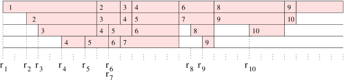
Figure 2: Example of a normal schedule. The processing time is $p=8$.

Linear program.

We are now ready to construct our linear program:

minimize $$\textstyle{\sum_{j=1}^{n}C_{j,1}}$$ (2)

subject to $$-S_{j,m}\; \leq-r_{j} j=1,\dots,n$$

$$\sum_{q}(C_{j,q}-S_{j,q})\; =p j=1,\dots,n$$

$$S_{j,q}-C_{j,q}\; \leq 0 j=1,\dots,n,\;q=1,\dots,m$$

$$C_{j,q}-S_{j,q-1}\; \leq 0 j=1,\dots,n,\;q=2,\dots,m$$

$$C_{j,q}-S_{j+1,q}\; \leq 0 j=1,\dots,n-1,\;q=1,\dots,m$$

The correspondence between normal schedules and feasible solutions to this linear program should be obvious. For any normal schedule, the start times $S_{j,q}$ and completion times $C_{j,q}$ satisfy the constraints of (2). And vice versa, for any set of the numbers $S_{j,q}$, $C_{j,q}$ that satisfy the constraints of (2), we get a normal schedule by scheduling any job $j$ in interval $[S_{j,q},C_{j,q})$ on each machine $q$. Thus we can identify normal schedules ${\cal X}$ with feasible solutions of (2). Note, however, that in ${\cal X}$ a job $j$ could complete earlier than $C_{j,1}$ (this can happen when $C_{j,1}=S_{j,1}$.) Thus the only remaining issue is whether the optimal normal schedules correspond to optimal solutions of (2).

Theorem 5

The linear program above correctly computes an optimal schedule. More specifically, $\min_{\cal X}\sum_{j}C_{j}=\min\sum_{j}C_{j,1}$, where on the left-hand side the minimum is over normal schedules ${\cal X}$ with $C_{j}$ representing the completion time of job $j$ in ${\cal X}$, and on the right-hand side we have the optimal solution of the linear program (2).

Proof: $(\leq)$ By the correspondence between normal schedules and feasible solutions of (2), discussed before the theorem, we have $C_{j}\leq C_{j,1}$ for all $j$, and thus the $\leq$ inequality is trivial.

$(\geq)$ To justify the other inequality, fix an optimal irreducible (and thus also normal) schedule ${\cal X}$. We want to show a feasible solution to (2) for which $C_{j}=C_{j,1}$ for all $j$.

Fix a job $j$, and let $[S_{j,g},C_{j,g})$ be the last (that is, the one with minimum $g$) non-empty execution interval of $j$. So $C_{j}=C_{j,g}$ in ${\cal X}$. Consider a block $[s,t)$ where $t=C_{j,g}$. By Lemma 4, all jobs executed on machines $1,2,\dots,g-1$ in $[s,t)$ are numbered lower than $j$. Further, by the ordering of completion times, they are not executed after $t$. Thus these jobs must be completed at $t$ as well. Therefore we can set $[S_{j,h},C_{j,h})=[t,t)$, for all machines $1\leq h<g$. This gives a normal schedule in which $C_{j}=C_{j,1}$.

Having done this for all jobs, we will get numbers $S_{j,q}$ and $C_{j,q}$ that satisfy all constraints of the linear program, and such that $C_{j}=C_{j,1}$ for all $j$. $\Box$

4 Unary NP-Hardness of $P|r_{j},\mbox{\rm pmtn}|\sum C_{j}$

In this section we prove that without the assumption on equal processing times the problem is strongly (unary) NP-hard.

Theorem 6

The problem $P|r_{j},\mbox{\rm pmtn}|\sum C_{j}$ is strongly NP-hard, that is, it is NP-hard even if the numbers on input are represented in the unary encoding.

Proof: The proof is by reduction from 3-Partition. In an instance ${\cal I}$ of 3-Partition we have $3n+1$ numbers $x_{1},x_{2},\dots,x_{3n},y$ such that $\sum_{i=1}^{3n}x_{i}=ny$ and ${\mbox{$\frac{1}{4}$}}y<x_{i}<{\mbox{$\frac{1}{2}$}}y$ for each $i$. We want to determine whether there is a partition of ${\left\{1,2,\dots,3n\right\}}$ into $n$ sets $S_{1},\dots,S_{n}$ such that $\sum_{i\in S_{k}}x_{i}=y$ for all $k$. (By the assumption about the numbers $x_{i}$, in any such partition all sets $S_{k}$ have exactly three elements.)

Given an instance of 3-Partition above, we construct an instance ${\cal J}$ of $P|r_{j},\mbox{\rm pmtn}|\sum C_{j}$ as follows. Define $A=6ny$ and $B=18n^{2}y^{2}$. We let $m=n$, and $N=4n+An$. We create three types of jobs:

x-jobs:

For each $j=1,\dots,3n$, we create job $j$ with $r_{j}=0$ and $p_{j}=Ax_{j}$.

B-jobs:

For each $j=3n+1,\dots,4n$, we create job $j$ with $r_{j}=Ay$ and $p_{j}=B$.

1-jobs:

For each $j=4n+1,\dots,N$, we create job $j$ with $r_{j}=Ay+B$ and $p_{j}=1$.

If ${\cal I}$ is represented in unary, its size is $\Theta(ny)$. Then the size of ${\cal J}$ (in unary encoding) is polynomial and the above transformation works in polynomial time.

Thus now it is sufficient to prove the following claim: ${\cal I}$ has a 3-partition if and only if ${\cal J}$ has a schedule with $\sum_{j=1}^{N}C_{j}\leq D$, where $D=3nAy+n(Ay+B)+n\sum_{i=1}^{A}(Ay+B+i)$.

$(\Rightarrow)$ Let $S_{1},\dots,S_{n}$ be a 3-partition of ${\cal I}$. For each $k$ we have $\sum_{j\in S_{k}}p_{j}=Ay$. So on machine $k$ we schedule the following jobs: first the three x-jobs $j\in S_{k}$, completing the last one at $Ay$, then one B-job, followed by $A$ 1-jobs. The objective value of this schedule is

$$\sum_{j=1}^{N}C_{j} \leq 3nAy+n(Ay+B)+n\sum_{i=1}^{A}(Ay+B+i)\;=\;D.$$

$(\Leftarrow)$ Suppose now that ${\cal I}$ does not have a 3-partition. Consider any schedule ${\cal X}$ of ${\cal J}$ on $n$ machines. We want to prove that the value of the objective function for ${\cal X}$ exceeds $D$.

We consider easy cases first. If some x-job is completed after time $Ay+B$ then

$$\sum_{j=1}^{N}C_{j} > Ay+B+n(Ay+B)+n\sum_{i=1}^{A}(Ay+B+i)\;>\;D.$$

If some B-job is completed after time $Ay+2B$ then

$$\sum_{j=1}^{N}C_{j} > (n-1)(Ay+B)+Ay+2B+n\sum_{i=1}^{A}(Ay+B+i)\;\geq\;D.$$

Suppose now that each x-job is completed no later than at time $Ay+B$ and each B-job is completed no later than at time $Ay+2B$. Since ${\cal I}$ does not have a 3-partition, some machine is idle for $A$ time units in the interval $[0,Ay]$. Therefore some B-job will complete between $Ay+B+A$ and $Ay+2B$, keeping one machine busy in the interval $[Ay+B,Ay+B+A]$. This implies that there are at least $A$ 1-jobs that will be scheduled at time $Ay+A+B$ or later. Thus

$$\sum_{j=1}^{N}C_{j} > (n-1)(Ay+B)+Ay+A+B+(n-1)\sum_{i=1}^{A}(Ay+B+i)+A(Ay+A+B)\;>\;D.$$

Summarizing, in all cases the objective value exceeds $D$, completing the proof of the claim. $\Box$

5 Final Remarks

We proved that the scheduling problem $P|r_{j},{\mbox{\rm pmtn}},p_{j}=p|\sum C_{j}$ can be reduced to solving a linear program with $O(mn)$ variables and constraints. This leads to a simple polynomial time algorithm. Since we can assume that $m\leq n$ (otherwise the problem is trivial) the running time can be also expressed as a polynomial of $n$ only.

We showed that there is an optimal schedule with $O(mn)$ preemptions. We do not know whether this bound is asymptotically tight. It is quite possible that there exist optimal schedules in which the number of preemptions is $O(n)$, independent of $m$. If this is true, this could lead to even more efficient, combinatorial (not dependent on linear programming) algorithms for this problem. Such improvement, however, would require a deeper study of the structural properties of optimal schedules. Since we use only the existence of normal optimal schedules, rather than irreducible schedules, we feel that the problem has more structure to be exploited.

An interesting related open question is $P|r_{j},p_{j}=p|\sum U_{j}$, where the objective is to find a maximal subset of jobs which can be scheduled on time. It has been shown in [5] that the corresponding preemptive version, $P|r_{j},p_{j}=p,\mbox{pmtn}|\sum U_{j}$, is unary NP-hard.

We implemented the complete algorithm (converting the instance to a linear program and solving this linear program). It is accessible at Christoph Dürr’s webpage.

Appendix A Proof of Theorem 3 for Arbitrary Real Numbers

In Section 2 we proved that there is always an optimal irreducible schedule, under the assumption that the processing time $p$ and the release times $r_{1},\dots,r_{n}$ are integral. We now show that this is true in the more general scenario when all these numbers are arbitrary reals.

We first extend the definition of the potential function. For any job $j$, let ${\bar{H}}_{j}({\cal X})={\mbox{$\frac{1}{2}$}}\int_{{\cal X}^{-1}(j)}t\,\mathrm{d}t$, where the integral is taken over the support of $j$. (We remark that this is a standard value in scheduling, even though the factor $\frac{1}{2}$ is irrelevant for this paper.) The generalized potential function is ${\bar{H}}({\cal X})=({\bar{H}}_{1}({\cal X}),\ldots,{\bar{H}}_{n}({\cal X}))$.

The following properties remain true: (i) a reduction does not increase the objective function and preserves the property of a schedule being busy, (ii) ${\bar{H}}({\cal X})$ strictly decreases (lexicographically) after each reduction.

The major difficulty that we need to overcome is that the set of schedules is not closed as a topological space, so there could be a sequence of schedules with decreasing values of ${\bar{H}}({\cal X})$ whose limit is not a legal schedule. The idea of the proof is to reduce the problem to minimizing ${\bar{H}}({\cal X})$ over a compact subset of schedules.

Lemma 7

Even if $p,r_{1},\dots,r_{n}$ are arbitrary real numbers, there is an irreducible optimal schedule.

Proof: Define a block of a schedule ${\cal X}$ to be a maximal time interval $[u,t)$ such that $(u,t)$ does not contain any release times and ${\cal X}(s)$ is constant for $s\in[u,t)$.

For convenience, let $r_{n+1}$ be any upper bound on the last completion time of any optimal schedule, say $r_{n+1}=r_{n}+np$. Thus all jobs are executed between $r_{1}$ and $r_{n+1}$. Each interval $[r_{i},r_{i+1})$, for $i=1,\dots,n$ is called a segment. By condition (s3), each segment is a disjoint union of a finite number of blocks of ${\cal X}$. Also, for each job $j$, we have $C_{j}=t$ for the last non-empty block $[s,t)$ whose profile contains $j$.

A schedule ${\cal X}$ is called tidy if all jobs are completed no later than at $r_{n+1}$ and, for any segment $[r_{i},r_{i+1})$, the profiles ${\cal X}(t)$, for $t\in[r_{i},r_{i+1})$, are lexicographically ordered from left to right. More precisely, this means that, for any $r_{i}\leq s<t<r_{i+1}$, we have

$$\min(\,{\cal X}(s)-{\cal X}(t)\,) \leq \min(\,{\cal X}(t)-{\cal X}(s)\,).$$

One useful property of tidy schedules is that its total number of blocks (including the empty ones) is $N=nM$, where $M=\sum_{l=0}^{m}\binom{n}{l}$, because $n$ is the number of intervals $[r_{i},r_{i+1})$ and $M$ is the number of lexicographically ordered blocks in each interval. From now on we identify any tidy schedule ${\cal X}$ with the vector ${\cal X}\in\reals^{N}$ whose $b$-th coordinate $x_{b}$ represents the length of the $b$-th block in ${\cal X}$.

In fact, the set ${\bf T}$ of tidy schedules is a (compact) convex polyhedron in $\reals^{N}$, for we can describe ${\bf T}$ with a set of linear inequalities that express the following constraints:

• Each job $j$ is not executed before $r_{j}$,

• Each job $j$ is executed for time $p$.

For example, the second constraint can be written as $\sum_{b}x_{b}=p$, where the sum is over all blocks $b$ whose profile contains $j$.

Claim 8

Any schedule ${\cal X}$ can be transformed into a schedule with completion times ordered as $C_{1}\leq\ldots\leq C_{n}$, without increasing the objective function value.

Proof: Note that after an $(i,j)$-reduction we have $C_{i}\leq C_{j}$, and no other completion time is changed. Therefore after reducing job $1$ successively with the jobs $2,\ldots,n$, $C_{1}$ is the smallest completion time. Then after reducing job $2$ with the jobs $3,\ldots,n$ we have $C_{1}\leq C_{2}\leq\min\{C_{3},\ldots,C_{n}\}$. Continuing this process will eventually end with ordered completion times. $\Box$

Claim 9

Let ${\cal X}$ be a schedule in which completion times are ordered and upper bounded by $r_{n+1}$. Then ${\cal X}$ can be converted into a tidy schedule ${\cal X}^{\prime}$ such that

(a) $C^{\prime}_{j}\leq C_{j}$ for all $j$ (where $C_{j}$ and $C^{\prime}_{j}$ are the completion times of $j$ in ${\cal X}$ and ${\cal X}^{\prime}$, respectively.)

(b) ${\bar{H}}({\cal X}^{\prime})$ is equal to or lexicographically smaller than ${\bar{H}}({\cal X})$.

Proof: Indeed, suppose that ${\cal X}$ has two consecutive blocks $A=[u,s)$, $B=[s,t)$ where $r_{i}\leq u<s<t\leq r_{i+1}$, and the profile ${\cal X}(u)$ of $A$ is larger (lexicographically) than the profile ${\cal X}(s)$ of $B$. Exchange $A$ and $B$, and denote by ${\cal X}^{\prime}$ the resulting schedule. Let $j=\min({\cal X}(s)-{\cal X}(u))<\min({\cal X}(u)-{\cal X}(s))$. Since $C_{j}\geq t$, all jobs in ${\cal X}(u)-{\cal X}(s)$ are also completed not earlier than at $t$. So this exchange does not increase any completion times. We have ${\bar{H}}_{j}({\cal X}^{\prime})<{\bar{H}}_{j}({\cal X})$ and ${\bar{H}}_{i}({\cal X}^{\prime})={\bar{H}}_{i}({\cal X})$ for $i<j$. Thus ${\bar{H}}({\cal X}^{\prime})$ is lexicographically smaller than ${\bar{H}}({\cal X})$. By repeating this process, we eventually convert ${\cal X}$ into a tidy schedule that satisfies the claim. $\Box$

We now continue the proof of the lemma. Fix some optimal schedule ${\cal X}^{\ast}$. Let $C^{\ast}_{j}$ denote the completion time of a job $j$ in ${\cal X}^{\ast}$. From Claims 8 and 9, we can assume that ${\cal X}^{\ast}$ is tidy and $C^{\ast}_{1}\leq C^{\ast}_{2}\leq\ldots\leq C^{\ast}_{n}$. (For the peace of mind, it is worth noting that Claim 9 implies that ${\cal X}^{\ast}$ is well defined, for it reduces the problem to minimizing $\sum_{j}C_{j}$ over a compact subset ${\bf T}$ of $\reals^{N}$.)

Consider a class ${\bf T}_{0}\subseteq{\bf T}$ of tidy schedules ${\cal X}$ such that each job $j$ in ${\cal X}$ is completed not later than at time $C^{\ast}_{j}$. Since ${\cal X}^{\ast}\in{\bf T}_{0}$, the set ${\bf T}_{0}$ is not empty. Similarly as ${\bf T}$, ${\bf T}_{0}$ is a (compact) convex polyhedron. Indeed, we obtain ${\bf T}_{0}$ by using the same constraints as for ${\bf T}$ and adding the constraints that each job $j$ is completed not later than at $C^{\ast}_{j}$. To express this constraint, if in ${\cal X}^{\ast}$ the completion time $C^{\ast}_{j}$ of $j$ is at the end of the $a$-th block in the segment $[r_{i},r_{i+1})$, then for each $b>(i-1)M+a$ such that $j$ is in the profile of the $b$-th block, we would have a constraint $x_{b}=0$. Note that these constraints do not explicitly force $j$ to end exactly at $C^{\ast}_{j}$, but the optimality of ${\cal X}^{\ast}$ guarantees that it will have to.

Now we show that there exists a schedule ${\cal Y}^{\ast}\in{\bf T}_{0}$ for which ${\bar{H}}({\cal Y}^{\ast})$ is lexicographically minimum. First, as we explained earlier, ${\bf T}_{0}$ is a compact convex polyhedron. Let ${\bf T}_{1}\subseteq{\bf T}_{0}$ be the set of ${\cal X}$ for which ${\bar{H}}_{1}({\cal X})$ is minimized. ${\bar{H}}_{1}$ is a continuous quadratic function over ${\bf T}_{0}$, and thus ${\bf T}_{1}$ is also a non-empty compact set. Continuing this process, we construct sets ${\bf T}_{2},\ldots,{\bf T}_{n}$, and we choose ${\cal Y}^{\ast}$ arbitrarily from ${\bf T}_{n}$. $\Box$

References

- [1] Ph. Baptiste. Polynomial time algorithms for minimizing the weighted number of late jobs on a single machine when processing times are equal. Journal of Scheduling, 2:245–252, 1999.
- [2] P. Brucker, B. Jurisch, and M. Jurisch. Open shop problems with unit time operations. Zeitschrift für Operations Research, 37:59–73, 1993.
- [3] J. Du, J.Y.-T. Leung, and G.H. Young. Minimizing mean flow time with release time constraint. Theoretical Computer Science, 75:347–355, 1990.
- [4] L.A. Herrbach and J.Y.-T. Leung. Preemptive scheduling of equal length jobs on two machines to minimize mean flow time. Operations Research, 38:487–494, 1990.
- [5] S. A. Kravchenko. On the complexity of minimizing the number of late jobs in unit time open shop. Discrete Applied Mathematics, 100:127–132, 2000.
- [6] J.Y.-T. Leung and G.H. Young. Preemptive scheduling to minimize mean weighted flow time. Information Processing Letters, 34:47–50, 1990.
- [7] A. Schrijver. Combinatorial Optimization. Springer Verlag, 2003.
- [8] E. Tardos. A strongly polynomial algorithm to solve combinatorial linear programs. Operations Research, 34:250–256, 1986.
- [9] T. Tautenhahn and G. J. Woeginger. Minimizing the total completion time in a unit-time open shop with release times. Operations Research Letters, 20:207–212, 1997.