Analytic Properties and Covariance Functions of a New Class of Generalized Gibbs Random Fields

Abstract

Spartan Spatial Random Fields (SSRFs) are generalized Gibbs random fields, equipped with a coarse-graining kernel that acts as a low-pass filter for the fluctuations. SSRFs are defined by means of physically motivated spatial interactions and a small set of free parameters (interaction couplings). This paper focuses on the FGC-SSRF model, which is defined on the Euclidean space $\mathbb{R}^{d}$ by means of interactions proportional to the squares of the field realizations, as well as their gradient and curvature. The permissibility criteria of FGC-SSRFs are extended by considering the impact of a finite-bandwidth kernel. It is proved that the FGC-SSRFs are almost surely differentiable in the case of finite bandwidth. Asymptotic explicit expressions for the Spartan covariance function are derived for $d=1$ and $d=3$; both known and new covariance functions are obtained depending on the value of the FGC-SSRF shape parameter. Nonlinear dependence of the covariance integral scale on the FGC-SSRF characteristic length is established, and it is shown that the relation becomes linear asymptotically. The results presented in this paper are useful in random field parameter inference, as well as in spatial interpolation of irregularly-spaced samples.

I Introduction

Spatial Random Fields (SRF’s) have a wide range of applications in hydrological models [14, 26, 30], petroleum engineering [16], environmental data analysis [10, 36, 25], mining exploration and mineral reserves estimation [15, 4], environmental health [11], image analysis [41, 40], medical image registration [3] and brain research [34, 28, 9] among other fields.

A spatial random field $\{X({\bf s},\omega)\in\mathbb{R};\,{\bf s}\in D(L)\subset\mathbb{R}^{d};\omega\in\Omega\}$ is defined as a mapping from the probability space $(\Omega,A,P)$ into the space of real numbers so that for each fixed ${\bf s}$, $X({\bf s},\omega)$ is a measurable function of $\omega$ [1, p. 3]. $D(L)$ is the domain within which the SRF is defined and $L$ is a characteristic domain length. An SRF involves by definition many possible states [10, p. 27],[42], denoted by $\omega$. In the following, for notational simplicity we suppress the dependence on $\omega.$

Realization of a particular state is determined from a joint probability density function (p.d.f.) $f_{\rm x}\left[X({\bf s})\right]$. The p.d.f. depends on the spatial configuration of the field’s point values. For spatial data the term sample refers to $N$ values $X({\bf s}_{i})$ from a particular state at the measurement locations $\{{\bf s}_{i},\>i=1,\ldots,N\}$, representing a single state of the SRF (an observed realization).

For irregularly-spaced samples, practical applications involve determining the statistical parameters of spatial dependence and interpolating the data on a regular grid. An observed realization, $X^{*}({\bf s})$, can be decomposed into a deterministic trend $m_{\rm x}({\bf s})$, a correlated fluctuation SRF $X_{\lambda}({\bf s})$, and a random noise term, $e({\bf s}),$ i.e., $X^{*}({\bf s})=m_{\rm x}({\bf s})+X_{\lambda}({\bf s})+e({\bf s}).$ The trend is a non-stationary component representing large-scale, deterministic variations, which presumably correspond to the ensemble average of the SRF, i.e. $m_{\rm x}({\bf s})=E[X({\bf s})]$.

The fluctuation corresponds to variations that involve smaller spatial scales than the trend. It is assumed that resolvable fluctuations exceed the spatial resolution $\lambda$. The component $e({\bf s})$ represents inherent variability below the resolution cutoff, or completely random variability due to uncorrelated measurement errors. It will be assumed that $e({\bf s})$ is statistically independent of the SRF $X_{\lambda}({\bf s})$, and can be treated as Gaussian white noise.

It is assumed in the following that the trend has been estimated and removed. This work focuses on modeling the correlated fluctuations.

For many geostatistical applications, the fluctuation can be viewed as a weakly stationary SRF, or an intrinsic random field with second-order stationary increments [42, pp. 308-438],[29]. An SRF is weakly stationary if its expectation $m_{\rm x}({\bf s})$ is independent of the location, and its covariance function $G_{\rm x}({\bf s},{\bf s}+{\bf r})$ depends only on the spatial lag ${\bf r}$. In the following, the term ‘stationary’ will refer to weak stationarity.

Furthermore, a stationary SRF is statistically isotropic if the covariance function depends only on the Euclidean distance between points but not on the direction of the lag vector, i.e., $G_{\rm x}(|{\bf r}|)$, where $|{\bf r}|)$ is the Euclidean norm of the vector ${\bf r}$. The isotropic assumption is not restrictive, since the anisotropic parameters can be inferred from the data and isotropy can be restored by rotation and rescaling transformations [17, 20, 13, 21].

For isotropic, short-ranged SRF’s, one can define a single integral scale [30, p. 22], given by the integral of the covariance function along any direction in space. Since the parameters of the fluctuation SRF are determined from the available sample by employing the ergodic hypothesis [42, p. 29],[27, p. 30], the integral scale must be considerably smaller than the domain size $L$.

The distribution of Gibbs random fields is expressed in terms of an energy functional $H[X_{\lambda}({\bf s});{\bm{\theta}}]$, where ${\bm{\theta}}$ is a set of model parameters as follows: [41, p. 51]

$$f_{\rm x}[X_{\lambda}({\bf s});{\bm{\theta}}]=\frac{\exp\left\{{-H[X_{\lambda}({\bf s});{\bm{\theta}}]}\right\}}{Z({\bm{\theta}})}.$$ (1)

The constant $Z({\bm{\theta}})$, called the partition function normalizes the p.d.f. and is obtained by integrating $\exp\left\{-H[X_{\lambda}({\bf s});{\bm{\theta}}]\right\}$ over all the realizations.

Gaussian SRF’s used in classical geostatistics can be included in the formalism of Gibbs SRF’s if the energy functional is expressed as follows:

$$H[X({\bf s});{\bm{\theta}}]=\frac{1}{2}{\sum}_{i=1}^{N}{\sum}_{j=1}^{N}X_{i}\,[G]^{-1}_{ij}({\bm{\theta}})\,X_{j}$$ (2)

where the precision matrix, $[G]^{-1}_{ij}({\bm{\theta}})$ is the inverse of the covariance matrix; the latter is determined directly from the data by fitting to parametric models. Note that in Eq. (2) there is no explicit resolution scale.

The rest of this paper is structured as follows: Section (II) gives a brief overview of Spartan spatial random fields. Section (III) focuses on general (for any $d$) properties of the covariance function. Section (IV) proves the property of sample differentiability for a specific class of SSRF models. Section (V) focuses on a one-dimensional SSRF model and obtains explicit expressions for the variance and the integral scale, as well as expressions for the covariance function valid in the infinite-band limit. Section (VI) obtains explicit respective expressions in three dimensions. Section (VII) summarizes the contributions derived in this paper. Finally, the calculations used in deriving the variance (finite-band case) and the covariance functions (infinite-band limit) are presented in detail in Appendices.

II Overview of Spartan Spatial Random Fields

The term Spartan indicates parametrically compact models that involve a small number of parameters. The Gibbs property stems from the fact that the joint probability density function (p.d.f.) is expressed in terms of an energy functional $H[X({\bf s})]$, i.e., $f_{\rm x}[X({\bf s})]=\exp\{-H[X({\bf s})]\}$. Use of an energy functional containing terms with a clear physical interpretation permits inference of the model parameters based on matching respective sample constraints with their ensemble values [18]. Thus, the spatial continuity properties can be determined without recourse to the variogram function.

Estimation of the experimental variogram, using the classical method of moments or the robust estimator, [12], involves various empirical assumptions (such as choice of lag classes, minimum number of pairs per class, lag and angle tolerance, etc. [15, pp. 75-123],[38, pp. 44-65]). In addition, inference of the ‘optimal’ theoretical model from the experimental variogram presents considerable uncertainties. For example, least-squares fitting may lead to sub-optimal models. This is due to the proportionally larger influence of larger lag distances that correspond to less correlated fluctuations. This situation often forces practitioners to search for a visually optimal fit [38, pp. 48-49] of the experimental variogram with a model that yields better agreement in the short distance regime. It may be possible to address some of these shortcomings more effectively in the SSRF framework.

The recently proposed FGC-SSRF models [18] belong in the class of Gaussian Gibbs Markov random fields. The Markov property stems from the short range of the interactions in the energy functional. However, the development of SSRFs does not follow the general formalism of GMRF’s [12, 5, 41, 31, 32]. The spatial structure of the SSRFs is determined from the energy functional, instead of using a transition matrix, or the conditional probability (at one site given the values of its neighbors). Model parameter inference focuses on determining the coupling strengths in the energy functional, instead of the transition matrix. The GMRF formalism and related Markov chain Monte Carlo methods can prove useful in conditional simulations of SSRFs. Methods for the non-constrained simulation of SSRFs on square grids and two-dimensional irregular meshes are presented in [19, 22]. In fact, SSRF models without the Gaussian or Markov properties can be constructed.

The energy functional of SSRFs involves derivatives (in the continuum), suitably defined differences or kernel averages (on regular lattices and irregular networks) of the sample [35]. In all cases, the energy terms correspond to identifiable properties (i.e., gradients, curvature). As we show below, in the continuum case the energy functional is properly defined only if $X_{\lambda}({\bf s})$ involves an intrinsic resolution parameter ‘$\lambda$’. This parameter is introduced by means of a coarse-graining kernel. Hence, formally, the SSRFs belong in the class of generalized random fields [2, p. 44], [42, pp. 431-446].

The resolution limit $\lambda$ is a meaningful parameter, since a spatial model can not be expected to hold at every length scale; also, in practice very small length scales can not be probed. In contrast, classical SRF representations do not incorporate a similar parameter. The resolution limit implies that the covariance spectral density acts as a low-pass filter for the fluctuations.

For lattice-based numerical simulations, the lattice spacing provides a lower bound for $\lambda$. The latter, in frequency space corresponds to the upper edge, $1/2a$, of the Nyquist band; equivalently, in wavevector space it corresponds to the upper edge, $\pi/a$, of the first Brillouin zone. For irregularly spaced samples there is no obvious cutoff a priori; hence the cutoff is treated an a model parameter to be determined from the data. Consequently, we use the spectral band cutoff, ${\rm k_{c}}$, as the SSRF model parameter instead of $\lambda$.

II-A The FGC Energy Functional

A specific type of SSRF, the fluctuation-gradient-curvature (FGC) model was introduced and studied in [18]. The FGC energy functional involves three energy terms that measure the square of the fluctuations, as well as their gradient and curvature.

The p.d.f. of the FGC model involves the parameter set ${\bm{\theta}}=(\eta_{0},\eta_{1},\xi,{\rm k_{c}})$: the scale coefficient $\eta_{0}$ determines the variance, the shape coefficient $\eta_{1}$, determines the shape of the covariance function, and the characteristic length $\xi$ is linked to the range of spatial dependence; the wavevector ${\rm k_{c}}$ determines the bandwidth of the covariance spectral density. If the latter is band-limited, ${\rm k_{c}}$ represents the band cutoff and is related to the resolution scale by means of ${\rm k_{c}}\lambda\approx 1.$

More precisely, the FGC p.d.f. in $\mathbb{R}^{d}$ is determined from the equation:

$$H_{\rm fgc}[X_{\lambda}({\bf s});{\bm{\theta}}]=\frac{1}{{2\eta_{0}\xi^{d}}}\int d{\bf s}\,\textsl{h}_{\rm fgc}\left[{X_{\lambda}({\bf s});{\bm{\theta}}^{\prime}}\right],$$ (3)

where ${\bm{\theta}}^{\prime}=(\eta_{1},\xi,{\rm k_{c}})$ is the reduced parameter set, and $\textsl{h}_{\rm fgc}$ is the normalized (to $\eta_{0}=1$) local energy at $\bf{s}$. The functional $\textsl{h}_{\rm fgc}\left[{X_{\lambda}({\bf s});{\bm{\theta}}^{\prime}}\right]$ is given by the following expression

$$h_{{\rm fgc}}\left[{X_{\lambda}({\bf s});{\bm{\theta}}^{\prime}}\right] = \left[{X_{\lambda}({\bf s})}\right]^{2}+\eta_{1}\,\xi^{2}\left[{\nabla X_{\lambda}({\bf s})}\right]^{2}+\xi^{4}\left[{\nabla^{2}X_{\lambda}({\bf s})}\right]^{2}.$$ (4)

The explicit, non-linear dependence of Eqs. (3) and (4) on the parameters $\eta_{0},\eta_{1},\xi,{\rm k_{c}}$ that have an identifiable physical meaning is preferable to the use of linear coefficients for the variance, gradient and curvature, because it simplifies the parameter inference problem and allows intuitive initial guesses for the parameters.

III The FGC Covariance Function

The FGC energy functional has a particularly simple expression in Fourier space. Let the Fourier transform of the covariance function in wavevector space be defined by means of

$$\tilde{G}_{{\rm x};\lambda}({\bf k};{\bm{\theta}})=\int d{\bf r}\;e^{-\jmath\bf{k\cdot r}}G_{{\rm x};\lambda}({\bf r};{\bm{\theta}}),$$ (5)

and the inverse Fourier transform by means of the integral

$$G_{{\rm x};\lambda}({\bf r};{\bm{\theta}})=\frac{1}{(2\,\pi)^{d}}\,\int d{\bf k}\;e^{\jmath\bf{k\cdot r}}\tilde{G}_{{\rm x};\lambda}({\bf k};{\bm{\theta}}).$$ (6)

In the following, we suppress the dependence on ${\bm{\theta}}$ when economy of space requires it.

The energy functional in Fourier space is given by

$$H_{\rm fgc}[X_{\lambda}({\bf s});{\bm{\theta}}]=\frac{\int d{\bf k}}{2(2\pi)^{d}}\tilde{X}_{\lambda}({\bf k})\,[\tilde{G}_{{\rm x};\lambda}]^{-1}({\bf k})\,\tilde{X}_{\lambda}(-{\bf k}).$$ (7)

Note that the interaction is diagonal in Fourier space, i.e., the precision matrix $[\tilde{G}_{{\rm x};\lambda}]^{-1}({\bf k})$ couples only components with the same wavevector value.

Also, for a real-valued SSRF $X({\bf s})$ it follows that $\tilde{X}_{\lambda}(-{\bf k})=\tilde{X}^{\dagger}_{\lambda}({\bf k})$. For a non-negative covariance spectral density, it follows from (7) that the energy is also a non-negative functional.

The covariance spectral density follows from the explicit expression:

$$\tilde{G}_{{\rm x};\lambda}({\bf k})=f_{\rm x}({\bf k};{\bm{\theta}}^{{}^{\prime\prime}})\,\left|\tilde{Q}_{\lambda}({\bf k})\right|^{2},$$ (8)

where ${\bm{\theta}}^{{}^{\prime\prime}}=(\eta_{0},\eta_{1},\xi)$, $\tilde{Q}_{\lambda}({\bf{k}})\$ is the Fourier transform of the coarse-graining kernel and

$$f_{\rm x}({\bf k};{\bm{\theta}}^{{}^{\prime\prime}})=\frac{\eta_{0}\,\xi^{d}}{1+\eta_{1}\,(k\,\xi)^{2}+(k\,\xi)^{4}}.$$ (9)

In [18, 19], a kernel with an isotropic boxcar spectral density, i.e, with a sharp wavevector cut-off at ${\rm k_{c}}$, was used. The boxcar kernel leads to a band-limited covariance spectral density $\tilde{G}_{{\rm x};\lambda}({\bf k})$. This kernel will be used here as well. It involves a single parameter, i.e., ${\rm k_{c}}$, which facilitates the inference process. Nonetheless, it is not the only possibility.

For this functional to be permissible, the covariance function must be positive definite. If ${\rm k_{c}}\xi$ is considered as practically infinite, application of Bochner’s theorem [6], [42, p. 106], permissibility requires $\eta_{1}>-2$, as shown in [18]. For negative values of $\eta_{1}$ the spectral density develops a sharp peak. $\tilde{G}_{{\rm x};\lambda}({\bf k})$ tends to become singular as $\eta_{1}$ approaches the permissibility bound of $-2$. In early investigations [18, 37], ${\rm k_{c}}$ was treated as an a priori known constant so that ${\rm k_{c}}\xi>>1$. However, it is also possible to infer the value of ${\rm k_{c}}$ from the data [35]. In this case, the permissibility criterion is modified as follows:

Theorem 1 (Permissibility of FGC-SSRF)

The FGC-SSRF is permissible (i) for any ${\rm k_{c}}$ if ${\eta_{1}}>-2$ and (ii) for ${\eta_{1}}<-2$, provided that ${\rm k_{c}}\xi<\frac{1}{\sqrt{2}}\sqrt{|{\eta_{1}}|-\Delta}$, where $\Delta=|{\eta_{1}}^{2}-4|^{\frac{1}{2}}$.

Proof:

Let us assume that $D_{k}\doteq\{k\in\mathbb{R}:\tilde{Q}_{\lambda}(k)\neq 0\}.$ Based on Eq. (9), we obtain $f_{\rm x}(k;{\bm{\theta}}^{{}^{\prime\prime}})=\eta_{0}\,\xi^{d}/\Pi(k\xi),$ where $\Pi({\rm x})=1+{\eta_{1}}{\rm x}^{2}+{\rm x}^{4}$. Then, $\Pi({\rm x})=({\rm x}^{2}-y_{1})({\rm x}^{2}-y_{2})$, where $y_{1,2}=(-{\eta_{1}}\pm\Delta)/2$. Bochner’s theorem requires that $\Pi(k\xi)\geq 0,\;\forall\,k\in D_{k}$. The case for ${\eta_{1}}>-2$ is proved in [18]. For ${\eta_{1}}<-2$ it follows that $y_{1,2}=(|{\eta_{1}}|\pm\Delta)/2>0$. Hence, Bochner’s theorem is satisfied if $\forall\,k\in D_{k}:k\xi<\min(\sqrt{y_{1}},\sqrt{y_{2}})=\sqrt{(|{\eta_{1}}|-\Delta)/2}$. ∎

Remark 1

Bochner’s theorem is also satisfied if $\forall\,k\in D_{k}:k\xi>\max(\sqrt{y_{1}},\sqrt{y_{2}})=\sqrt{(|{\eta_{1}}|+\Delta)/2}$. This case corresponds to a coarse-graining kernel that acts as a high-pass filter, and is not relevant for our purposes.

The spectral representation of the covariance function is given by means of the following one-dimensional integral, where $J_{d/2-1}(r)$ is the Bessel function of the first kind of order $d/2-1,$

$$G_{\rm x;\lambda}({\bf r})=\frac{\eta_{0}\,r\,\xi^{d}}{(2\pi\,r)^{d/2}}\int_{0}^{{\rm k_{c}}}dk\frac{k^{d/2}J_{d/2-1}(kr)}{{1+\eta_{1}(k\xi)^{2}+(k\xi)^{4}}}.$$ (10)

In Eq. (10) and in the following, we take $r$ and $k$ to represent respectively the Euclidean norms of the vector ${\bf r}$ and ${\bf k}$. Only in $d=1,$ we will use $|r|$ and $|k|$ to denote the norm (absolute value). The Bessel function can be expanded in a series as follows [39, p. 359], where $\Gamma(x)$ is the Gamma function:

$$J_{d/2-1}(z)=\sum_{n=0}^{\infty}\frac{(-1)^{n}}{\,\Gamma(n+1)\Gamma(n+\frac{d}{2})}\left(\frac{z}{2}\right)^{2n+d/2-1}.$$ (11)

III-A The Variance

We investigate the dependence of the variance, $\sigma_{\rm x}^{2}\doteq G_{\rm x;\lambda}(0)$ on the SSRF parameters. The covariance function is well behaved at zero distance, in spite of the singular factor $r^{d/2-1}$ dividing the integral in Eq. (10). This singularity is canceled by the leading-order term of $J_{d/2-1}(kr)$ as $r\rightarrow 0$, which is given by $J_{d/2-1}(kr)\sim(\frac{kr}{2})^{d/2-1}/\Gamma(d/2)$. For $r=0$ only the leading-order term of the expansion  (11) contributes. Hence, we obtain

$$\sigma_{\rm x}^{2}=\frac{\eta_{0}\xi^{d}}{2^{(d-2)/2}\,\Gamma\left(\frac{d}{2}\right)\,(2\pi)^{d/2}}\,\int\limits_{0}^{{\rm k_{c}}}\frac{dk\,k^{d-1}}{1+\eta_{1}(k\xi)^{2}+(k\xi)^{4}},$$

and using the variable transformation ${\rm x}=k\xi,$ it follows that:

$$\sigma_{\rm x}^{2}=\frac{\eta_{0}}{2^{(d-2)/2}\;\Gamma\left(\frac{d}{2}\right)\,(2\pi)^{d/2}}\,\int\limits_{0}^{{\rm k_{c}}\,\xi}\frac{d{\rm x}\,{\rm x}^{d-1}}{1+\eta_{1}{\rm x}^{2}+{\rm x}^{4}}.$$ (12)

This integral can be explicitly evaluated for any $d$ as a function of ${\eta_{1}}$ and ${\rm k_{c}}\,\xi.$ In the infinite-band case (${\rm k_{c}}\,\xi\rightarrow\infty),$ the variance integral exists only for $d<4.$

III-B The Integral Scale

The integral scale of the covariance function for isotropic SRFs is given by the equation:

$$I_{d}({\bm{\theta}}^{\prime})\doteq\left[\frac{\int d{\bf r}\,G_{\rm x;\lambda}({\bf r})}{G_{\rm x;\lambda}(0)}\right]^{\frac{1}{d}}.$$ (13)

Using Eq. (5) with $k=0$, and Eq. (9) for the DC component of the spectral density, the integral scale follows from

$$I_{d}({\bm{\theta}}^{\prime})=\left[\frac{\tilde{G}_{\rm x;\lambda}(0)}{G_{\rm x;\lambda}(0)}\right]^{\frac{1}{d}}=\xi\,\left[\frac{\eta_{0}}{G_{\rm x;\lambda}(0)}\right]^{\frac{1}{d}}.$$ (14)

In sections (V) and (VI) we derive explicit expressions for the variance and the integral scale in $d=1$ and $d=3$, and we study their dependence on ${\eta_{1}}$ and ${\rm k_{c}}\,\xi$. These expressions show that the integral scale in the preasymptotic regime is a nonlinear function of the characteristic length, in contrast with most classical covariance models.

IV Existence of FGC-SSRF Derivatives

In this section we prove that the band-limited FGC-SSRF models have differentiable sample paths with probability one. Conversely, for the infinite-band case only the first derivative of the SRF exists in $d=1$.

Many of the covariance models used in geostatistics are non-differentiable (e.g., the exponential, spherical, and logistic models). Notable exceptions are the Gaussian model (which leads to very smooth SRF realizations) and the Whittle-Matérn class of covariance functions [12, 33]; the latter include a parameter that adjusts the smoothness of the SRF. Hence, band-limited SSRFs enlarge the class of available differentiable SRF models.

Non-differentiable covariance models are often selected for processes the dynamical equations of which are not fully known or can not be solved, based solely on the goodness of their fit to the experimental variogram. However, this does not imply that the sampled process is inherently non-differentiable. If most of the candidate models are non-differentiable, or very smooth differentiable ones, it is not surprising that the former perform better than the latter. Differentiable SRF models with controlled roughness may provide equally good candidates.

IV-A Partial Derivatives in the Mean Square Sense

The existence of first and second order derivatives of $X_{\lambda}({\bf s})$ in the mean square sense is necessary to properly define the FGC-SSRF. This follows since the energy functional, given by Eq. (4), involves the spatial integral of the squares of the gradient and the Laplacian. Assuming ergodicity, these integrals can be replaced by the respective ensemble mean multiplied by the domain volume (in $\mathbb{R}^{d}$).

For stationary Gaussian SRFs, a sufficient condition for the field partial derivatives to exist in the mean square sense [1, p. 24] is the following:

Let $\overrightarrow{n}=(n_{1},\ldots,n_{d})$ be a vector of integer values, such that $n_{1}+\ldots+n_{d}=n$. The $n$th-order partial derivative $\partial^{n}X({\bf s})/\partial s_{1}^{n_{1}}\ldots\partial s_{d}^{n_{d}}$ exists in the mean square sense if the following derivative of the covariance function exists [2]

$$G_{\rm x}^{(\overrightarrow{n})}(0)=(-1)^{n}\left.{\frac{{\partial^{(2n)}G_{\rm x}({\bf r})}}{\partial r_{1}^{2n_{1}}\ldots\partial r_{d}^{2n_{d}}}}\right|_{r=0}.$$ (15)

Theorem 2 (Mean-Square Differentiability)

For FGC Spartan Spatial Random Fields with a band-limited covariance spectral density, the partial derivatives of any integer order $n$ are well defined in the mean square sense.

Proof:

The FGC SSRFs are stationary and jointly Gaussian. Hence, the existence of the covariance partial derivative (15) needs to be proved. It suffices to prove that $|G_{\rm x}^{(\overrightarrow{n})}(0)|$ exists. Equivalently, it suffices to prove the convergence of the following Fourier integral:

$$|G_{\rm x}^{(\overrightarrow{n})}(0)| = \eta_{0}\,\xi^{d}\,\int\,{d\Omega_{d}}\,\,\int\limits_{0}^{\infty}{dk}\,\left|\,\tilde{Q}_{\lambda}(k)\,\right|^{2}$$ (16)

$$\frac{\,k_{1}^{2n_{1}}\,\ldots k_{d}^{2n_{d}}\,k^{d-1}}{{1+\eta_{1}\,(k\,\xi)^{2}+(k\,\xi)^{4}}},$$

where $d\Omega_{d}$ is the solid angle differential. Let $k_{i}=k\,\cos\phi_{i}$ and then define the following integral over the unit sphere: $Z_{d}=\int{d\Omega_{d}}\cos\phi_{1}\ldots\cos\phi_{d}$. Note that $Z_{d}\leq S_{d}=\int\,{d\Omega_{d}}=2\pi^{d/2}/\Gamma(d/2)$, where $S_{d}$ is the surface area of the unit sphere in $d$ dimensions. Then, the $|G_{\rm x}^{(\overrightarrow{n})}(0)|$ is given by:

$$|G_{\rm x}^{(\overrightarrow{n})}(0)|=\eta_{0}\,\xi^{d}\,Z_{d}\,\,\int\limits_{0}^{\infty}{dk}\,\,\frac{{\left|{\,\tilde{Q}_{\lambda}(k)\,}\right|^{2}\,k^{d+2n-1}}}{{1+\eta_{1}\,(k\,\xi)^{2}+(k\,\xi)^{4}}}.$$ (17)

If $\tilde{Q}_{\lambda}(k)$ is the boxcar kernel, $|G_{\rm x}^{(\overrightarrow{n})}(0)|$ in Eq. (17) is expressed in terms of the following integral:

$$|G_{\rm x}^{(\overrightarrow{n})}(0)|=\eta_{0}\,\xi^{-2n}\,Z_{d}\,\,\int\limits_{0}^{{\rm k_{c}}\xi}{d{\rm x}}\,\frac{{{\rm x}^{d+2n-1}}}{{1+\eta_{1}\,{\rm x}^{2}+{\rm x}^{4}}}.$$ (18)

The integral on the right-hand side on the inequality (18) converges for all $d$ and $n$. This establishes the sufficient condition for the existence of partial derivatives in the mean-square sense. ∎

Remark 2

The proof focused on the boxcar kernel, but the same arguments can be used for any kernel that decays at large $k$ faster than a polynomial.

If ${\rm k_{c}}\,\xi$ is fixed, the integral of Eq. (18) is proportional to $\xi^{-2n}$, implying that the SSRF is smoother for larger $\xi$. For ${\rm x}>>1$ the integrand behaves as ${\rm x}^{d+2n-5}$. If $\xi$ is fixed, the contribution of the large ${\rm x}$ in the integral of Eq. (18) scales as $\left({\rm k_{c}}\right)^{2n}\left({\rm k_{c}}\xi\right)^{d-4}$. This scaling implies that the roughness of the SSRF increases with ${\rm k_{c}}$.

Corollary 1 (Infinite-Band Case)

For FGC SSRFs with an infinite band, only the second-order partial derivative of the covariance exists in $d=1$. Higher-order derivatives do not exist even in $d=1$, and derivatives of any order are not permissible in any $d>1$.

Proof:

For the boxcar kernel with ${\rm k_{c}}\rightarrow\infty$ (i.e. in the absence of smoothing), the integral in the right-hand side of Eq. (18) converges for $d+2n<4$ and diverges in all other cases. Convergence is attained only for $d<4$ and $n=0$ or for $d=1$ and $n=1$. Hence, only the first-order derivative in $d=1$ exists in the mean-square sense. ∎

Remark 3

If a kernel that behaves asymptotically as $\left|{\,\tilde{Q}_{\lambda}(k)\,}\right|^{2}\propto k^{-p}$ is used instead of the boxcar, the convergence condition becomes $d+2n<4+p$.

The existence of the first-order derivative is not sufficient to guarantee that the FGC SSRF has second-order derivatives in the mean square sense. Hence, a band limit is necessary to obtain well defined second derivatives and the energy functional of Eqs. (3) and (4).

Below, we derive explicit asymptotic expressions for the covariance function in $d=1,3$ that do not admit second-order derivatives. These should be viewed as limit forms of the FGC-SSRF model when $k_{c}\rightarrow\infty$. However, it is also shown that the asymptotic expressions are accurate estimators of the covariance function for any ${\rm k_{c}}$, provided that ${\rm k_{c}}\xi>v_{d}$, where $v_{d}$ is a dimension-dependent constant.

IV-B Differentiability of Sample Paths

The existence of differentiable sample paths presupposes the existence of the partial derivatives in the mean square sense. In addition, a constraint on the rate of increase of the negative covariance Hessian tensor near the origin must be satisfied [1, p. 25] to ensure the existence of derivatives with probability one.

The negative covariance Hessian tensor is defined as follows:

$$G_{{\rm x};ij}({\bf r})=-\frac{\partial^{2}G_{\rm x}({\bf r})}{\partial r_{i}\partial r_{j}}.$$ (19)

The sufficient condition for the existence of the derivative $\partial_{i}X({\bf s})$ requires that for any $0<r<1$ there exist positive constants $c_{i}$ and $\epsilon_{i}$, such that the following inequality is satisfied:

$$G_{{\rm x};ii}(0)-G_{{\rm x};ii}({\bf r})\leq\frac{c_{i}}{|\log{r}|^{1+\epsilon_{i}}}.$$ (20)

Theorem 3 (Existence of Path Derivatives)

The FGC-SSRFs with a band-limited covariance spectral density have differentiable sample paths.

Proof:

The FGC SSRFs are jointly Gaussian, stationary and isotropic random fields. For an isotropic SRF, the value of the partial derivative of $G_{{\rm x}}({\bf r})$ is independent of direction. Therefore, $G_{{\rm x};ii}({\bf r})=-\triangle G_{\rm x}({\bf r})/d$, where $\triangle G_{\rm x}({\bf r})=-{\sum}_{i=1}^{d}G_{{\rm x};ii}({\bf r})$ is the Laplacian. Hence, it is sufficient to prove the validity of the inequality (20) for the Laplacian, i.e.,

$$-\left[\triangle G_{\rm x}(0)-\triangle G_{\rm x}({\bf r})\right]\leq\frac{c}{|\log{r}|^{1+\epsilon}}.$$ (21)

Let us define the following function:

$$\zeta_{\rm x}({\bf r})\doteq-\left[\triangle G_{\rm x}(0)-\triangle G_{\rm x}({\bf r})\right].$$ (22)

In light of $\zeta_{\rm x}({\bf r})$, the sufficient condition (21) becomes:

$$\zeta_{\rm x}({\bf r})\leq\frac{c}{|\log{r}|^{1+\epsilon}}.$$ (23)

For $r\rightarrow 0$ the right hand side in the inequality (23) tends to zero. Hence, the sufficient condition requires $\zeta_{\rm x}(0)\leq 0$. This is satisfied since $\zeta_{\rm x}(0)=0$ as it follows from the definition (22).

For $0<r<1$, the condition can be expressed as

$$\zeta_{\rm x}({\bf r})|\log{r}|^{1+\epsilon}\leq c.$$ (24)

The Laplacian of the covariance function is given by the following integral in wavevector space:

$$-\triangle G_{\rm x}({\bf r})=\frac{\eta_{0}\,\xi^{d}}{(2\pi)^{d/2}\,r^{d/2-1}}\int\limits_{0}^{{\rm k_{c}}}{dk}\frac{k^{d/2+2}J_{d/2-1}(kr)}{{1+\eta_{1}(k\xi)^{2}+(k\xi)^{4}}}.$$ (25)

The Bessel function in Eq. (25) is expanded using the series (11). The $n$th-order term in the expansion is $\propto(k\,r)^{2n+d/2-1}$ , thus canceling the $r^{d/2-1}$ dependence in the denominator of $-\triangle G_{\rm x}({\bf r})$. The leading $(n=0)$ term of $-\triangle G_{\rm x}({\bf r})$ is independent of $r$, while all other terms vanish at $r=0$. Hence, in Eq. (22) $\triangle G_{\rm x}(0)$ cancels the $n=0$ term of $\triangle G_{\rm x}({\bf r})$. The following series expansion is obtained for $\zeta_{\rm x}({\bf r})$, in view of Eqs. (22), (25), and (11):

$$\zeta_{\rm x}({\bf r}) = \frac{-\eta_{0}\,\xi^{d}}{(2\pi)^{d/2}}\sum_{n=1}^{\infty}\,\frac{(-1)^{n}\,r^{2n}}{\Gamma(n+1)\Gamma(n+\frac{d}{2})}$$ (26)

$$\quad\int\limits_{0}^{{\rm k_{c}}}dk\frac{k^{2n+d+1}}{1+\eta_{1}(k\xi)^{2}+(k\xi)^{4}}.$$

In light of Eq. (26), the sufficient condition (24) is equivalent to the following:

$$\sum_{n=1}^{\infty}(-1)^{n+1}u_{n}(r)\leq c,$$ (27)

where $u_{n}(r)$ are non-negative functions given by

$$u_{n}(r)=\frac{r^{2n}}{(2\pi)^{d/2}}\frac{|\log{r}|^{1+\epsilon}\,\,}{\Gamma(n+1)\Gamma(n+\frac{d}{2})}A_{n}({\bm{\theta}})$$ (28)

and $A_{n}({\bm{\theta}})$ represents the following integral:

$$A_{n}({\bm{\theta}})=\int\limits_{0}^{{\rm k_{c}}}dk\,k^{2n+d+1}\,f(k;{\bm{\theta}}^{\prime\prime}),$$ (29)

and $f(k;{\bm{\theta}}^{\prime\prime})$ is given by Eq. (9). The condition (27) is satisfied if the alternating series $\sum(-1)^{n+1}u_{n}(r)$ converges.

An alternating series converges if it is absolutely convergent [39, p. 18]. According to the comparison test [39, p. 20], the series is absolutely convergent if $u_{n}<C\tilde{u}_{n}$, where $\sum\tilde{u}_{n}$ is a convergent series, and $C$ is a constant independent of $n$.

Using the mean value theorem [39, p. 65], the integral $A_{n}({\bm{\theta}})$ is evaluated as follows:

$$A_{n}({\bm{\theta}}) = f(k_{n};{\bm{\theta}}^{\prime\prime})\int\limits_{0}^{{\rm k_{c}}}dk\,k^{2n+d+1}$$ (30)

$$= f(k_{n};{\bm{\theta}}^{\prime\prime})\left(\frac{{\rm k_{c}}^{2n+2+d}}{2n+2+d}\right),$$

where $k_{n}\in[0,{\rm k_{c}}],\forall n$. Let us define as $f(k^{*};{\bm{\theta}}^{\prime\prime})=\overline{\lim}_{n\rightarrow\infty}f(k_{n};{\bm{\theta}}^{\prime\prime})$ the upper limit of the sequence $f(k_{n};{\bm{\theta}}^{\prime\prime})$. The upper limit exists and is a finite number, since $\forall n$, $f(k_{n};{\bm{\theta}}^{\prime\prime})\leq\max\{f(k;{\bm{\theta}}^{\prime\prime}),\,k\in[0,{\rm k_{c}}]\}$. Then, using $\alpha\doteq 2n+2+d$, the following inequality is obtained, $\forall\>C\in\mathbb{R}:C>f(k^{*};{\bm{\theta}}^{\prime\prime})$

$$A_{n}({\bm{\theta}})\leq f(k^{*};{\bm{\theta}}^{\prime\prime})\left(\frac{{\rm k_{c}}^{\alpha}}{\alpha}\right)<C\left(\frac{{\rm k_{c}}^{\alpha}}{\alpha}\right).$$ (31)

Based on the inequality (31), the sequence of absolute values, $u_{n}(r)$, of the initial series is bounded by the sequence $C\,\tilde{u}_{n}$, where:

$$\tilde{u}_{n}=\frac{\eta_{0}({\rm k_{c}}\,\xi)^{d}}{(2\pi)^{d/2}}\,\frac{{\rm k_{c}}^{2}\,|\log{r}|^{1+\epsilon}\,({\rm k_{c}}\,r)^{2n}}{(2n+2+d)\,\Gamma(n+1)\,\Gamma(n+\frac{d}{2})}.$$ (32)

To determine the convergence of the series $\sum_{n=1}^{\infty}\tilde{u}_{n}$ we use d’ Alembert’s ratio test [39, p. 22], which states that the series converges absolutely if there is a fixed $n_{0}$, such that for all $n>n_{0}$, $|\tilde{u}_{n+1}/\tilde{u}_{n}|<c_{0}$ , where $0<c_{0}<1$. Based on Eq. (32), the respective ratio is given by

$$\big{|}\frac{\tilde{u}_{n+1}}{\tilde{u}_{n}}\big{|}=({\rm k_{c}}r)^{2}\,\beta(n,d),$$ (33)

where

$$\beta(n,d) = \frac{(n+1+\frac{d}{2})\,\Gamma(n+1)\,\Gamma(n+\frac{d}{2})}{(n+2+\frac{d}{2})\,\Gamma(n+2)\,\Gamma(n+1+\frac{d}{2})}$$ (34)

$$= \frac{1}{(n+1)\,(n+1+\frac{d}{2})}.$$

The function $\beta(n,d)$ is monotonically decreasing with $n$. For fixed ${\rm k_{c}},\,r$ let us define as $n_{0}$ the smallest integer for which $\beta(n,d)\leq({\rm k_{c}}r)^{-2}$. Then, $|\tilde{u}_{n+1}/\tilde{u}_{n}|<1,\>\forall\,n>n_{0}$. This concludes the proof of sample path differentiability.

∎

Remark 4

Note that higher values of ${\rm k_{c}}$ lead to higher threshold values $n_{0}$, implying a slower convergence of the series (26) and thus rougher SSRFs. Hence, ${\rm k_{c}}$ provides a handle that permits controlling the roughness of the SSRF.

V Covariance of One-dimensional FGC-SSRF Model

The 1D SSRF model can be applied to the analysis of time series and spatial data from one-dimensional samples (e.g., from drilling wells).

Based on Eq. (8), the 1D covariance spectral density is given by the following expression

$$\tilde{G}_{\rm x;\lambda}(k;{\bm{\theta}})=\frac{\big{|}\tilde{Q}_{\lambda}(k)\big{|}^{2}\,\eta_{0}\,\xi}{1+\eta_{1}\,(k\,\xi)^{2}+(k\,\xi)^{4}}.$$ (35)

The covariance function is then obtained from the inverse Fourier transform of Eq. (6), i.e.,

$$G_{\rm x}(r) = \int\limits_{-\infty}^{\infty}\frac{d\,k}{2\pi}\,\tilde{G}_{{\rm x}}(k)\exp({\jmath\,kr})$$

$$= \frac{\eta_{0}\xi}{\pi}\int\limits_{0}^{\infty}dk\frac{\big{|}\tilde{Q}_{\lambda}(k)\big{|}^{2}\cos(k\,r)}{1+\eta_{1}\,(k\,\xi)^{2}+(k\,\xi)^{4}}.$$

Using the change of variables ${{\rm x}}=k\,\xi,$ and focusing on the boxcar kernel, we obtain

$$G_{\rm x}(r)=\frac{\eta_{0}}{\pi}\int\limits_{0}^{{\rm k_{c}}\xi}d{{\rm x}}\frac{\cos({{\rm x}}\xi^{-1}r)}{1+\eta_{1}\,{{\rm x}}^{2}+{{\rm x}}^{4}}.$$ (36)

Next, we calculate the variance and the integral scale of the covariance function for general ${\rm k_{c}}$, and we provide explicit asymptotic expressions for the covariance function for ${\rm k_{c}}\xi\rightarrow\infty$. It can be shown numerically that the asymptotic expressions are accurate for ${\rm k_{c}}\xi>2$, except for the differentiability at the origin.

First, we define the dimensionless constants

$$\beta_{1,2}\doteq\frac{|2\mp{\eta_{1}}|^{1/2}}{2},$$ (37)

$$\omega_{1,2}\doteq\left(\frac{|{\eta_{1}}\mp\Delta|}{2}\right)^{1/2}.$$ (38)

V-A The Variance

The variance is calculated based on Eq. (12).

Proposition 1 (The FGC-SSRF Variance)

The variance is linearly proportional to $\eta_{0}$, i.e.,

$$\sigma_{\rm x}^{2}=\frac{\eta_{0}}{2\pi}V_{1}({\eta_{1}},{\rm k_{c}}\xi)$$ (39)

where the function $V_{1}({\eta_{1}},{\rm x})$ is given by the following expressions, depending on the value of $\eta_{!}$:

$$V_{1}({\eta_{1}},{\rm x})=\left\{\begin{IEEEeqnarraybox}[]{[}][c]{l^{\prime}s}\frac{1}{4\,\beta_{1}}\ln\left(\frac{{\rm x}^{2}+2\,\beta_{1}{\rm x}+1}{{\rm x}^{2}-2\,\beta_{1}{\rm x}+1}\right)+\\ \frac{1}{2\,\beta_{2}}\sum_{l=\pm 1}{\mbox{tan}^{-1}}\left(\frac{{\rm x}+l\,\beta_{1}}{\beta_{2}}\right),&for$|{\eta_1}|<2,$\\ {\mbox{tan}^{-1}}({\rm x})+\frac{{\rm x}}{1+{\rm x}^{2}},&for${\eta_1}=2$\\ \frac{2}{\Delta}\sum_{l=1,2}\frac{(-1)^{l+1}}{\omega_{l}}{\mbox{tan}^{-1}}\left(\frac{{\rm x}}{\omega_{l}}\right),&for${\eta_1}>2.$\end{IEEEeqnarraybox}\right.$$ (40)

Proof:

The proof is given in Appendix I. ∎

The variance of the Spartan model is a function of three parameters, namely $\eta_{0},$ $\eta_{1}$ and ${\rm k_{c}}\xi.$ Figure 1 displays the dependence of $V_{1}({\eta_{1}},{\rm k_{c}}\xi)$ on ${\rm k_{c}}\xi$ for different values of the shape parameter $\eta_{1}$ in the range between $-1.9$ and $4$. For fixed $\eta_{1}$, $V_{1}({\eta_{1}},{\rm k_{c}}\xi)$ approaches the respective asymptotic limit for ${\rm k_{c}}\xi\geq 2.$ For fixed ${\rm k_{c}}\xi$, the function $V_{1}({\eta_{1}},{\rm k_{c}}\xi),$ and consequently the variance, decrease monotonically with increasing $\eta_{1}$.

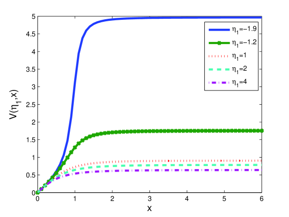
Figure 1: Dependence of the function $V_{1}({\eta_{1}},{\rm x})$ on ${\rm x}\equiv{\rm k_{c}}\xi$ for five different values of $\eta_{1}.$

V-B The Integral Scale

According to Eq. (14), the integral scale in $d=1$ is given by

$$I_{1}({\bm{\theta}}^{\prime})=\xi\frac{\eta_{0}}{G_{\rm x}(0)}=\frac{2\pi\xi}{V_{1}(\eta_{1},{\rm k_{c}}\xi)}.$$ (41)

A distinct feature of the SSRF covariance functions is the nonlinear dependence of the integral scale on the characteristic length $\xi$ for ${\rm k_{c}}\xi\leq 2$. However, if ${\rm k_{c}}\xi\geq 2,$ the integral scale $I_{1}({\bm{\theta}}^{\prime})$ becomes practically independent of the cutoff. Then, $I_{1}({\bm{\theta}}^{\prime})$ is essentially a function of only two variables: the shape parameter ${\eta_{1}}$ and the length $\xi$. The dependence on $\xi$ is linear in this asymptotic regime. More precisely,

$$I_{1}({\eta_{1}},\xi)=\left\{\begin{IEEEeqnarraybox}[]{[}][c]{l^{\prime}s}4\xi\,\beta_{2},&for$|{\eta_1}|<2,$\\ 4\xi,&for${\eta_1}=2$\\ 2\xi\,(\omega_{1}+\omega_{2}),&for${\eta_1}>2.$\end{IEEEeqnarraybox}\right.$$ (42)

While the variance and the integral scale tend to asymptotic values for ${\rm k_{c}}\xi>2,$ this behavior does not extend to the SSRF derivatives, i.e., to the integrals in Eq. (18), which fail to converge with increasing ${\rm k_{c}}$.

V-C Infinite-Band Covariance

The covariance function can be evaluated explicitly for any combination of model parameters by means of the hyperbolic sine and cosine functions, as well as the sine and the cosine integrals. However, the resulting expressions are quite lengthy. Shorter asymptotic expressions are obtained, which are valid for ${\rm k_{c}}\xi>2$. More specifically:

Proposition 2 (FGC-SSRF Covariance)

The Spartan covariance depends linearly on the scale factor $\eta_{0}$. For ${\rm k_{c}}\xi>2$ it becomes a function of the normalized distance $h\equiv|r|/\xi$ and ${\eta_{1}}$ as follows:

$$G_{\rm x}(r)=\eta_{0}\,W_{1}(h,\eta_{1})$$ (43)

where the function $W_{1}(h,\eta_{1})$ is given by the following:

$$W_{1}=\left\{\begin{IEEEeqnarraybox}[]{[}][c]{l^{\prime}s}\,e^{-h\beta_{1}}\left[\frac{\cos(h\beta_{1})}{4\,\beta_{2}}+\frac{\sin(h\beta_{1})}{4\,\beta_{1}}\right],&for$|{\eta_1}|<2,$\\ \frac{(1+h)}{4e^{h}},&for${\eta_1}= 2$\\ \,\frac{1}{\Delta}\,\Big{(}\frac{e^{-h\,\omega_{1}}}{2\omega_{1}}-\frac{e^{-h\,\omega_{2}}}{2\omega_{2}}\Big{)},&for${\eta_1}>2.$\end{IEEEeqnarraybox}\right.$$ (44)

Proof:

The proof is given in the Appendix II. ∎

Corollary 2 (The auto-correlation function)

The auto-correlation function is given by the equation:

$$\rho(r)=\left\{\begin{IEEEeqnarraybox}[]{[}][c]{l^{\prime}s}\,e^{-h\beta_{2}}\left[\cos(h\beta_{1})+\frac{\beta_{2}}{\beta_{1}}\sin(h\beta_{1})\right],&for$|{\eta_1}|<2,$\\ (1+h)\,e^{-h},&for${\eta_1}= 2$\\ \,\frac{\left(\omega_{2}\,e^{-h\omega_{1}}-\omega_{1}\,e^{-h\omega_{2}}\right)}{\omega_{2}-\omega_{1}},&for${\eta_1}>2.$\end{IEEEeqnarraybox}\right.$$ (45)

Proof:

By definition, the autocorrelation function is given by $\rho_{{\rm x}}(r)\doteq G_{\rm x}(r)/\sigma_{\rm x}^{2}$. The Eq. (45) follows from Eqs. (39), (40), and (44). ∎

The autocorrelation function for ${\eta_{1}}=2$ corresponds to the Whittle-Mattérn function, $\rho_{\nu}(r)=\frac{2^{1-\nu}}{\Gamma(\nu)}\,r^{\nu}\,K_{\nu}(r)$ with $\nu=3/2$ [33]. It is interesting to note that the Whittle-Mattérn covariance functions are obtained by solving a stochastic equation with an external white-noise forcing, while the Spartan covariance function is obtained from a Gibbs energy functional. For ${\eta_{1}}>2$, an empirical correlation function is obtained [7]. The correlation function for $|{\eta_{1}}|<2$ provides a class of positive definite functions in $d=1$, which, to our knowledge, is new.

Remark 5

The correlation function obtained for $|{\eta_{1}}|<2$ in Eq. (45) is not merely a superposition of permissible models, since the second term contains a sine function. However, the superposition of the two terms with the precise coefficients ensures the permissibility and the differentiability of the correlation function, in spite of the exponential term.

Plots of the correlation function are shown in Figure (2) for different values of the shape parameter. For ${\eta_{1}}<0$ the correlation function oscillates, and the number of oscillations increases as ${\eta_{1}}\rightarrow-2$. The oscillations disappear for positive values of ${\eta_{1}}$, and a monotonic decline of the correlations due to the exponential terms sets in.

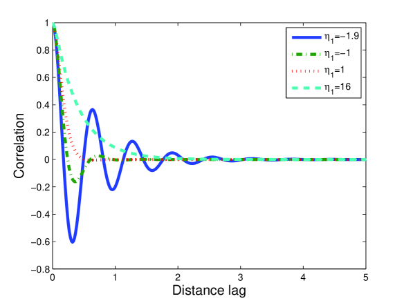
Figure 2: Dependence of the autocorrelation function on distance for different values of the shape parameter ${\eta_{1}}$ with fixed $\xi=0.1.$

VI Covariance of Three-dimensional FGC-SSRF Model

The spectral representation, i.e., Eq. (10), of the isotropic Spartan covariance in $d=3$ is given by

$$G_{\rm x}({\bf r})=\frac{\eta_{0}\xi^{3}\,}{(2\pi)^{3/2}\,r^{1/2}}\,\int\limits_{0}^{\infty}dk\,\frac{k^{3/2}\,J_{1/2}(kr)\,\big{|}\tilde{Q}_{\lambda}(k)\,\big{|}^{2}}{1+\eta_{1}(k\xi)^{2}+(k\xi)^{4}}$$ (46)

Using the identity

$$J_{1/2}(r)=\left(\frac{2}{\pi}\right)^{1/2}\frac{\sin(r)}{r^{1/2}},$$

it follows that

$$G_{\rm x}({\bf r})=\frac{\eta_{0}\xi^{3}\,}{2\pi^{2}\,r}\,\int\limits_{0}^{\infty}dk\,\frac{k\,\sin(kr)\,\big{|}\tilde{Q}_{\lambda}(k)\,\big{|}^{2}}{1+\eta_{1}(k\xi)^{2}+(k\xi)^{4}}.$$

Using the transformation $u=k\xi,$ and the boxcar kernel spectral density, we find

$$G_{\rm x}({\bf r})=\frac{\eta_{0}\xi\,}{2\pi^{2}\,r}\,\int\limits_{0}^{{\rm k_{c}}\xi}du\,\frac{u\,\sin(ru\xi^{-1})}{1+\eta_{1}u^{2}+u^{4}}.$$ (47)

VI-A The Variance

The SSRF variance is calculated based on Eq. (12). We use the dimensionless quantities $\beta_{1}$, $\beta_{2}$, $\omega_{1}$, and $\omega_{2}$ defined in Section (V).

Proposition 3 (FGC-SSRF Variance)

The variance of the Spartan covariance in $d=3$ is given by

$$G_{\rm x}(0)=\frac{\eta_{0}}{4\pi^{2}}V_{3}({\eta_{1}},{\rm k_{c}}\xi)$$ (48)

where

$$V_{3}=\left\{\begin{IEEEeqnarraybox}[]{[}][c]{l^{\prime}s}\frac{1}{4\,\beta_{1}}\ln\left(\frac{{\rm x}^{2}-2\,\beta_{1}{\rm x}+1}{{\rm x}^{2}+2\,\beta_{1}{\rm x}+1}\right)+\\ \frac{1}{2\,\beta_{2}}\sum_{l=-1,1}{\mbox{tan}^{-1}}\left(\frac{{\rm x}+l\,\beta_{1}}{\beta_{2}}\right),&for$|{\eta_1}|<2,$\\ {\mbox{tan}^{-1}}({\rm x})-\frac{{\rm x}}{1+{\rm x}^{2}},&for${\eta_1}=2$\\ \frac{2}{\Delta}\sum_{l=1,2}(-1)^{l}\,\omega_{l}\,{\mbox{tan}^{-1}}\left(\frac{{\rm x}}{\omega_{l}}\right),&for${\eta_1}>2.$\end{IEEEeqnarraybox}\right.$$ (49)

Proof:

The proof is presented in the Appendix III. ∎

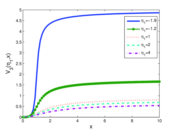
Figure 3: Dependence of the function $V_{3}({\eta_{1}},{\rm x})$ on ${\rm x}\equiv{\rm k_{c}}\xi$ for five different values of $\eta_{1}.$

VI-B The Integral Scale

According to Eq. (14), the integral scale in $d=3$ is given by

$$I_{3}({\bm{\theta}}^{\prime})=\xi\left[\frac{\eta_{0}}{G_{\rm x}(0)}\right]^{1/3}=\xi\,\left[\frac{2\pi^{2}}{V_{3}(\eta_{1},{\rm k_{c}}\xi)}\right]^{1/3}.$$ (50)

As seen in Figure (3), the approach of $V_{3}(\eta_{1},{\rm k_{c}}\xi)$ to the asymptotic limit is slower than in $d=1$. The integral scale $I_{3}({\bm{\theta}}^{\prime})$ becomes practically independent of the cutoff for ${\rm k_{c}}\xi>5$. The asymptotic expressions of the integral scale are:

$$I_{3}({\eta_{1}},\xi)=\left\{\begin{IEEEeqnarraybox}[]{[}][c]{l^{\prime}s}2\,\xi\left(\pi\,\beta_{2}\right)^{1/3}&for$|{\eta_1}|<2,$\\ 2\,\xi\,\pi^{1/3}&for${\eta_1}=2$\\ 2\xi\left[\frac{\pi(\omega_{1}+\omega_{2})}{2}\right]^{1/3},&for${\eta_1}>2.$\end{IEEEeqnarraybox}\right.$$ (51)

VI-C Infinite-Band Covariance

As in $d=1$, the Spartan covariance function can be evaluated explicitly for any ${\bm{\theta}}$ by means of the hyperbolic sine and cosine functions, as well as the sine and the cosine integrals. Here we give the asymptotic (in ${\rm k_{c}}$) expressions:

Proposition 4 (FGC-SSRF Covariance)

The covariance for ${\rm k_{c}}\rightarrow\infty$ is expressed as follows:

$$G_{\rm x}(r)=\frac{\eta_{0}}{2\pi}\,W_{3}(r/\xi,\eta_{1}),$$ (52)

where the function $W_{3}(h,\eta_{1}),\;h=r/\xi$ is given by the following:

$$W_{3}(h,\eta_{1})=\left\{\begin{IEEEeqnarraybox}[]{[}][c]{l^{\prime}s}\>\frac{e^{-h\beta_{1}}}{\Delta}\left[\frac{\sin\left(h\beta_{2}\right)}{h}\right],&for$|{\eta_1}|<2,$\\ \>\frac{1}{4}\,e^{-h},&for${\eta_1}= 2$\\ \>\frac{1}{2\,\Delta}\left(\frac{e^{-h\omega_{1}}-e^{-h\omega_{2}}}{h}\right),&for${\eta_1}>2.$\end{IEEEeqnarraybox}\right.$$ (53)

Proof:

The proof is given in the Appendix IV. ∎

The known exponential covariance is obtained for ${\eta_{1}}=2$, while for $|{\eta_{1}}|<2$ a product of two permissible models, i.e., $\exp(h)$ and $\sin(h)/h$, is obtained. The covariance model obtained for ${\eta_{1}}>2$ is new, at least to our knowledge.

Corollary 3 (The autocorrelation function)

The auto-correlation function is given by the equation:

$$\rho(r)=\left\{\begin{IEEEeqnarraybox}[]{[}][c]{l^{\prime}s}e^{-h\beta_{1}}\left[\frac{\sin\left(h\beta_{2}\right)}{h\beta_{2}}\right],&for$|{\eta_1}|<2,$\\ e^{-h},&for${\eta_1}= 2$\\ \frac{e^{-h\omega_{1}}-e^{-h\omega_{2}}}{h(\omega_{2}-\omega_{1})},&for${\eta_1}>2.$\end{IEEEeqnarraybox}\right.$$ (54)

Proof:

It follows from the definition of the autocorrelation function, as well as Eqs. (48), (49), and (53). ∎

The dependence of the autocorrelation function on distance for various values of ${\eta_{1}}$ is shown in Figure (4). Note that the negative hole for ${\eta_{1}}=-1$ is significantly less pronounced compared to the $d=1$ case.

Remark 6

The Spartan covariances obtained for infinite band in $d=3$ are continuous but non-differentiable, in contrast with the $d=1$ case.

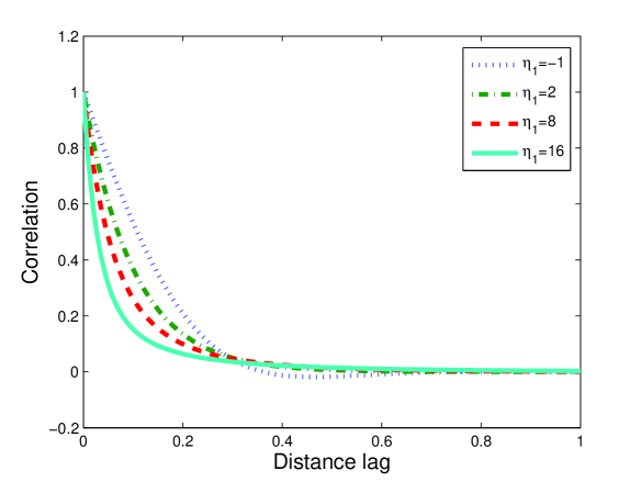
Figure 4: Dependence of the autocorrelation function on distance for different values of the shape parameter ${\eta_{1}}$ with fixed $\xi=0.1$

In $d=2$ the integral of the covariance function can not be evaluated explicitly, even in the infinite band case. However, the covariance functions obtained for $d=3$ are also permissible $d=1,2$ [1, pp. 30-31]. Of course, they are not derived from the FGC-SSRF model in $d<3$.

VII Discussion and Conclusions

We showed that FGC Spartan Spatial Random Fields are analytic in any dimension, provided that the covariance spectral density is band-limited. We calculated the variance and the integral scale of the FGC-SSRF covariance functions in one and three dimensions. We also obtained explicit expressions for the covariance function at the asymptotic limit (i.e., the infinite-band limit). Depending on the value of the shape parameter ${\eta_{1}}$, the resulting expressions were shown to recover known models or to yield new covariance functions.

Explicit expressions for the covariance functions in $d=1,3$ are also possible in the pre-asymptotic limit. However, they are not given here since they are very lengthy, and in practice it may be preferable to integrate Eq. (10) numerically. It was also shown that the asymptotic expressions are quite accurate for the covariance function (but not for its derivatives) when the product ${\rm k_{c}}\xi$ exceeds a finite, dimensionality-dependent threshold. This result has practical applications in SSRF parameter inference, since the procedure used involves matching ensemble constraints, which are expressed in terms of the covariance function, with respective sample constraints [18, 35].

Explicit expressions for the covariance function were not found in $d=2$, where the presence of $J_{0}(kr)$ prohibits closed form integration in Eq. (10). Explicit expressions for the variance are given in [22], and for the integral scale in [35].

The FGC-SSRF covariance functions permit a continuous transition between smooth (analytic) and rough (non-analytic) states, by controlling the spectral band cutoff ${\rm k_{c}}$. This property is shared by the Whittle-Matérn covariance functions.

Besides providing new covariance functions, the SSRF idea focuses on representing spatial structure using energy functionals with clear physical interpretation. These lead to new possibilities for parameter inference and spatial interpolation in geostatistical applications, which are the target of continuing investigations [18, 23, 35, 37].

Appendix A Proof of Proposition 1

Proof:

We calculate the integrals required for evaluating the variance of the 1D SSRF.

Step (i): $|\eta_{1}|<2.$ We define the characteristic polynomial $\Pi({\rm x})\doteq{\rm x}^{4}+{\eta_{1}}{\rm x}^{2}+1$. We expand $\Pi(x)$ as follows:

$$\Pi({\rm x})=({\rm x}^{2}+2\beta_{1}{\rm x}+1)({\rm x}^{2}-2\beta_{1}{\rm x}+1),$$

where $\beta_{1}$ is given by Eq. (37).

Using partial fraction expansion we obtain

$$\frac{1}{\Pi({\rm x})}=\frac{1}{8\beta_{1}}\left(\frac{2{\rm x}+2\beta_{1}}{{\rm x}^{2}+2\beta_{1}{\rm x}+1}-\frac{2{\rm x}-2\beta_{1}}{{\rm x}^{2}-2\beta_{1}{\rm x}+1}\right)$$

$$+\frac{1}{2+{\eta_{1}}}\left[\frac{1}{1+(\frac{{\rm x}+\beta_{1}}{\beta_{2}})^{2}}+\frac{1}{1+(\frac{{\rm x}+\beta_{1}}{\beta_{2}})^{2}}\right],\\$$ (55)

where $\beta_{2}$ is given by Eq. (38). Then, by direct integration the following is obtained:

$$\int d{{\rm x}}\,\frac{1}{\Pi({\rm x})}=\frac{1}{8\beta_{1}}\log\left(\frac{{\rm x}^{2}+2\beta_{1}{\rm x}+1}{{\rm x}^{2}-2\beta_{1}{\rm x}+1}\right)$$

$$+\frac{1}{4\beta_{2}}\left\{{\mbox{tan}^{-1}}\left(\frac{{\rm x}+\beta_{1}}{\beta_{2}}\right)+{\mbox{tan}^{-1}}\left(\frac{{\rm x}-\beta_{1}}{\beta_{2}}\right)\right\}.\\$$

Step (ii): $\eta_{1}=2.$ In this case one obtains:

$$\frac{1}{\Pi({\rm x})} = \frac{1}{2}\;\frac{1+{\rm x}^{2}}{(1+{{\rm x}}^{2})^{2}}+\frac{1}{2}\;\frac{1-{\rm x}^{2}}{(1+{{\rm x}}^{2})^{2}}$$ (56)

$$= \frac{1}{2(1+{{\rm x}}^{2})}+\frac{1-{\rm x}^{2}}{2(1+{{\rm x}}^{2})^{2}}.$$

It follows that

$$\int d{{\rm x}}\,\frac{1}{\Pi({\rm x})}=\frac{{\mbox{tan}^{-1}}({\rm x})}{2}+\frac{{\rm x}}{2(1+{\rm x}^{2})}.$$

Step (iii): $\eta_{1}>2.$ In this case $\Pi({\rm x})$ is expressed as follows:

$$\Pi({\rm x})=\big{(}{\rm x}^{2}+\omega_{1}^{2}\big{)}\big{(}{\rm x}^{2}+\omega_{2}^{2}\big{)},$$

where $\omega_{1,2}$ are given by Eq. (38). We find

$$\int d{{\rm x}}\frac{1}{\Pi({\rm x})}=\frac{1}{\Delta}\int d{\rm x}\left(\frac{1}{{\rm x}^{2}+\omega_{1}^{2}}-\frac{1}{{\rm x}^{2}+\omega_{2}^{2}}\right)$$

$$=\frac{1}{\Delta}\left[\frac{1}{\omega_{1}}{\mbox{tan}^{-1}}\left(\frac{{\rm x}}{\omega_{1}}\right)-\frac{1}{\omega_{2}}{\mbox{tan}^{-1}}\left(\frac{{\rm x}}{\omega_{2}}\right)\right].$$

∎

==========================================================

Appendix B Proof of Proposition 2

Proof:

Let us define the normalized distance $h=|r|/\xi$. We evaluate the integrals using integration in the complex plane. More specifically, based on the residue theorem and Jordan’s lemma [8, pp. 358-370], we obtain

$$\int\limits_{0}^{\infty}d{\rm x}\frac{\cos(h{\rm x})}{\Pi({\rm x})}=\Re\left\{\pi\jmath\,\sum\mbox{Res}^{+}\left[\frac{\exp(\jmath hz)}{\Pi(z)}\right]\right\},$$ (57)

where $\sum\mbox{Res}^{+}\left[Q(z)\right]$ denotes the sum of the residues of the function $Q(z)$ in the upper half plane, and $\Re[A(z)]$ denotes the real part of the complex function $A(z).$

Step (i): $|\eta_{1}|<2.$

Since $\Pi(z)=\left(z^{2}+2\beta_{1}z+1\right)\left(z^{2}-2\beta_{1}z+1\right)$ the imaginary poles in the upper half plane are $z_{\pm}=\pm\beta_{1}+{\jmath}\;\beta_{2}.$ Thus, we obtain

$$\sum_{z=z_{\pm}}\mbox{Res}^{+}\left[\frac{\exp(\jmath\,hz)}{\Pi(z)}\right]=\frac{{\jmath}}{2\beta_{2}}$$

$$\!\!\!\left[\frac{e^{-h\left(\beta_{2}+{\jmath}\,\beta_{1}\right)}}{{\eta_{1}}-2+{\jmath}\,\Delta}+\frac{e^{-h\left(\beta_{2}-{\jmath}\,\beta_{1}\right)}}{{\eta_{1}}-2-{\jmath}\,\Delta}\right]$$

and

$$\Re\left\{\jmath\sum_{z=z_{\pm}}\mbox{Res}^{+}\left[\frac{\exp(\jmath\,hz)}{\Pi(z)}\right]\right\}=\frac{e^{-h\beta_{2}}}{(4{\eta_{1}}-8)\beta_{2}}$$

$$\big{[}\,({\eta_{1}}-2)\cos\left(h\beta_{1}\right)-\Delta\sin\left(h\beta_{1}\right)\,\big{]}.$$

Step (ii): ${\eta_{1}}=2$.

Since $\Pi(z)=(1+z^{2})^{2}$, in the upper-half plane there is a double imaginary pole, $z_{+}=\jmath$. Hence,

$$\int\limits_{0}^{\infty}d{{\rm x}}\frac{\cos({\rm x}h)}{(1+{{\rm x}}^{2})^{2}} = \Re\left\{\pi{\jmath}\Big{(}-{\jmath}\;\frac{1+h}{4e^{h}}\Big{)}\right\}$$

$$= \frac{\pi(1+h)}{4e^{h}}.$$

Step (iii): $\eta_{1}>2.$ Using the variables $\omega_{j},$ recall from Appendix I that

$$\frac{1}{\Pi(z)}=\frac{1}{\Delta}\left(\frac{1}{z^{2}+\omega_{1}^{2}}-\frac{1}{z^{2}+\omega_{2}^{2}}\right).$$

Thus

$$\int\limits_{0}^{\infty}d{{\rm x}}\frac{\cos({\rm x}h)}{\Pi({\rm x})} = \frac{1}{\Delta}\Re\left\{\pi\jmath\,\Big{(}\frac{e^{-h\omega_{1}}}{2{\jmath}\;\omega_{1}}-\frac{e^{-h\omega_{2}}}{2{\jmath}\;\omega_{2}}\Big{)}\right\}$$

$$= \frac{\pi}{\Delta}\Big{(}\frac{e^{-h\omega_{1}}}{2\omega_{1}}-\frac{e^{-h\omega_{2}}}{2\omega_{2}}\Big{)}.$$

∎

Appendix C Proof of Proposition 3

Proof:

We calculate the integrals required for evaluating the variance of the 3D SSRF.

Step (i): $|\eta_{1}|<2.$

Using the partial fraction expansion we obtain

$$\frac{{\rm x}^{2}}{\Pi({\rm x})}=\frac{1}{8\beta_{1}}\left(\frac{2{\rm x}-2\beta_{1}}{{\rm x}^{2}-2\beta_{1}{\rm x}+1}-\frac{2{\rm x}+2\beta_{1}}{{\rm x}^{2}+2\beta_{1}{\rm x}+1}\right)$$

$$+\frac{1}{2}\;\frac{{\rm x}^{2}+1}{({\rm x}^{2}+2\beta_{1}{\rm x}+1)({\rm x}^{2}-2\beta_{1}{\rm x}+1)}.$$

By direct integration we obtain

$$\int d{{\rm x}}\,\frac{{\rm x}^{2}}{\Pi({\rm x})}=\frac{1}{8\beta_{1}}\log\left(\frac{{\rm x}^{2}-2\beta_{1}{\rm x}+1}{{\rm x}^{2}+2\beta_{1}{\rm x}+1}\right)$$

$$+\frac{1}{4\beta_{2}}\left\{{\mbox{tan}^{-1}}\left(\frac{{\rm x}+\beta_{1}}{\beta_{2}}\right)+{\mbox{tan}^{-1}}\left(\frac{{\rm x}-\beta_{1}}{\beta_{2}}\right)\right\}.\\$$

Step (ii): $\eta_{1}=2.$ In this case the partial fraction expansion becomes

$$\frac{{\rm x}^{2}}{\Pi({\rm x})}=\frac{1}{2(1+{{\rm x}}^{2})}-\frac{1-{\rm x}^{2}}{2(1+{{\rm x}}^{2})^{2}}.$$

It follows that

$$\int d{{\rm x}}\,\frac{{\rm x}^{2}}{\Pi({\rm x})} = \frac{1}{2}\left[\,{\mbox{tan}^{-1}}({\rm x})-\frac{{\rm x}}{1+{\rm x}^{2}}\right].$$

Step (iii): $\eta_{1}>2.$

In this case

$$\Pi({\rm x})=\left({\rm x}^{2}+\omega_{1}^{2}\right)\left({\rm x}^{2}+\omega_{2}^{2}\right),$$

and

$$\frac{{\rm x}^{2}}{\Pi({\rm x})}=\frac{1}{\Delta}\left(\frac{\omega_{2}^{2}}{{\rm x}^{2}+\omega_{2}^{2}}-\frac{\omega_{1}^{2}}{{\rm x}^{2}+\omega_{1}^{2}}\right).$$

It follows that

$$\int d{{\rm x}}\,\frac{{\rm x}^{2}}{\Pi({\rm x})}=\frac{1}{\Delta}\left[\omega_{2}\,{\mbox{tan}^{-1}}\left(\frac{{\rm x}}{\omega_{2}}\right)-\omega_{1}\,{\mbox{tan}^{-1}}\left(\frac{{\rm x}}{\omega_{1}}\right)\right].$$

∎

Appendix D Proof of Proposition 4

Proof:

We follow the same procedure for integrating the covariance spectral density as in the Appendix II. In $d=3$ the respective integral is given by:

$$\int\limits_{0}^{\infty}d{\rm x}\frac{{\rm x}\sin(h\,{\rm x})}{\Pi({\rm x})}=\Im\left\{\pi\jmath\sum\mbox{Res}^{-}\left[\frac{z\;e^{-\jmath\,hz}}{\Pi(z)}\right]\right\},$$

where $\sum\mbox{Res}^{-}\left[Q(z)\right]$ denotes the sum of the residues of the function $Q(z)$ in the lower half plane, and $\Im[A(z)]$ denotes the imaginary part of the complex function $A(z).$

Step (i): $|\eta_{1}|<2.$

The imaginary poles in the lower half plane are

$$z_{\pm}=\pm\beta_{1}-{\jmath}\;\beta_{2}.$$

We have

$$\sum_{z=z_{\pm}}\mbox{Res}^{-}\left[\frac{z\;e^{-\jmath\,hz}}{\Pi(z)}\right]=\frac{{\jmath}}{2\beta_{2}}$$

$$\left\{\frac{\beta_{1}\;e^{-h\,\left(\beta_{2}+{\jmath}\beta_{1}\right)}}{2-{\eta_{1}}}-\frac{\beta_{1}\;e^{-h\,\left(\beta_{2}-{\jmath}\beta_{1}\right)}}{2-{\eta_{1}}}\right\}$$

$$= \frac{1}{\Delta}\;\sin\left(h\,\beta_{1}\right)\;e^{-h\,\beta_{2}}.$$

Thus,

$$\int\limits_{0}^{\infty}d{\rm x}\frac{{\rm x}\sin(h\,{\rm x})}{\Pi({\rm x})}=\frac{\pi}{\Delta}\;\sin\left(h\,\beta_{1}\right)\;e^{-h\,\beta_{2}}.\\$$ (58)

Step (ii): $\eta_{1}=2.$

$$\int\limits_{0}^{\infty}d{\rm x}\;\frac{{\rm x}\sin({\rm x}\,h)}{\Pi({\rm x})}=\int\limits_{0}^{\infty}d{\rm x}\;\frac{{\rm x}\sin({\rm x}\,h)}{({\rm x}^{2}+1)^{2}}=\frac{\pi\,h\,e^{-h}}{4}.$$

Step (iii): $\eta_{1}>2.$ Using $\Pi(z)=\left(z^{2}+\omega_{2}^{2}\right)\left(z^{2}+\omega_{1}^{2}\right)$, we obtain

$$\frac{z\sin(z\,h)}{\Pi(z)}=\frac{1}{\Delta}\left\{\frac{z\sin(z\,h)}{z^{2}+\omega_{1}^{2}}-\frac{z\sin(z\,h)}{z^{2}+\omega_{2}^{2}}\right\}.$$

The poles in the lower half plane are $z_{+}=-{\jmath}\,\omega_{2}$ and $z_{-}=-{\jmath}\,\omega_{1}.$ It then follows that:

$$\int\limits_{0}^{\infty}d{\rm x}\;\frac{{\rm x}\sin({\rm x}\,h)}{\Pi({\rm x})}=\frac{\pi}{\Delta}\;\Im\left\{\jmath\;\mbox{Res}^{-}\left[\frac{z\;e^{-\jmath\,hz}}{z^{2}+\omega_{1}^{2}}\right]_{z_{-}}\right.$$

$$-\left.\jmath\;\mbox{Res}^{-}\left[\frac{z\;e^{-\jmath\,hz}}{z^{2}+\omega_{2}^{2}}\right]_{z_{+}}\right\}=\frac{\pi}{2\Delta}\left(e^{-h\,\omega_{1}}-e^{-h\,\omega_{2}}\right).$$

∎

References

- [1] P. Abrahamsen, “A Review of Gaussian Random Fields and Correlation Functions,” Norwegian Computing Center, Box 114, Blindern, N-0314, Oslo, Norway 2nd ed., Tech. Rep. 917, 1997.
- [2] R. J. Adler and J. E. Taylor, Random Fields and Geometry. February 21, 2006. [Online]. Available: http://iew3.technion.ac.il/ radler/publications.html
- [3] J. Ruiz-Alzola et al., “Geostatistical Medical Image Registration” in Proc. of 6th Intern. Conf. Medical Image Comput. Computer-Assisted Intervention (MICCAI’03), 2003, pp. 894-201.
- [4] M. Armstrong, Basic Linear Geostatistics. Berlin: Springer, 1998.
- [5] J. Besag and C. Kooperberg, “On conditional and intrinsic autoregressions,” Biometrika, vol. 82, pp. 733-746, Dec. 1995.
- [6] S. Bochner, Lectures on Fourier Integrals. Princeton, NJ: Princeton University Press, 1959.
- [7] C. E. Buell, “Correlation functions for wind and geopotential on isobaric surfaces,” J. Appl. Meteor., Vol. 11, pp. 51-59, Feb. 1972.
- [8] F. W. Jr. Byron and R. W. Fuller, Mathematics of Classical and Quantum Physics. NY: Dover, 1992.
- [9] J. Cao and K. J. Worsley, “Applications of random fields in human brain mapping” in Spatial Statistics: Methodological Aspects and Applications, Springer Lecture Notes in Statistics, M. Moore (Ed.), Vol. 159, pp. 169-182, 2001.
- [10] G. Christakos, Random Field Models in Earth Sciences. San Diego, CA: Academic Press, 1992.
- [11] G. Christakos and D. T. Hristopulos, Spatiotemporal Environmental Health Modelling. Boston: Kluwer, 1998.
- [12] N. Cressie, Statistics for Spatial Data. NY: Wiley, 1993.
- [13] M. Galetakis and D. T. Hristopulos, “Prediction of long-term quality fluctuations in the South Field lignite mine of West Macedonia,” in Proc. AMIREG, 2004, pp. 133-138. Athens: Heliotopos Conferences.
- [14] L. W. Gelhar, Stochastic Subsurface Hydrology. Englewood Cliffs, NJ:Prentice Hall, 1993.
- [15] P. Goovaerts, Geostatistics for Natural Resources Evaluation. New York: Oxford University Press, 1997.
- [16] M. E. Hohn, Geostatistics and Petroleum Geology. Dordrecht: Kluwer, 1999.
- [17] D. T. Hristopulos, “New anisotropic covariance models and estimation of anisotropic parameters based on the covariance tensor identity,” Stoch. Env. Res. Risk A., Vol. 16, pp. 43-62, Feb. 2002.
- [18] D. T. Hristopulos, “Spartan Gibbs random field models for geostatistical applications,” SIAM J. Sci. Comput., Vol. 24, No. 6, pp. 2125-2162, 2003.
- [19] D. T. Hristopulos, “Simulations of Spartan random fields,” in Proc. ICCMSE, 2003, pp. 242-247. London, UK: World Scientific.
- [20] D. T. Hristopulos, “Anisotropic Spartan random field models for geostatistical analysis,” in Proc. International Conference on Advances in Mineral Resources Management and Environmental Geotechnology. Athens: Heliotopos Conferences, 2004, pp. 127-132.
- [21] D. T. Hristopulos, “Identification of spatial anisotropy by means of the covariance tensor identity,” in Mapping Radioactivity in the Environment: Spatial Interpolation Comparison 2005, G. Dubois and S. Galmarini, Eds. Luxembourg: Office for Official Publications of the European Communities. [Online]. Available: www.ai-geostats.org
- [22] D. T. Hristopulos, “Non-constrained simulations of Gaussian Spartan random fields in two dimensions,” Math. Comput. Model., to be published.
- [23] D. T. Hristopulos, “Spatial random field models inspired from statistical physics with applications in the geosciences,” Physica A, Vol. 365, No. 1, pp. 211-216, 2006.
- [24] A. G. Journel and C. J. Huigbregts, Mining Geostatistics. London: Academic Press, 1978.
- [25] M. Kanevsky, and M. Maignan, Analysis and Modelling of Spatial Environmental Data. New York: M. Dekker, 2004.
- [26] P. K. Kitanidis, Introduction to Geostatistics: Applications to Hydrogeology. Cambridge: Cambridge University Press, 1997.
- [27] C. Lantuejoul, Geostatistical Simulation: Models and Algorithms. Berlin: Springer, 2001.
- [28] A. Leow et al., “Brain structural mapping using a novel hybrid implicit/explicit framework based on the level-set method,” NeuroImage, Vol. 24, No. 3, pp. 910 927, 2004.
- [29] G. Matheron, “The intrinsic random functions and their applications,” Adv. Appl. Probab., Vol. 5, No. 2, pp. 439-468, 1973.
- [30] Y. Rubin , Applied Stochastic Hydrogeology. New York: Oxford University Press, 2003.
- [31] H. Rue, “Fast sampling of Gaussian Markov random fields,” J. Roy. Stat. Soc. B, Vol. 63, No. 2, pp. 325-338, 2001.
- [32] H. Rue and H. Tjelmeland, “Fitting Gaussian Markov random fields to Gaussian fields,” Scand. J. Stat., Vol. 29, pp. 31-49, Mar. 2002.
- [33] N. V. Semenovs’ka and M. I. Yadrenko, “Explicit extrapolation formulas for correlation models of homogeneous isotropic random fields,” Theor. Probab. Math. Statist., Vol. 69, pp. 175-185, 2004.
- [34] D.O. Siegmund and K.J. Worsley, “Testing for a signal with unknown location and scale in a stationary Gaussian random field,” Ann. Statist., Vol. 23, pp. 608 639, 1995.
- [35] S. Elogne and D. T. Hristopulos (2006, March). On the inference of Spartan spatial random field models for geostatistical applications. [Online]. Available: wwww.arxiv-math/0603430.
- [36] R. L. Smith, “Spatial statistics in environmental science,” in Nonlinear and Nonstationary Signal Processing, W. J. Fitzgerald, R. L. Smith, A. T. Walden and P. C. Young, Eds. Cambridge: Cambridge University Press, 2000, pp. 152-183.
- [37] M. Varouchakis, and D. T. Hristopulos, “Mapping of soil contaminants using spatial Spartan random fields: a comparative study,” in Proc. Intern. Workshop in Geoenvironment and Geotechnics, Z. Agioutantis, Ed. Athens: Heliotopos Conferences, 2005, pp. 235-240.
- [38] H. Wackernagel, Multivariate Geostatistics. Berlin: Springer, 2003.
- [39] E. T. Whittaker and G N. Watson, A Course of Modern Analysis, 4th ed., New York, Cambridge University Press, 1992.
- [40] R. Wilson and C.T. Li, “A class of discrete multiresolution random fields and its application to image segmentation,” IEEE T. Pattern Anal., Vol. 25, pp. 42-56, Jan. 2002.
- [41] G. Winkler, Image Analysis, Random Fields and Dynamic Monte Carlo Methods. Berlin: Springer, 1995.
- [42] A. M. Yaglom, Correlation Theory of Stationary and Related Random Functions I: Basic Results. New York: Springer, 1987.