Parallel vs. Sequential Belief Propagation Decoding of LDPC Codes over $GF(q)$
and Markov Sources

Abstract

A sequential updating scheme (SUS) for belief propagation (BP) decoding of LDPC codes over Galois fields, $GF(q)$, and correlated Markov sources is proposed, and compared with the standard parallel updating scheme (PUS). A thorough experimental study of various transmission settings indicates that the convergence rate, in iterations, of the BP algorithm (and subsequently its complexity) for the SUS is about one half of that for the PUS, independent of the finite field size $q$. Moreover, this $1/2$ factor appears regardless of the correlations of the source and the channel’s noise model, while the error correction performance remains unchanged. These results may imply on the ’universality’ of the one half convergence speed-up of SUS decoding.

Index Terms: LDPC codes over $GF(q)$, Markov sources, belief propagation, joint source-channel decoding, sequential updating.

1 Introduction

Low density parity check (LDPC) codes, first invented by Gallager in 1962 [1] and long afterwards rediscovered in the seminal work of MacKay and Neal (MN, [2]), play a fundamental role in modern communications, primarily due to their near-Shannon limit performance. An almost optimal, yet tractable decoding [2] of this class of codes is empowered by the renowned probabilistic message passing algorithm of belief propagation (BP, [3]).

It was also shown [4] that the remarkable error performance of Gallager’s binary LDPC codes can be significantly enhanced even further by a generalization to higher finite Galois fields, $GF(q)$ with $\mathbb{Z}\ni q>2$. This behavior can be rationalized by the fact that the graphical representation of such codes has less edges and subsequently relatively longer loops.

As BP is an iterative algorithm, its convergence rate is also a crucial benchmark in its implementation as a decoder. In principle, as the communication channel becomes noisier the decoding time increases, since the latter is dictated by the total number of BP message passing iterations required for convergence [5]. Furthermore, this number of iterations tends to diverge when approaching the channel’s capacity [6].

Kfir and Kanter [7] were the first to introduce a serialization method which was shown, by providing convincing empirical results, to yield half the decoding time and complexity w.r.t. parallel (flooding) scheduling, while the error performance does not deteriorate. Following, several sequential (serial) BP message passing schedules were recently introduced (e.g. , [8] and references therein). It was shown, either via semi-analytical methods [8, 9, 10] or by simulations [11], that such sequential schedules converge faster than the standard parallel schedule.

Despite the aforementioned contributions addressing binary LDPC codes, there has been no examination of the effect of serialization on LDPC codes over $GF(q)$. In this letter, based on a thorough experimental study of a $GF(q)$ extension of the serialization scheme originally proposed by Kfir and Kanter [7], we find that not only sequential decoding over $GF(q)$ accelerates BP convergence w.r.t. standard flooding, but interestingly the same $1/2$ convergence ratio arises. The error correction performance is roughly preserved.

In addition, the convergence of sequential decoding is investigated for correlated information sources, an issue yet to be discussed in the literature, addressing only independent and identically distributed (i.i.d.) sources. Here, the source is modelled by a Markov process, while a method of dynamical block priors[12] is incorporated within the BP decoding in order to exploit the prior knowledge on the source statistics and form a joint source-channel decoding scheme (the move to $GF(q)$ enables the treatment of Markov sequences with a richer alphabet). Again, the same factor $1/2$ emerges in this case too, accelerating the convergence of sequential BP decoding substantially. These results are corroborated via simulations for the binary symmetric channel (BSC), binary erasure channel (BEC) and the binary-input additive white Gaussian noise (BI-AWGN) channel.

To sum up, the one half factor is found to be robust to the following extensions: 1) extension of binary sources, $q=2$, to higher finite field, $q>2$, 2) extension of BP for i.i.d. sources to the case of BP with dynamical priors used for joint source-channel decoding, and 3) extension of the BSC case to other popular channel models. This extension may imply on the ’universality’ of the $1/2$ convergence speed-up ratio of sequential BP decoding.

2 Sequential and Parallel Joint Source-Channel Decoding

Consider a MN code with two sparse matrices known both to the transmitter and the receiver, ${\bf A}(M\times N)$ and ${\bf B}(M\times M)$, where the indices $N,M$ are the source block length and the transmitted block length, respectively. All non-zero elements in ${\bf A}$ and ${\bf B}$ are taken randomly from $\{1,2,\ldots,q-1\}\in GF(q)$, and $B$ must be invertible.

A proper construction of these matrices is crucial in order to ensure capacity-achieving performance. In this work we follow the Kanter-Saad (KS, [6]) construction, which yields very sparse, simple to construct matrices, known to perform very close to the bound.

Thus encoding a source vector ${\bf s}$ into a codeword ${\bf t}$, with rate $R=N/M$, is performed by

$${\bf t}={\bf B}^{-1}{\bf A}{\bf s}\mod q,$$ (1)

where ${\bf t}$ is converted to binary representation and transmitted over the channel. During transmission, the coded information ${\bf t}$ is corrupted by a noise vector ${\bf n}$, resulting in the received vector ${\bf r}={\bf t}+{\bf n}\mod 2$.

Upon receipt, the decoder reconverts ${\bf r}$ back to the original field and computes the syndrome ${\bf z}={\bf B}{\bf r}$, which can be reformulated as

$${\bf z}={\bf B}({\bf B}^{-1}{\bf A}{\bf s}+{\bf n})=[{\bf A}{\bf B}]{\bf x}\triangleq{\bf H}{\bf x}\mod q,$$ (2)

where the operator $[\cdot]$ denotes appending of matrices, and vector ${\bf x}$ is a concatenation of ${\bf s}$ and ${\bf n}$. The decoding problem is solved efficiently using the BP algorithm, as follows.

The non-zero elements in a row $i$ of the matrix ${\bf H}$ represent the bits of vector ${\bf x}$ participating in the corresponding check, $z_{i}$. The non-zero elements in column $j$ represent the checks in which the $j$’th bit participates. For each non-zero element in H, the algorithm calculates different types of coefficients.

The coefficient $q^{a}_{ij}$ stands for the probability that the bit $x_{j}$ is $a\in GF(q)$, taking into account the information of all checks in which it participates, except for the $i$’th check. The coefficient $r_{ij}^{a}$ indicates the probability that the bit $x_{j}$ is $a$, taking into account the information of all bits participating in the $i$’th check, except for the $j$’th bit.

The parallel updating scheme (PUS) consists of alternating horizontal and vertical passes over the ${\bf H}$ matrix. Each pair of horizontal and vertical passes is defined as an iteration. In the horizontal pass, all the $r_{ij}^{a}$ coefficients are updated, row after row, by

$$r^{a}_{ij}=\sum_{(all\,configurations\,with\,x_{j}=a,\,satisfing\,z_{i})}\prod_{j^{\prime}\neq j}q_{ij^{\prime}}^{x_{j^{\prime}}},$$ (3)

where it is clear that the multiplication is performed only over the non-zero elements of the matrix ${\bf H}$.

In the vertical pass, all $q^{a}_{ij}$ are computed, column by column, using the updated values of $r^{a}_{ij}$

$$q_{ij}^{a}=\alpha_{ij}p_{j}^{a}\prod_{i^{\prime}\neq i}r_{i^{\prime}j}^{a},$$ (4)

where $\alpha_{ij}$ is a normalization factor such that $\sum_{a=1}^{q}q_{ij}^{a}=1$, and $p_{j}^{a}$ represents the prior knowledge about bit $j$ being in state $a$. Now the pseudo-posterior probability can be computed by

$$Q_{j}^{a}=\alpha_{j}p_{j}^{a}\prod_{i}r_{ij}^{a}.$$ (5)

Again, $\alpha_{j}$ is a normalization constant satisfying $\sum_{a=1}^{q}Q^{a}_{j}=1$, and $i$ runs only over non-zero elements of ${\bf H}$. Each iteration ends by generating the estimates $\hat{{\bf x}}$ by clipping the $Q_{j}$’s.

At the end of each iteration a convergence test, checking if $\hat{{\bf x}}$ solves ${\bf H}\hat{{\bf x}}={\bf z}$, is performed. If some of the $M$ equations are violated, the algorithm turns to the next iteration until a pre-defined maximal number of iterations is reached with no convergence. Note that there is no inter-iteration information exchange between the bits: all $r_{ij}^{a}$ values are updated using the previous iteration data.

In the proposed sequential updating scheme (SUS), we perform the horizontal and vertical passes separately for each bit in ${\bf x}$. A single sequential iteration for the bit $x_{j}$ consists of the following steps:

1. For a given $j$ all $r_{ij}^{a}$ are updated. More precisely, for all non-zero elements in column $j$ of ${\bf H}$, use Eq. (3) for updating $r_{ij}$. Note that this is only a partial horizontal pass, since only $r_{ij}^{a}$’s belonging to a specific column are updated.

2. After all $r_{ij}^{a}$’s belonging to a column $j$ are updated, a vertical pass as defined in Eq. (4) is performed over column $j$. Again, this is a partial vertical pass, referring only to one column.

3. Steps 1-2 are repeated for the next column, until all columns in ${\bf H}$ are updated.

4. Finally, the pseudo-posterior probability value $Q_{j}$, is computed by Eq. (5).

After all variable nodes are updated, the algorithm continues as for the parallel scheme: clipping, checking the validity of the $M$ equations and proceeding to the next iteration.

As for the priors, side information on the Markovian nature of the source is dynamically incorporated within the decoding process. During the vertical pass, a prior knowledge is assigned to each decoded symbol according to the assumed statistics (evidently, for the i.i.d. case this would simply be $\Pr(s=a)=1/q$ for all the source symbols.)

The key here is that one can re-estimate and re-assign these priors after every iteration. Consider, for instance, three successive $GF(q)$ source symbols, $s_{i-1}=a,s_{i}=b$ and $s_{i+1}=c$. The prior $Pr(s_{i}=b)$ can be achieved by the formula

$$P_{i}^{b}=\sum_{a,c=0}^{q-1}Q_{i-1}^{a}\cdot M_{ab}\cdot M_{bc}\cdot Q_{i+1}^{c},$$ (6)

where ${\bf M}$ is the measured Markov transition matrix. The complexity of this updating rule is $\mathcal{O}(q^{2})$. Reducing it to $\mathcal{O}(q)$, the Eq. (6) can be rewritten as

$$P_{i}^{b}=\sum_{a=0}^{q-1}Q_{i-1}^{a}\cdot M_{ab}\sum_{c=0}^{q-1}M_{bc}\cdot Q_{i+1}^{c}.$$ (7)

As for the noise bit ($j>N$), the coefficient is initialized, for instance in the BSC case, to be $Q_{j}^{a}=f^{L}(1-f)^{\log_{2}{q}-L}$, where $L$ is the number of $1$’s in the bits presentation of the symbol $a$. Then we set $q_{ij}^{a}=Q_{j}^{a}$ for all non-zero elements in the $j$’th column.

Note that the complexity per single iteration is almost the same for both updating methods. Hence, the gain in iterations actually represents the gain in decoding complexity.

3 Results

In order to evaluate the nature of BP convergence, our experimental study consists of decoding various LDPC codes over $GF(q)$ for both correlated and uncorrelated information sources. We perform simulations of decoding over the popular BSC, BEC and the BI-AWGN channel, using various noise levels (i.e. , flip rates, erasure rates and signal to noise ratios, repectively). The noise levels are chosen to be close to the noise threshold of the code in order to get substantial convergence time. The KS code construction is used with $N=10000/\log_{2}{q}$ source symbols.

Table 1 compares the average convergence and error rates for the SUS and PUS. A LDPC code of rate $1/3$ is used, although similar results are obtained also for other code rates, and the statistics is collected over at least 6000 different samples. The correlated sources are modeled by adopting typical 2-state (2S) and 4-state (4S) Markov processes with entropy 1/2. A convergence speed-up factor of $1/2$, in favor of SUS, appears. This factor is consistent regardless of the $GF$ order and the source correlation. The standard deviation is relatively small for all cases. Note that this speed-up does not deteriorate the code’s error performance. As our statistics is collected over $\sim 6000$ samples of block size $10^{4}$, we do not report the exact value for bit error rate (BER) $P_{b}\leq 10^{-6}$.

Fig. 1 presents the ratio between PUS and SUS in the percentage of corrected bits per iteration as a function of the total percentage of correct bits. To be more precise, the correction gain, i.e. the difference between the percentage (w.r.t. the block’s size) of bits corrected in the following iteration and in the current iteration, $\Delta{P}$, is calculated and the average ratio for SUS and PUS

$$\frac{<\Delta{P_{PUS}>}}{<\Delta{P_{SUS}}>},$$ (8)

is drawn as a function of the percentage of the current correct bits $P$.

It can be easily seen that the one half ratio is preserved through all the process of decoding, regardless of the decoding dynamics and the system’s state. These results are obtained for transmitting a 2S-Markov source via a BSC ($f=0.23$) using a $GF(8)$ rate $1/3$ LDPC code, although similar results are found for the BEC and BI-AWGN channel cases, using all other investigated transmission settings, as listed in Table 1.Notice that the last point in Fig. 1, indicating the end of the decoding process, is higher (around $0.7$) since at this final stage the error correction improvement by SUS can not be twice that achieved for PUS.

Table 1: SUS vs. PUS: convergence and error rates

Channel	GF	Source	Noise	$\begin{array}[]{c}\mathbf{<t_{SUS}>}\\ (iterations)\end{array}$	$\begin{array}[]{c}\mathbf{<t_{PUS}>}\\ (iterations)\end{array}$	$\mathbf{\frac{<t_{SUS}>}{<t_{PUS}>}}$	$\mathbf{<\frac{t_{SUS}}{t_{PUS}}>}$	STDEV($\mathbf{\frac{t_{SUS}}{t_{PUS}}}$)	$\begin{array}[]{c}\mathbf{BER}(\times 10^{-6})\\ SUS,PUS\end{array}$
	$2$	I.I.D.	$f=0.155$	$25.06$	$50.73$	$0.494$	$0.541$	$0.080$	$5.28$ , $5.50$
BSC	$4$	Markov 4S	$f=0.227$	$28.22$	$55.66$	$0.507$	$0.513$	$0.055$	$1.54$ , $1.53$
	$8$	Markov 2S	$f=0.230$	$25.57$	$50.04$	$0.511$	$0.518$	$0.073$	$1.74$ , $1.74$
	$2$	I.I.D.	$\epsilon=0.58$	$17.60$	$35.07$	$0.502$	$0.503$	$0.051$	$<1$ , $<1$
BEC	$4$	Markov 4S	$\epsilon=0.78$	$22.98$	$44.54$	$0.516$	$0.527$	$0.070$	$1.9$ , $2.0$
	$8$	Markov 2S	$\epsilon=0.76$	$20.02$	$40.70$	$0.492$	$0.498$	$0.063$	$<1$ , $<1$
	$2$	I.I.D.	$\sigma=0.98$	$20.77$	$42.64$	$0.487$	$0.497$	$0.026$	$<1$ , $<1$
BI-AWGN	$4$	Markov 4S	$\sigma=1.64$	$19.27$	$37.28$	$0.517$	$0.534$	$0.087$	$6.2$ , $6.0$
	$8$	Markov 2S	$\sigma=1.66$	$16.55$	$32.14$	$0.515$	$0.511$	$0.058$	$2.6$ , $2.5$

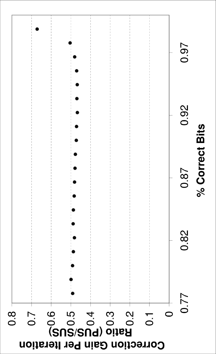
Figure 1: The relative improvement in correct bits for PUS/SUS as a function of the current percentage of correct bits. Using BSC, $N=3333$ (9999 bits), $R=1/3$, $f=0.23$, $GF(8)$, 10000 samples and a 2-S Markov source.

References

- [1] R. G. Gallager, “Low density parity check codes,” IRE Trans. Inform. Theory, vol. 8, pp. 21–28, 1962.
- [2] D. J. C. Mackay and R. M. Neal, “Near shannon limit performance of low density parity check codes,” Elect. Lett., vol. 33, no. 6, pp. 457–458, Mar. 1997.
- [3] J. Pearl, Probabilistic Reasoning in Intelligent Systems: Networks of Plausible Inference. San Francisco: Morgan Kaufmann, 1988.
- [4] M. C. Davey and D. J. C. Mackay, “Low-density parity check codes over GF(q),” IEEE Commun. Lett., vol. 2, no. 6, pp. 165–167, June 1998.
- [5] T. Richardson, A. Shokrollahi, and R. Urbanke, “Design of provably good low-density parity check codes,” IEEE Trans. Inform. Theory, vol. 47, pp. 619–637, Feb. 2001.
- [6] I. Kanter and D. Saad, “Error-correcting codes that nearly saturate shannon’s bound,” Phys. Rev. Lett., vol. 83, no. 13, pp. 2660–2663, Sept. 1999.
- [7] H. Kfir and I. Kanter, “Parallel versus sequential updating for belief propagation decoding,” Physica A, vol. 330, pp. 259–270, Sept. 2003. [Online]. Available: http://xxx.lanl.gov/PS_cache/cond-mat/pdf/0207/0207185.pdf
- [8] J. Zhang, Y. Wang, M. Fossorier, and J. S. Yedidia, “Iterative decoding using replicas,” Mitsubishi Electric Laboratories, Cambridge, MA, Tech. Rep. TR-2005-090, Aug. 2005. [Online]. Available: http://www.merl.com
- [9] S. Tong and X. Wang, “Convergence analysis of Gallager codes under different message-passing schedules,” IEEE Commun. Lett., vol. 9, pp. 249–251, Mar. 2005.
- [10] E. Sharon, S. Litsyn, and J. Goldberger, “Efficient message-assing schedule for LDPC decoding,” in Proc. 23rd IEEE Convention, Tel-Aviv, Israel, Sept. 2004, pp. 223–226.
- [11] J. Zhang and M. Fossorier, “Shuffled belief propagation decoding,” in Proc. 36th Annual Asilomar Conf. on Signals, Systems and Computers, CA, USA, Nov. 2002, pp. 8–15.
- [12] H. Kfir, E. Shpilman, and I. Kanter, “An efficient MN-algorithm for joint source-channel coding,” in Proc. International Symposium on Information Theory and its Applications, ISITA, Parma, Italy, Oct. 2004, pp. 10–13.