Systematic Topology Analysis and Generation
Using Degree Correlations

Abstract

Researchers have proposed a variety of metrics to measure important graph properties, for instance, in social, biological, and computer networks. Values for a particular graph metric may capture a graph’s resilience to failure or its routing efficiency. Knowledge of appropriate metric values may influence the engineering of future topologies, repair strategies in the face of failure, and understanding of fundamental properties of existing networks. Unfortunately, there are typically no algorithms to generate graphs matching one or more proposed metrics and there is little understanding of the relationships among individual metrics or their applicability to different settings.

We present a new, systematic approach for analyzing network topologies. We first introduce the $dK$-series of probability distributions specifying all degree correlations within $d$-sized subgraphs of a given graph $G$. Increasing values of $d$ capture progressively more properties of $G$ at the cost of more complex representation of the probability distribution. Using this series, we can quantitatively measure the distance between two graphs and construct random graphs that accurately reproduce virtually all metrics proposed in the literature. The nature of the $dK$-series implies that it will also capture any future metrics that may be proposed. Using our approach, we construct graphs for $d=0,1,2,3$ and demonstrate that these graphs reproduce, with increasing accuracy, important properties of measured and modeled Internet topologies. We find that the $d=2$ case is sufficient for most practical purposes, while $d=3$ essentially reconstructs the Internet AS- and router-level topologies exactly. We hope that a systematic method to analyze and synthesize topologies offers a significant improvement to the set of tools available to network topology and protocol researchers.

1 Introduction

Knowledge of network topology is crucial for understanding and predicting the performance, robustness, and scalability of network protocols and applications. Routing and searching in networks, robustness to random network failures and targeted attacks, the speed of worms spreading, and common strategies for traffic engineering and network management all depend on the topological characteristics of a given network.

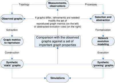
Figure 1: Methodologies of network topology research.

Research involving network topology, particularly Internet topology, generally investigates the following questions:

1. generation: can we efficiently generate ensembles of random but “realistic” topologies by reproducing a set of simple graph metrics?

2. simulations: how does some (new) protocol or application perform on a set of these “realistic” topologies?

3. evolution: what are the forces driving the evolution (growth) of a given network?

Figure 1 illustrates the methodologies used to answer these questions in its left, bottom, and right parts, respectively. Common to all of the methodologies is a set of practically-important graph properties used for analyzing and comparing sets of graphs at the center box of the figure. Many such properties have been defined and explored in the literature. We briefly discuss some of them in Section 2. Unfortunately, there are no known algorithms to construct random graphs with given values of most of these properties, since they typically characterize the global structure of the topology, making it difficult or impossible to algorithmically reproduce them.

This paper introduces a finite set of reproducible graph properties, the $dK$-series, to describe and constrain random graphs in successively finer detail. In the limit, these properties describe any given graph completely. In our approach, we make use of probability distributions, the $dK$-distributions, specifying node degree correlations within subgraphs of size $d$ in some given input graph. We call $dK$-graphs the sets of graphs constrained by given values of $dK$-distributions. Producing a family of $0K$-graphs for a given input graph requires reproducing only the average node degree of the original graph, while producing a family of $1K$-graphs requires reproducing the original graph’s node degree distribution, the $1K$-distribution. $2K$-graphs reproduce the joint degree distribution, the $2K$-distribution, of the original graph—the probability that a randomly selected link connects nodes of degrees $k$ and $k^{\prime}$. $3K$-graphs consider interconnectivity among triples of nodes, and so forth. Generally, the set of $(d+1)K$-graphs is a subset of $dK$-graphs. In other words, larger values of $d$ further constrain the number of possible graphs. Overall, larger values of $d$ capture increasingly complex properties of the original graph. However, generating $dK$-graphs for large values of $d$ also become increasingly computationally complex.

A key contribution of this paper is to define the series of $dK$-graphs and $dK$-distributions and to employ them for generating and analyzing network topologies. Specifically, we develop and implement new algorithms for constructing $2K$- and $3K$-graphs—algorithms to generate $0K$- and $1K$-graphs are already known. For a variety of measured and modeled Internet AS- and router-level topologies, we find that reproducing their $3K$-distributions is sufficient to accurately reproduce all graph properties we have encountered so far.

Our initial experiments suggest that the $dK$-series has the potential to deliver two primary benefits. First, it can serve as a basis for classification and unification of a variety of graph metrics proposed in the literature. Second, it establishes a path towards construction of random graphs matching any complex graph properties, beyond the simple per-node properties considered by existing approaches to network topology generation.

2 Important Topology Metrics

In this section we outline a list of graph metrics that have been found important in the networking literature. This list is not complete, but we believe it is sufficiently diverse and comprehensive to be used as a good indicator of graph similarity in subsequent sections. In addition, our primary concern is how accurately we can reproduce important metrics. One can find statistical analysis of these metrics for Internet topologies in [30] and, more recently, in [20].

The spectrum of a graph is the set of eigenvalues of its Laplacian $\mathcal{L}$. The matrix elements of $\mathcal{L}$ are $\mathcal{L}_{ij}=-1/(k_{i}k_{j})^{1/2}$ if there is a link between a $k_{i}$-degree node $i$ and a $k_{j}$-degree node $j$; otherwise they are $0$, or $1$ if $i=j$. All the eigenvalues lie between 0 and 2. Of particular importance are the smallest non-zero and largest eigenvalues, $\lambda_{1}$ and $\lambda_{n-1}$, where $n$ is the graph size. These eigenvalues provide tight bounds for a number of critical network characteristics [8] including network resilience [29] and network performance [19], i.e., the maximum traffic throughput of the network.

The distance distribution $d(x)$ is the number of pairs of nodes at a distance $x$, divided by the total number of pairs $n^{2}$ (self-pairs included). This metric is a normalized version of expansion [29]. It is also important for evaluating the performance of routing algorithms [18] as well as of the speed with which worms spread in a network.

Betweenness is the most commonly used measure of centrality, i.e., topological importance, both for nodes and links. It is a weighted sum of the number of shortest paths passing through a given node or link. As such, it estimates the potential traffic load on a node or link, assuming uniformly distributed traffic following shortest paths. Metrics such as link value [29] or router utilization [19] are directly related to betweenness.

Perhaps the most widely known graph property is the node degree distribution $P(k)$, which specifies the probability of nodes having degree $k$ in a graph. The unexpected finding in [13] that degree distributions in Internet topologies closely follow power laws stimulated further interest in topology research.

The likelihood $S$ [19] is the sum of products of degrees of adjacent nodes. It is linearly related to the assortativity coefficient $r$ [25] suggested as a summary statistic of node interconnectivity: assortative (disassortative) networks are those where nodes with similar (dissimilar) degrees tend to be tightly interconnected. They are more (less) robust to both random and targeted removals of nodes and links. Li et al. use $S$ in [19] as a measure of graph randomness to show that router-level topologies are not “very random”: instead, they are the result of sophisticated engineering design.

Clustering $C(k)$ is a measure of how close neighbors of the average $k$-degree node are to forming a clique: $C(k)$ is the ratio of the average number of links between the neighbors of $k$-degree nodes to the maximum number of such links ${k\choose 2}$. If two neighbors of a node are connected, then these three nodes form a triangle (3-cycle). Therefore, by definition, $C(k)$ is the average number of 3-cycles involving $k$-degree nodes. Bu and Towsley [4] employ clustering to estimate accuracy of topology generators. More recently, Fraigniaud [14] finds that a wide class of searching/routing strategies are more efficient on strongly clustered networks.

3 dK-series and dK-graphs

There are several problems with the graph metrics in the previous section. First, they derive from a wide range of studies, and no one has established a systematic way to determine which metrics should be used in a given scenario. Second, there are no known algorithms capable of constructing graphs with desired values for most of the described metrics, save degree distribution and more recently, clustering [27]. Metrics such as spectrum, distance distribution, and betweenness characterize global graph structure, while known approaches to generating graphs deal only with local, per-node statistics, such as the degree distribution. Third, this list of metrics is incomplete. In particular, it cannot include any future metrics that may be of interest. Identifying such a metric might result in finding that known synthetic graphs do not match this new metric’s value: moving along the loops in Figure 1 can thus continue forever.

To address these problems, we focus on establishing a finite set of mutually related properties that can form a basis for any topological graph study. More precisely, for any graph $G$, we wish to identify a series of graph properties $\mathcal{P}_{d}$, $d=0,1,\ldots$, satisfying the following requirements:

1. constructibility: we can construct graphs having these properties;

2. inclusion: any property $\mathcal{P}_{d}$ subsumes all properties $\mathcal{P}_{i}$ with $i=0,\ldots,d-1$: that is, a graph having property $\mathcal{P}_{d}$ is guaranteed to also have all properties $\mathcal{P}_{i}$ for $i<d$;

3. convergence: as $d$ increases, the set of graphs having property $\mathcal{P}_{d}$ “converges” to $G$: that is, there exists a value of index $d=D$ such that all graphs having property $\mathcal{P}_{D}$ are isomorphic to $G$.

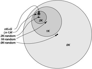
Figure 2: The $dK$- and $dK$-random graph hierarchy. The circles represent $dK$-graphs, whereas their centers represent $dK$-random graphs. The cross is the $nK$-graph isomorphic to a given graph $G$.

In the rest of this section, we establish our construction of the properties $\mathcal{P}_{d}$, which we will call the $dK$-series. We begin with the observation that the most basic properties of a network topology characterize its connectivity. The coarsest connectivity property is the average node degree $\bar{k}=2m/n$, where $n=|V|$ and $m=|E|$ are the numbers of nodes and links in a given graph $G(V,E)$. Therefore, the first property $\mathcal{P}_{0}$ in our $dK$-series $\mathcal{P}_{d}$ is that the graph’s average degree $\bar{k}$ has the same value as in the given graph $G$. In Figure 2 we schematically depict the set of all graphs having property $\mathcal{P}_{0}$ as $0K$-graphs, defining the largest circle. Generalizing, we adopt the term $dK$-graphs to represent the set of all graphs having property $\mathcal{P}_{d}$.

The $\mathcal{P}_{0}$ property tells us the average number of links per node, but it does not tell us the distribution of degrees across nodes. In particular, we do not know the number of nodes $n(k)$ of each degree $k$ in the graph. We define property $\mathcal{P}_{1}$ to capture this information: $\mathcal{P}_{1}$ is therefore the property that the graph’s node degree distribution $P(k)=n(k)/n$ has the same form as in the given graph $G$. It is convenient to call $P(k)$ the $1K$-distribution. $\mathcal{P}_{1}$ implies at least as much information about the network as $\mathcal{P}_{0}$, but not vice versa: given $P(k)$, we find $\bar{k}=\sum kP(k)$. $\mathcal{P}_{1}$ provides more information than $\mathcal{P}_{0}$, and it is therefore a more restrictive metric: the set of $1K$-graphs is a subset of the set of $0K$-graphs. Figure 2 illustrates this inclusive relationship by drawing the set of $1K$-graphs inside the set of $0K$-graphs.

Continuing to $d=2$, we note that the degree distribution constrains the number of nodes of each degree in the network, but it does not describe the interconnectivity of nodes with given degrees. That is, it does not provide any information on the total number $m(k,k^{\prime})$ of links between nodes of degree $k$ and $k^{\prime}$. We define the third property $\mathcal{P}_{2}$ in our series as the property that the graph’s joint degree distribution (JDD) has the same form as in the given graph $G$. The JDD, or the $2K$-distribution, is $P(k_{1},k_{2})=m(k_{1},k_{2})\mu(k_{1},k_{2})/(2m)$, where $\mu(k_{1},k_{2})$ is 2 if $k_{1}=k_{2}$ and 1 otherwise. The JDD describes degree correlations for pairs of connected nodes. Given $P(k_{1},k_{2})$, we can calculate $P(k)=(\bar{k}/k)\sum_{k^{\prime}}P(k,k^{\prime})$, but not vice versa. Consequently, the set of $2K$-graphs is a subset of the $1K$-graphs. Therefore, Figure 2 depicts the smaller $2K$-graph circle inside $1K$.

We can continue to increase the amount of connectivity information by considering degree correlations among greater numbers of connected nodes. To move beyond $2K$, we must begin to distinguish the various geometries that are possible in interconnecting $d$ nodes. To introduce $\mathcal{P}_{3}$, we require the following two components: 1) wedges: chains of 3 nodes connected by 2 edges, called the $P_{\wedge}(k_{1},k_{2},k_{3})$ component; and 2) triangles: cliques of 3 nodes, called the $P_{\triangle}(k_{1},k_{2},k_{3})$ component:

As the two geometries occur with different frequencies among nodes having different degrees, we require a separate probability distribution for each configuration. We call these two components taken together the $3K$-distribution.

For $\mathcal{P}_{4}$, we need the above six distributions: where instead of indices $\wedge,\triangle$ we use for $d=3$, we have all non-isomorphic graphs of size $4$ numbered by $1,\ldots,6$. We note that the order of $k$-arguments generally matters, although we can permute any pair of arguments corresponding to pairs of nodes whose swapping leaves the graph isomorphic. For example: $P_{\wedge}(k_{1},k_{2},k_{3})\neq P_{\wedge}(k_{2},k_{1},k_{3})\neq P_{\wedge}(k_{1},k_{3},k_{2})$, but $P_{\wedge}(k_{1},k_{2},k_{3})=P_{\wedge}(k_{3},k_{2},k_{1})$.

In the following figure, we illustrate properties $\mathcal{P}_{d}$, $d=0,\ldots,4$, calculated for a given graph $G$ of size $4$, where for simplicity, values of all distributions $P$ are the total numbers of corresponding subgraphs, i.e., $P(2,3)=2$ means that $G$ contains $2$ edges between $2$- and $3$-degree nodes.

Generalizing, we define the $dK$-distributions to be degree correlations within non-isomorphic simple connected subgraphs of size $d$ and the $dK$-series $\mathcal{P}_{d}$ to be the series of properties constraining the graph’s $dK$-distribution to the same form as in a given graph $G$. In other words, $\mathcal{P}_{d}$ tells us how groups of $d$-nodes with degrees $k_{1},...,k_{d}$ interconnect. In the ‘$dK$’ acronym, ‘$K$’ represents the standard notation for node degrees, while ‘$d$’ refers to the number of degree arguments $k$ of the $dK$-distributions $P(k_{1},\ldots,k_{d})$ and to the upper bound of the distance between nodes with specified degree correlations. Moving from $\mathcal{P}_{d}$ to $\mathcal{P}_{d+1}$ in describing a given graph $G$ is somewhat similar to including the additional $d+1$’th term of the Fourier (time) or Taylor series representing a given function $F$. In both cases, we describe wider “neighborhoods” in $G$ or $F$ to achieve a more accurate representation of the original structure.

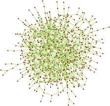
(a) $0K$-graph

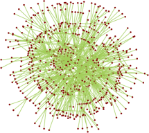
(b) $1K$-graph

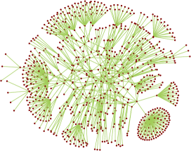
(c) $2K$-graph

(d) $3K$-graph

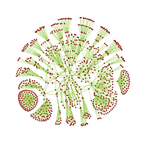
(e) original HOT graph

Figure 3: Picturizations of $dK$-graphs and the original HOT graph illustrating the convergence of $dK$-series.

The $dK$-series definition satisfies the inclusion and convergence requirements described above. Indeed, the inclusion requirement is satisfied because any graph of size $d$ is a subgraph of some graph of size $d+1$. Convergence follows from the observation that in the limit of $d=n$, the set of $nK$-graphs contains only one element: $G$ itself. As a consequence of the convergence property, any topology metric we can define on $G$ will eventually be captured by $dK$-graphs with a sufficiently large $d$.

Hereafter, our main concerns with the $dK$-series become: 1) how well we can satisfy our first requirement of constructibility and 2) how fast the $dK$-series converges toward the original graph. We address these two concerns in Sections 4 and 5.

The reason for the second concern is that the number of probability distributions required to fully specify the $dK$-distribution grows quickly with $d$: see [28] for the number of non-isomorphic simple connected graphs of size $d$. Relative to the existing work on topology generators typically limited to $d=1$ [1, 22, 32], we introduce and implement algorithms for graph construction for  $d=2$ and $d=3$. We present these algorithms in Section 4 and then show in Section 5 that the $dK$-series converges quickly: $2K$-graphs are sufficient for most practical purposes for the graphs we consider, while $3K$-graphs are essentially identical to observed and modeled Internet topologies.

To motivate our ability to capture increasingly complex graph properties by increasing $d$, we present visualizations of $dK$-graphs generated using the $dK$-randomizing approach we will discuss in Section 4.1.4. Figure 3 depicts random $0K$-, $1K$-, $2K$- and $3K$-graphs matching the corresponding distributions of the HOT graph, a representative router-level topology from [19]. This topology is particularly interesting, because, to date reproducing router-level topologies using only degree distributions has proven difficult [19]. However, a visual inspection of our generated topologies shows good convergence properties of the $dK$-series: while the $0K$-graph and $1K$-graph have little resemblance with the HOT topology, the $2K$-graph is much closer than the previous ones and the $3K$ graph is almost identical to the original. Although the visual inspection is encouraging, we defer more careful comparisons to Section 5.

4 Constructing dK-graphs

There are several approaches for constructing $dK$-graphs for $d=0$ and $d=1$. We extended a number of these algorithms to work for higher values of $d$. In Section 4.1, we describe these approaches, their practical utility, and our new algorithms for $d>1$. In Sections 4.2 and 4.3, we introduce $dK$-random graphs and $dK$-space explorations. We use the latter to determine the lowest values of $d$ such that $dK$-graphs approximate a given topology with the required degree of accuracy.

4.1 $dK$-graph-constructing algorithms

We classify existing approaches to constructing $0K$- and $1K$-graphs into the following categories: stochastic, pseudograph, matching, and two types of rewiring: randomizing and targeting. We attempted to extend each of these techniques to general $dK$-graph construction. In this section, we qualitatively discuss the relative merits of each of these approaches before presenting a more quantitative comparison in Section 5.

4.1.1 Stochastic

The simplest and most convenient for theoretical analysis is the stochastic approach. For $0K$, reproducing an $n$-sized graph with a given expected average degree $\bar{k}$ involves connecting every pair of $n$ nodes with probability $p_{0K}=\bar{k}/n$. This construction forms the classical (Erdős-Rényi) random graphs $\mathcal{G}_{n,p}$ [12]. Recent efforts have extended this stochastic approach to $1K$ [7] and $2K$ [2, 9]. In these cases, one first labels all nodes $i$ with their expected degrees $q_{i}$ drawn from the distribution $P(k)$ and then connects pairs of nodes $(i,j)$ with probabilities $p_{1K}(q_{i},q_{j})=q_{i}q_{j}/(n\bar{q})$ or $p_{2K}(q_{i},q_{j})=(\bar{q}/n)P(q_{i},q_{j})/(P(q_{i})P(q_{j}))$ reproducing the expected values of $1K$- or $2K$-distributions, respectively.

In theory, we could generalize this approach for any $d$ in two stages: 1) extraction: given a graph $G$, calculate the frequencies of all (including disconnected) $d$-sized subgraphs in $G$, and 2) construction: prepare an $n$-sized set of $q_{i}$-labeled nodes and connect their $d$-sized subsets into different subgraphs with (conditional) probabilities based on the calculated frequencies. In practice, we find the stochastic approach performs poorly even for $1K$ because of high statistical variance. For example, many nodes with expected degree $1$ wind up with degree $0$ after the construction phase, resulting in many tiny connected components.

4.1.2 Pseudograph

The pseudograph (also known as configuration) approach is probably the most popular and widely used class of graph-generating algorithms. In its original form [1, 24], it applies only to the $1K$ case. Relative to the stochastic approach, it reproduces a given degree distribution exactly, but does not necessarily construct simple graphs. That is, it may construct graphs with both ends of an edge connected to the same node (self-loops) and with multiple edges between the same pair of nodes (loops).

It operates as follows. Given the number of nodes, $n(k)$, of degree $k$, $n=\sum_{k=1}^{k_{\max}}n(k)$, first prepare $n(k)$ nodes with $k$ stubs attached to each node, $k=1,\ldots,k_{\max}$, and then randomly choose pairs of stubs and connect them to form edges. To obtain a simple connected graph, remove all loops and extract the largest connected component.

We extended this algorithm to $2K$ as follows. Given the number $m(k_{1},k_{2})$ of edges between $k_{1}$- and $k_{2}$-degree nodes, $m=\sum_{k_{1},k_{2}=1}^{k_{\max}}m(k_{1},k_{2})$, we first prepare lists of $m(k_{1},k_{2})$ disconnected edges and label the both ends of each edge by $k_{1}$ and $k_{2}$, $k_{1},k_{2}=1,\ldots,k_{\max}$. Next, for each $k$, $k=1,\ldots,k_{\max}$, we create a list of all edge-ends labeled with $k$. From this list, we randomly select groups of $k$ edge-ends to form the $k$-degree nodes in the final graph.

The pseudograph algorithm works well for $d=2$. Unfortunately, we could not easily generalize it for $d>2$ because starting at $d=3$, $d$-sized subgraphs overlap over edges. Such overlapping introduces a series of topological constraints and non-local dependencies among different subgraphs, and we could not find a simple technique to preserve these combinatorial constraints during the construction phase.

4.1.3 Matching

The matching approach differs from the pseudograph approach in avoiding loops during the construction phase. In the $1K$ case, the algorithm works exactly as its pseudograph counterpart but skips pairs of stubs that form loops if connected. We extend the matching approach to $2K$ in a manner similar to our $2K$ pseudograph approach.

Unfortunately, loop avoidance suffers from various forms of deadlock for both $1K$ and $2K$. In both cases, the algorithms can end up in incomplete configurations when not all edges are formed, and the graph cannot be completed because there are no suitable stub pairs remaining that can be connected without forming loops. We devised several techniques to deal with these problems. With these additional techniques, we obtained good results for $2K$ graphs. As in the pseudograph case however, we could not generalize matching for $d>2$ for essentially the same reasons related to subgraphs’ overlapping and non-locality.

4.1.4 Rewiring

The rewiring approaches are generalizable to any $d$ and work well in practice. They involve $dK$-preserving rewiring as illustrated in Figure 4.

Figure 4: $dK$-preserving rewiring for $d=0,1,2$.

The main idea is to rewire random (pairs of) edges preserving an existing form of the $dK$-distribution. For $d=0$, we rewire a random edge to a random pair of nodes, thus preserving $\bar{k}$. For $d=1$, we rewire two random edges that do not alter $P(k)$, as shown in Figure 4. If, in addition, there are at least two nodes of equal degrees adjacent to the different edges in the edge pair, then the same rewiring leaves $P(k,k^{\prime})$ intact. Due to the inclusion property of the $dK$-series, $(d+1)K$-rewirings form a subset of $dK$-rewirings for $d>0$. For example, to preserve $3K$, we permit a $2K$-rewiring only if it also preserves the wedge and triangle distributions.

The $dK$-randomizing rewiring algorithm amounts to performing $dK$-preserving rewirings a sufficient number of times for some $dK$-graph. A “sufficient number” means enough rewirings for this process to lead to graphs that do not change their properties even if we subject them to additional rewirings. In other words, this rewiring process converges after some number of steps, producing random graphs having property $\mathcal{P}_{d}$. Even for $d=1$, there are no known rigorous results regarding how quickly this process converges, but [15] shows that this process is an irreducible, symmetric and aperiodic Markov chain and demonstrates experimentally that it takes $O(m)$ steps to converge.

In our experiments in Section 5, we employ the following strategy applicable for any $d$. We first calculate the number of possible initial $dK$-preserving rewirings. By “initial rewirings” we mean rewirings we can perform on a given graph $G$, to differentiate them from rewirings we can apply to graphs obtained from $G$ after its first (and subsequent) rewirings. We then subtract the number of rewirings that leave the graph isomorphic. For example, rewiring of any two $(1,k)$- and $(1,k^{\prime})$-edges is a $dK$-preserving rewiring, for any $d$, and more strongly, the graph before rewiring is isomorphic to the graph after rewiring. We multiply this difference by $10$, and perform that number of random rewirings. At the end of our rewiring procedure, we explicitly verify that randomization is indeed complete and the process has converged by further increasing the number of rewirings and checking that all graph characteristics remain unchanged.

One obvious problem with $dK$-randomization is that it requires an original graph $G$ as input to construct its $dK$-random versions. It cannot start with a description of the $dK$-distribution to generate random $dK$-graphs as is possible with the other construction approaches discussed above.

To address this limitation, we consider the inverse process of $dK$-targeting $d^{\prime}K$-preserving rewiring, also known as Metropolis dynamics [23]. It incorporates the following modification to $d^{\prime}K$-preserving rewiring: every rewiring step is accepted only if it moves the graph “closer” to $\mathcal{P}_{d}$. In practice, we can then employ targeting rewiring to construct $dK$-graphs with high values of $d$ by beginning with any $d^{\prime}K$-graph where $d^{\prime}<d$. Recall that we can always compute $\mathcal{P}_{d^{\prime}}$ from $\mathcal{P}_{d}$ due to the inclusion property of the $dK$-series. For instance, we can start with a graph having a given degree distribution ($d^{\prime}=1$) [31], and then move it toward a $dK$-graph via $dK$-targeting $1K$-preserving rewiring.

The definition of “closer” above requires further explanation. We require a set of distance metrics that quantitatively differentiate two graphs based on the values of their $dK$-distributions. In our experiments, we use the sum of squares of differences between the existing and target numbers of subgraphs of a given type. For example, in the $d=2$ case, we measure the distance between the target graph’s JDD and the JDD of the current graph being rewired by $\mathcal{D}_{2}=\sum_{k_{1},k_{2}}\left[m_{\mathrm{current}}(k_{1},k_{2})-m_{\mathrm{target}}(k_{1},k_{2})\right]^{2}$, and at each rewiring step, we accept the rewiring only if it decreases this distance. Note that $\mathcal{D}_{2}$ is non-negative and equals zero only when reaching the target JDD. For $d=3$, this distance $\mathcal{D}_{3}$ is a sum of squares of differences between the current and target numbers of wedges and triangles, and we can generalize it to $\mathcal{D}_{d}$ for any $d$.

A potential problem with $dK$-targeting $d^{\prime}K$-preserving rewiring is that it can be nonergodic, meaning that there might be no chain of $d^{\prime}K$-preserving $\mathcal{D}_{d}$-decreasing rewirings leading from the initial $d^{\prime}K$-graph to the target $dK$-graph. In other words, we cannot be sure beforehand that any two $d^{\prime}K$-graphs are connected by a sequence of $d^{\prime}K$-preserving and $\mathcal{D}_{d}$-decreasing rewirings.

To address this problem we note that the $d^{\prime}K$-randomizing and $dK$-targeting $d^{\prime}K$-preserving rewirings are actually two extremes of an entire family of rewiring processes. Indeed, let $\Delta\mathcal{D}_{d}=\mathcal{D}_{d,\mathrm{after}}-\mathcal{D}_{d,\mathrm{before}}$ be the difference of distance to the target $dK$-distribution computed before and after a $d^{\prime}K$-preserving rewiring step. As with the usual $dK$-targeting rewiring, we accept a rewiring step if $\Delta\mathcal{D}_{d}<0$, but even if $\Delta\mathcal{D}_{d}\geqslant 0$, we also accept this step with probability $e^{-\Delta\mathcal{D}_{d}/T}$, where $T>0$ is some parameter that we call temperature because of the similarity of the process to simulated annealing.

In the $T\to 0$ limit, this probability goes to $0$, and we have the standard $dK$-targeting $d^{\prime}K$-preserving rewiring process. When $T\to\infty$, the probability approaches $1$, yielding the standard $d^{\prime}K$-randomizing rewiring process. To verify ergodicity, we can start with a high temperature and then gradually cool the system while monitoring any metric known to have different values in $dK$- and $d^{\prime}K$-graphs. If this metric’s value forms a continuous function of the temperature, then our rewiring process is ergodic. Maslov et al. performed these experiments in [21] and demonstrated ergodicity in the case with $d^{\prime}=1$ and $d=2$. In our experiments in Section 5 where $d$ and $d^{\prime}$ are below $4$, we always obtain a good match for all target graph metrics. Thus, we perform rewiring at zero temperature without further considering ergodicity. If however in some future experiments one detects the lack of a smooth convergence of rewiring procedures, then one should first verify ergodicity using the methodology described above.

For all the algorithms discussed in this section, we do not check for graph connectedness at each step of the algorithm since: 1) it is an expensive operation and 2) all resulting graphs always have giant connected components (GCCs) with characteristics similar to the whole disconnected graphs.

4.2 $dK$-random graphs

Table 1: The summary of $dK$-series.

Tag $dK$	Property symbol	$dK$-distribution	$\mathcal{P}_{d}$ defines $\mathcal{P}_{d-1}$	Edge existence probability in stochastic constructions	Maximum entropy value of $(d+1)K$-distribution in $dK$-random graphs
$0K$	$\mathcal{P}_{0}$	$\bar{k}$		$p_{0K}=\bar{k}/n$	$P_{0K}(k)=e^{-\bar{k}}\bar{k}^{k}/k!$
$1K$	$\mathcal{P}_{1}$	$P(k)$	$\bar{k}=\sum kP(k)$	$p_{1K}(q_{1},q_{2})=q_{1}q_{2}/(n\bar{q})$	$P_{1K}(k_{1},k_{2})=k_{1}P(k_{1})k_{2}P(k_{2})/\bar{k}^{2}$
$2K$	$\mathcal{P}_{2}$	$P(k_{1},k_{2})$	$P(k)=(\bar{k}/k)\sum_{k^{\prime}}P(k,k^{\prime})$	$p_{2K}(q_{1},q_{2})=(\bar{q}/n)P(q_{1},q_{2})/(P(q_{1})P(q_{2}))$	See [10] for clustering in $2K$-random graphs
$3K$	$\mathcal{P}_{3}$	$P_{\wedge}(k_{1},k_{2},k_{3})$ $P_{\triangle}(k_{1},k_{2},k_{3})$	By counting edges, we get $P(k_{1},k_{2})\sim\sum_{k}\left\{P_{\wedge}(k,k_{1},k_{2})+P_{\triangle}(k,k_{1},k_{2})\right\}/(k_{1}-1)\sim\sum_{k}\left\{P_{\wedge}(k_{1},k_{2},k)+P_{\triangle}(k_{1},k_{2},k)\right\}/(k_{2}-1)$, where we omit normalization coefficients.
…	…	…	…	…	…
$nK$	$\mathcal{P}_{n}$	$G$

No $dK$-graph-generating algorithm can quickly construct the set of all $dK$-graphs because: 1) such sets are too large, especially for small $d$; and, less obviously, 2) all algorithms try to produce graphs having property $\mathcal{P}_{d}$ while remaining unbiased (random) with respect to all other properties. One can check directly that the last characteristic applies to all the algorithms we have discussed above.

As a consequence, the $dK$-graph construction algorithms result in non-uniform sampling of graphs with different values of properties that are not fully defined by $\mathcal{P}_{d}$. More specifically, two generated $dK$-graphs having different forms of a $d^{\prime}K$-distribution with $d^{\prime}>d$ can appear as the output of these algorithms with drastically different probabilities. Some $dK$-graphs have such a small probability of being constructed that we can safely assume they never arise.

For example, consider the simplest $0K$ stochastic construction, i.e., the classical random graphs $\mathcal{G}_{n,p}$. Using a probabilistic argument, one can show that the naturally-occurring $1K$-distribution (degree distribution) in these graphs has a specific form: binomial, which is closely approximated by the Poisson distribution: $P_{0K}(k)=e^{-\bar{k}}\bar{k}^{k}/k!$ [11]. The $0K$ stochastic algorithm may produce a graph with a different $1K$-distribution, e.g., the power-law $P(k)\sim k^{-\gamma}$, but the probability of such an outcome is extremely low. Indeed, suppose $n\sim 10^{4}$, $\bar{k}\sim 5$, and $\gamma\sim 2.1$, so that the characteristic maximum degree is $k_{\max}\sim 2000$ (we chose these values to reflect measured values for Internet AS topologies). In this case, the probability that a $\mathcal{G}_{n,p}$-graph contains at least one node with degree equal to $k_{\max}$ is dominated by $1/2000!\sim 10^{-6600}$, and the probability that the remaining degrees simultaneously match those required for a power law is much lower.

It is thus natural to introduce a set of graphs that correspond to the graphs most likely to be generated by $dK$-graph constructing algorithms. We call such graphs the $dK$-random graphs. These graphs have property $\mathcal{P}_{d}$ but are unbiased with respect to any other more constraining property. In this sense, the $dK$-random graphs are the maximally random or maximum-entropy $dK$-graphs. Our term maximum entropy here has the following justification. As we have just seen, $0K$-random graphs have the maximum-entropy value of the $1K$-distribution since their node degree distribution is the distribution with the maximum entropy among all the distributions with a fixed average. The $1K$-random graphs have the maximum-entropy value of the $2K$-distribution since their joint degree distribution, $P_{1K}(k_{1},k_{2})=\tilde{P}(k_{1})\tilde{P}(k_{2})$, where $\tilde{P}(k)=kP(k)/\bar{k}$ [11], is the distribution with the maximum joint entropy (minimum mutual information) among all the joint distributions with fixed marginal distributions.

The main point we extract from these observations is that in trying to construct $dK$-graphs, we generally obtain graphs from subsets of the $dK$-space. We call these subsets $dK$-random graphs and schematically depict them as centers of the $dK$-circles in Figure 2. These graphs do have property $\mathcal{P}_{d}$ and, consequently, properties $\mathcal{P}_{i}$ with $i<d$, but they might not ever display property $\mathcal{P}_{j}$ with $j>d$ since their $jK$-distributions have specific, maximum-entropy values that may be different from the $jK$-distribution values in the original graph.

4.3 $dK$-space explorations

Often we wish to analyze the topological constraints a given graph $G$ appears to obey. In other cases, we are interested in exploring the structural diversity among $dK$-graphs. If we are attempting to determine the minimum $d$ such that all $dK$-graphs are similar to $G$, we can start with a small value of $d$, generate $dK$-graphs, and measure their “distance” from $G$. If the distance is too great, we can increase $d$ and repeat the process. On the other hand, to explore structural diversity among all $dK$-graphs, we must generate $dK$-graphs that are not random. These non-random $dK$-graphs are still constrained by $\mathcal{P}_{d}$ but have extremely low probabilities of being generated by unperturbed $dK$-graph constructing algorithms.

We cannot construct all $dK$-graphs, so we need to use heuristics to generate some $dK$-graphs and adjust them according to a distance metric that draws us closer to the types of $dK$-graphs we seek. One such heuristic is based on the inclusion feature of the $dK$-series. Because all $dK$-graphs have the same values of $dK$- but not of $(d+1)K$-distributions, we look for simple metrics fully defined by $\mathcal{P}_{d+1}$ but not by $\mathcal{P}_{d}$. While identifying such metrics can be challenging for high $d$’s, we can always retreat to the following two simple extreme metrics:

• the correlation of degrees of nodes located at distance $d$;

• the concentration of $d$-simplices (cliques of size $d+1$).

These metrics are “extreme” in the sense that they correspond to the $(d+1)$-sized subgraphs with, respectively, the maximum ($d$) and minimum ($1$) possible diameter. We can then construct $dK$-graphs with extreme values, e.g., the smallest or largest possible, for these (extreme) metrics. The $dK$-random graphs have the values of these metrics lying somewhere in between the extremes.

If the goal is to find the smallest $d$ that results in sufficiently constraining graphs, we can compute the difference between the extreme values of these metrics, as well as of other metrics we might consider. If this difference is too large, then the selected value of $d$ is not constraining enough and we need to increase it. If the goal is to visit exotic locations in a large space of $dK$-graphs, then such $dK$-space exploration may be used to move beyond the relatively small circle of $dK$-random graphs.

To illustrate this approach in practice, we consider $1K$- and $2K$-space explorations. For $1K$, the simplest metric defined by $\mathcal{P}_{2}$ is any scalar summary statistics of the $2K$-distribution, such as likelihood $S$ (cf. Section 2). To construct graphs with the maximum value of $S$, we can run a form of targeting $1K$-preserving rewiring that accepts each rewiring step only if it increases $S$. We can perform the opposite to minimize $S$. This type of experiment was at the core of recent work that led the authors of [19] to conclude that $d=1$ was not constraining enough for the topology they considered.

To perform $2K$-space explorations, we need to find simple scalar metrics defined by $\mathcal{P}_{3}$. Since the $3K$-distribution is actually two distributions, $P_{\wedge}(k_{1},k_{2},k_{3})$ and $P_{\triangle}(k_{1},k_{2},k_{3})$, we should have two independent scalar metrics. The second-order likelihood $S_{2}$ is one such metric for $P_{\wedge}(k_{1},k_{2},k_{3})$. We define it as the sum of the products of degrees of nodes located at the ends of wedges, $S_{2}\sim\sum_{k_{1},k_{2},k_{3}}k_{1}k_{3}P_{\wedge}(k_{1},k_{2},k_{3})$. Any graphs with the same $P_{\wedge}(k_{1},k_{2},k_{3})$ have the same $S_{2}$. For the $P_{\triangle}(k_{1},k_{2},k_{3})$ component, average clustering $\bar{C}\sim\sum_{k_{1},k_{2},k_{3}}k_{1}P_{\triangle}(k_{1},k_{2},k_{3})$ is an appropriate candidate. We note that these two metrics are also the two extreme metrics in the sense defined above: $S_{2}$ measures the properly normalized correlation of degrees of nodes located at distance $2$, while $\bar{C}$ describes the concentration of $2$-simplices (triangles). The $2K$-explorations amount then to performing the following two types of targeting $2K$-preserving rewiring: accept a $2K$-rewiring step only if it maximizes or minimizes: 1) $S_{2}$, or 2) $\bar{C}$.

5 Evaluation

In this section, we conduct a number of experiments to demonstrate the ability of the $dK$-series to capture important graph properties. We implemented all the $dK$-graph-constructing algorithms from Section 4.1, applied them to both measured and modeled Internet topologies, and calculated all the topology metrics from Section 2 on the resulting graphs.

We experimented with three measured AS-level topologies, extracted from CAIDA’s skitter traceroute [5], RouteViews’ BGP [26], and RIPE’s WHOIS [17] data for the month of March 2004, as well as with a synthetic router-level topology—the HOT graph from [19]. The qualitative results of our experiments are similar for the skitter and BGP topologies, while the WHOIS topology lies somewhere in-between the skitter/BGP and HOT topologies. In the case of skitter comprising of 9204 nodes and 28959 edges, we will see that its degree distribution places significant constraints upon the graph generation process. Thus, even $1K$-random graphs approximate the skitter topology reasonably well. The HOT topology with 939 nodes and 988 edges is at the opposite extreme. It is the least constrained; $1K$-random graphs approximate it poorly, and $dK$-series’ convergence is slowest. We thus report results only for these two extreme cases, skitter and HOT.

Our results represent averages over 100 graphs generated with a different random seed in each case, using the notation in Table 2.

Table 2: Scalar graph metrics notations.

Metric	Notation
Average degree	$\bar{k}$
Assortativity coefficient	$r$
Average clustering	$\bar{C}$
Average distance	$\bar{d}$
Standard deviation of distance distribution	$\sigma_{d}$
Second-order likelihood	$S_{2}$
Smallest eigenvalue of the Laplacian	$\lambda_{1}$
Largest eigenvalue of the Laplacian	$\lambda_{n-1}$

5.1 Algorithmic Comparison

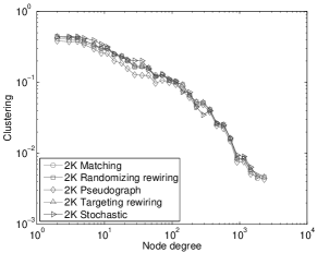
(a) Clustering in skitter for different $2K$ algorithms

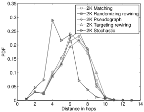
(b) Distance distribution in HOT for different $2K$ algorithms

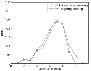
(c) Distance distribution in HOT for different $3K$ algorithms

Figure 5: Comparison of $2K$- and $3K$-graph-constructing algorithms.

Table 3: Scalar metrics for $2K$-random HOT graphs generated using different techniques.

Met-	Stoch-	Pseu-	Match-	$2K$-	$2K$-	Orig.
ric	astic	dogr.	ing	rand.	targ.	HOT
$\bar{k}$	2.87	2.19	2.22	2.18	2.18	2.10
$r$	-0.22	-0.24	-0.21	-0.23	-0.24	-0.22
$\bar{d}$	4.99	6.25	6.22	6.32	6.35	6.81
$\sigma_{d}$	0.85	0.75	0.74	0.70	0.70	0.57

Table 4: Scalar metrics for $3K$-random HOT graphs generated using different techniques.

Metric	$3K$-randomizing	$3K$-targeting	Original
	rewiring	rewiring	HOT
$\bar{k}$	2.10	2.13	2.10
$r$	-0.22	-0.23	-0.22
$\bar{d}$	6.55	6.79	6.81
$\sigma_{d}$	0.84	0.72	0.57

We first compare the different graph generation algorithms discussed in Section 4.1. All the algorithms give consistent results, except the stochastic approach, which suffers from the problems related to high statistical variance discussed in Section 4.1.1. This conclusion immediately follows from Figure 5 and Tables 3 and 4 showing graph metric values for the different $2K$ and $3K$ algorithms described in Section 4.1.

In our experience, we find that $dK$-randomizing rewiring is easiest to use. However, it requires the original graph as input. If only the target $dK$-distribution is available and if $d\leqslant 2$, we find the pseudograph algorithm most appropriate in practice. We note that our $2K$ version results in fewer pseudograph “badnesses”, i.e., (self-)loops and small connected components (CCs), than PLRG [1], its commonly-known $1K$ counterpart. This improvement is due to the additional constraints introduced by the $2K$ case. For example, if there is only one node of high degree $x$ and one node of another high degree $y$ in the original graph, then there can be only one link of type $(x,y)$. Our $2K$ modification of the pseudograph algorithm must consequently produce exactly one link between these two $x$- and $y$-degree nodes, whereas in the $1K$ case, the algorithm tends to create many such links. Similarly, a $1K$ generator tends to produce many pairs of isolated $1$-degree nodes connected to each another. Since the original graph does not have such pairs, i.e., (1,1)-links, our $2K$ generator, as opposed to $1K$, does not form these small $2$-node CCs either.

While the pseudograph algorithm is a good $2K$-random graph generator, we could not generalize it for $d\geqslant 3$ (see Section 4.1.2). Therefore, to generate $dK$-random graphs with $d\geqslant 3$ when an original graph is unavailable, we use $dK$-targeting rewiring. We first bootstrap the process by constructing $1K$-random graphs using the pseudograph algorithm and then apply $2K$-targeting $1K$-preserving rewiring to obtain $2K$-random graphs. To produce $3K$-random graphs, we apply $3K$-targeting $2K$-preserving rewiring to the $2K$-random graphs obtained at the previous step.

5.2 Topology Comparisons

We next test the convergence of our $dK$-series for the skitter and HOT graphs. Since all $dK$-graph constructing algorithms yield consistent results, we selected the simplest one, the $dK$-randomizing rewiring from Section 4.1.4, to obtain $dK$-random graphs in this section.

The number of possible initial $dK$-randomizing rewirings is a good preliminary indicator of the size of the $dK$-graph space. We show these numbers for the HOT graph in Table 5. If we discard rewirings leading to obvious isomorphic graphs, cf. Section 4.1.4, then the number of possible initial rewirings is even smaller.

Table 5: Numbers of possible initial $dK$-randomizing rewirings for the HOT graph.

$d$	Possible initial	Possible initial rewirings,
	rewirings	ignoring obvious isomorphisms
0	435,546,699	-
1	477,905	440,355
2	326,409	268,871
3	146	44

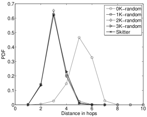
(a) Distance distribution

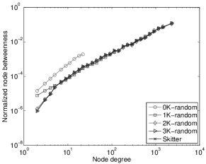
(b) Betweenness

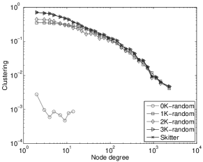
(c) Clustering

Figure 6: Comparison of $dK$-random and skitter graphs.

Table 6: Comparing scalar metrics for $dK$-random and skitter graphs.

Metric	$0K$	$1K$	$2K$	$3K$	skitter
$\bar{k}$	6.31	6.34	6.29	6.29	6.29
$r$	0	-0.24	-0.24	-0.24	-0.24
$\bar{C}$	0.001	0.25	0.29	0.46	0.46
$\bar{d}$	5.17	3.11	3.08	3.09	3.12
$\sigma_{d}$	0.27	0.4	0.35	0.35	0.37
$\lambda_{1}$	0.2	0.03	0.15	0.1	0.1
$\lambda_{n-1}$	1.8	1.97	1.85	1.9	1.9

We compare the skitter topology with its $dK$-random counterparts, $d=0,\ldots,3$, in Table 6 and Figure 6. We report all the metrics calculated for the giant connected component (GCCs). Minor discrepancies between values of average degree $\bar{k}$ and $r$ result from GCC extractions. If we do not extract the GCC, then $\bar{k}$ is the same as that of the original graph for all $d=0,\ldots,3$, and $r$ is exactly the same for $d>1$.

We do not show degree distributions for brevity. However, degree distributions match when considering the entire graph and are very similar for the GCCs for all $d>0$. When $d=0$, the degree distribution is binomial, as expected.

We see that all other metrics gradually converge to those in the original graph as $d$ increases. A value of $d=1$ provides a reasonably good description of the skitter topology, while $d=2$ matches all properties except clustering. The $3K$-random graphs are identical to the original for all metrics we consider, including clustering.

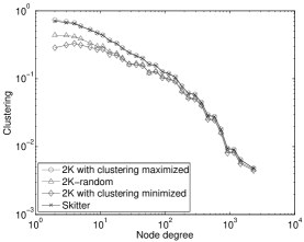
Figure 7: Varying clustering in $2K$-graphs for skitter.

Figure 8: Distance distribution for $dK$-random and HOT graphs

Figure 9: Betweenness for $dK$-random and HOT graphs

We perform the $2K$-space explorations described in Section 4.3 to check if $d=2$ is indeed sufficiently constraining for the skitter topology. We observe small variations of clustering $\bar{C}$, second-order likelihood $S_{2}$, and spectrum, shown in Table 7 and Figure 9. All other metrics do not change, so we do not show plots for them. We conclude that $d=2$, i.e., the joint degree distribution provides a reasonably accurate description of observed AS-level topologies.

Table 7: Scalar metrics for $2K$-space explorations for skitter.

Metric	Min	Max	Min	Max	$2K$-	Skit-
	$\bar{C}$	$\bar{C}$	$S_{2}$	$S_{2}$	rand.	ter
$\bar{k}$	6.29	6.29	6.29	6.29	6.29	6.29
$r$	-0.24	-0.24	-0.24	-0.24	-0.24	-0.24
$\bar{C}$	0.21	0.47	0.4	0.4	0.29	0.46
$\bar{d}$	3.06	3.12	3.12	3.10	3.08	3.12
$\sigma_{d}$	0.33	0.38	0.37	0.36	0.35	0.37
$\lambda_{1}$	0.25	0.11	0.11	0.1	0.15	0.1
$\lambda_{n-1}$	1.75	1.89	1.89	1.89	1.85	1.9
$S_{2}/S_{2}^{\max}$	0.988	0.961	0.955	1.000	0.986	0.958

The HOT topology is more complex than AS-level topologies. Earlier work argues that this topology cannot be accurately modeled using degree distributions alone [19]. We therefore selected the HOT topology graph as a difficult case for our approach.

A preliminary inspection of visualizations in Figure 3 indicates that the $dK$-series converges at a reasonable rate even for the HOT graph. The $0K$-random graph is a classical random graph and lacks high-degree nodes, as expected. The $1K$-random graph has all the high-degree nodes we desire, but they are crowded toward the core, a property absent in the HOT graph. The $2K$ constraints start pushing the high-degree nodes away to the periphery, while the lower-degree nodes migrate to the core, and the $2K$-random graph begins to resemble the HOT graph. The $3K$-random topology looks remarkably similar to the HOT topology.

Of course, visual inspection of a small number of randomly generated graphs is insufficient to demonstrate our ability to capture important metrics of the HOT graph. Thus, we compute the different metric values for each of the $dK$-random graph and compare them with the corresponding value for the original HOT graph. In Table 8 and Figures 9 and 9 we see that the $dK$-series converges more slowly for HOT than for skitter. Note that we do not show clustering plots because clustering is almost zero everywhere: the HOT topology has very few cycles; it is almost a tree. The $1K$-random graphs yield a poor approximation of the original topology, in agreement with the main argument in [19]. Both Figures 3 and 9 indicate that starting with $d=2$, low- but not high-degree nodes form the core: betweenness is approximately as high for nodes of degree $\sim 10$ as for high-degree nodes. Consequently, the $2K$-random graphs provide a better approximation, but not nearly as good as it was for skitter. However, the $3K$-random graphs match the original HOT topology almost exactly. We thus conclude that the $dK$-series captures the essential characteristics of even particularly difficult topologies, such as HOT, by sufficiently increasing $d$, in this case to 3.

Table 8: Comparing scalar metrics for $dK$-random and HOT graphs.

Metric	$0K$	$1K$	$2K$	$3K$	HOT
$\bar{k}$	2.47	2.59	2.18	2.10	2.10
$r$	-0.05	-0.14	-0.23	-0.22	-0.22
$\bar{C}$	0.002	0.009	0.001	0	0
$\bar{d}$	8.48	4.41	6.32	6.55	6.81
$\sigma_{d}$	1.23	0.72	0.71	0.84	0.57
$\lambda_{1}$	0.01	0.034	0.005	0.004	0.004
$\lambda_{n-1}$	1.989	1.967	1.996	1.997	1.997

6 Discussion and Future Work

While we feel our approach to topology analysis holds significant promise, a number of important avenues remain for further investigation. First, one must determine appropriate values of $d$ to carry out studies of interest. Our experience to date suggests that $d=2$ is sufficient to reproduce most metrics of interest and that $d=3$ faithfully reproduces all metrics we are aware of for Internet-like graphs. It also appears likely that $d=3$ will be sufficient for self-organized small-worlds in general. This issue is particularly important because the computational complexity of producing $dK$-graphs grows rapidly with $d$. Studies requiring large values of $d$ may limit the practicality of our approach.

In general, more complex topologies may necessitate developing algorithms for generating $dK$-random graphs with high $d$’s. We needed higher $d$ to describe the HOT topology as accurately as the skitter topology. The intuition behind this observation is that the HOT router-level topology is “less random” because it results from targeted design and engineering. The skitter AS-level topology, on the other hand, is “more random” since there is no single point of external human control over its shape and evolution. It is a cumulative result of local decisions made by individual ASes.

A second important question concerns the discrete nature of our model. For instance, we are able to reproduce $1K$- and $2K$-distributions but it is not meaningful to consider reproducing $1.4K$-distributions. Consider a graph property $X$ not captured by $1K$ but successfully captured by $2K$. It could turn out that the space of $2K$-random graphs over-constrains the set of graphs reproducing $X$. That is, while $2K$-graphs do successfully reproduce $X$, there may be other graphs that also match $X$ but are not $2K$-graphs.

Fundamental to our approach is that we seek to reproduce important characteristics of a given network topology. We cannot use our methodology to discover laws governing the evolutionary growth of a particular network. Rather, we are restricted to observing changes in degree correlations in graphs over time, and then generating graphs that match such degree correlations. However, the goals of reproducing important characteristics of a given set of graphs and discovering laws governing their evolution are complementary and even symmetric.

They are complementary because the $dK$-series can simplify the task of validating particular evolutionary models. Consider the case where a researcher wishes to validate a model for Internet evolution using historical connectivity information. The process would likely involve starting with an initial graph, e.g., reflecting connectivity from five years ago, and generating a variety of larger graphs, e.g., reflecting modern-day connectivity. Of course, the resulting graphs will not match known modern connectivity exactly. Currently, validation would require showing that the graph matches “well enough” for all known ad hoc graph properties. Using the $dK$-series however, it is sufficient to demonstrate that the resulting graphs are $dK$-random for an appropriate value of $d$, i.e., constrained by the $dK$-distribution of modern Internet graphs, with $d=3$ known to be sufficient in this case. As long as the resulting graphs fall in the $dK$-random space, the nature of $dK$-randomness explains any graph metric variation from ground truth. This methodology also addresses the issue of defining “well enough” above: $dK$-space exploration can quantify the expected variation in ad hoc properties not fully specified by a particular $dK$-distribution.

The two approaches are symmetric in that they both attempt to generate graph models that accurately capture values of topology metrics observed in real networks. Both approaches have inherent tradeoffs between accuracy and complexity. Achieving higher accuracy with the $dK$-series requires greater numbers of statistical constraints with increasing $d$. The number of these constraints is upper-bounded by $n^{d}$ (the size of $dK$-distribution matrices) times the number of possible simple connected $d$-sized graphs [28]. Achieving higher accuracy with network evolution modeling requires richer sets of system-specific external parameters [6]. Every such parameter represents a degree of freedom in a model. By tuning larger sets of external parameters, one can more closely match observed data. It could be the case—which remains to be seen—that the number of parameters needed for evolution modeling is smaller than the number of constraints required by the $dK$-series to characterize the modern Internet structure with the same degree of accuracy. However, with the $dK$-series, the same set of constraints applies to any networks, including social, biological, communication, etc. With evolution modeling, one must develop a separate model for each specific network.

Directions for future work all stem from the observation that the $dK$-series is actually the simplest basis for statistical analysis of correlations in complex networks. We can incorporate any kind of technological constraints into our constructions. In a router-level topology, for example, there is some dependency between the number of interfaces a router has (node degree) and their average bandwidth (betweenness/degree ratio) [19]. In light of such observations, we can simply adjust our rewiring algorithms (Section 4.1.4) to not accept rewirings violating this dependency. In other words, we can always consider ensembles of $dK$-random graphs subject to various forms of external constraints imposed by the specifics of a given network.

Another promising avenue for future work derives from the observation that abstracting real networks as undirected graphs might lose too much detail for certain tasks. For example, in the AS-level topology case, the link types can represent business AS relationships, e.g., customer-provider or peering. For a router-level topology, we can label links with bandwidth, latency, etc., and nodes with router manufacturer, geographical information, etc. Keeping such annotation information for nodes and links can also be useful for other types of networks, e.g., biological, social, etc. We can generalize the $dK$-series approach to study networks with more sophisticated forms of annotations, in which case the $dK$-series would describe correlations among different types of nodes connected by different types of links within $d$-sized geometries. Given the level of constraint imposed by $d=2$ and $d=3$ for our studied graphs and recognizing that including annotations would introduce significant additional constraints to the space of $dK$-graphs, we believe that $2K$-random annotated graphs could provide appropriate descriptions of observed networks in a variety of settings.

In this paper, all synthetic graphs’ sizes equal to a given graph’s size. We are working on appropriate strategies of rescaling the $dK$-distributions to arbitrary graph sizes.

7 Conclusions

Over the years, a number of important graph metrics have been proposed to compare how closely the structure of two arbitrary graphs match and to predict the behavior of topologies with certain metric values. Such metrics are employed by networking researchers involved in topology construction and analysis, and by those interested in protocol and distributed system performance. Unfortunately, there is limited understanding of which metrics are appropriate for a given setting and, for most proposed metrics, there are no known algorithms for generating graphs that reproduce the target property.

This paper defines a series of graph structural properties to both systematically characterize arbitrary graphs and to generate random graphs that match specified characteristics of the original. The $dK$-distribution is a collection of distributions describing the correlations of degrees of $d$ connected nodes. The properties $\mathcal{P}_{d}$, $d=0,\ldots,n$, comprise the $dK$-series. A random graph is said to have property $\mathcal{P}_{d}$ if its $dK$-distribution has the same form as in a given graph $G$. By increasing the value of $d$ in the series, it is possible to capture more complex properties of $G$ and, in the limit, a sufficiently large value of $d$ yields complete information about $G$’s structure.

We find interesting tradeoffs in choosing the appropriate value of $d$ to compare two graphs or to generate random graphs with property $\mathcal{P}_{d}$. As we increase $d$, the set of randomly generated graphs having property $\mathcal{P}_{d}$ becomes increasingly constrained and the resulting graphs are increasingly likely to reproduce a variety of metrics of interest. At the same time, the algorithmic complexity associated with generating the graphs grows sharply. Thus, we present a methodology where practitioners choose the smallest $d$ that captures essential graph characteristics for their study. For the graphs that we consider, including comparatively complex Internet AS- and router-level topologies, we find that $d=2$ is sufficient for most cases and $d=3$ captures all graph properties proposed in the literature known to us.

In this paper, we present the first algorithms for constructing random graphs having properties $\mathcal{P}_{2}$ and $\mathcal{P}_{3}$, and sketch an approach for extending the algorithms to arbitrary $d$. We are also releasing the source code for our analysis tools to measure an input graph’s $dK$-distribution and our generator able to produce random graphs possessing properties $\mathcal{P}_{d}$ for $d<4$.

We hope that our methodology will provide a more rigorous and consistent method of comparing topology graphs and enable protocol and application researchers to test system behavior under a suite of randomly generated yet appropriately constrained and realistic network topologies.

References

- [1] W. Aiello, F. Chung, and L. Lu. A random graph model for massive graphs. In STOC, 2000.
- [2] M. Boguñá and R. Pastor-Satorras. Class of correlated random networks with hidden variables. Physical Review E, 68:036112, 2003.
- [3] M. Boguñá, R. Pastor-Satorras, and A. Vespignani. Cut-offs and finite size effects in scale-free networks. European Physical Journal B, 38:205–209, 2004.
- [4] T. Bu and D. Towsley. On distinguishing between Internet power law topology generators. In INFOCOM, 2002.
- [5] CAIDA. Macroscopic topology AS adjacencies. http://www.caida.org/tools/measurement/skitter/as_adjacencies.xml.
- [6] H. Chang, S. Jamin, and W. Willinger. To peer or not to peer: Modeling the evolution of the Internet’s AS-level topology. In INFOCOM, 2006.
- [7] F. Chung and L. Lu. Connected components in random graphs with given degree sequences. Annals of Combinatorics, 6:125–145, 2002.
- [8] F. K. R. Chung. Spectral Graph Theory, volume 92 of Regional Conference Series in Mathematics. American Mathematical Society, Providence, RI, 1997.
- [9] S. N. Dorogovtsev. Networks with given correlations. http://arxiv.org/abs/cond-mat/0308336v1.
- [10] S. N. Dorogovtsev. Clustering of correlated networks. Physical Review E, 69:027104, 2004.
- [11] S. N. Dorogovtsev and J. F. F. Mendes. Evolution of Networks: From Biological Nets to the Internet and WWW. Oxford University Press, Oxford, 2003.
- [12] P. Erdős and A. Rényi. On random graphs. Publicationes Mathematicae, 6:290–297, 1959.
- [13] M. Faloutsos, P. Faloutsos, and C. Faloutsos. On power-law relationships of the Internet topology. In SIGCOMM, 1999.
- [14] P. Fraigniaud. A new perspective on the small-world phenomenon: Greedy routing in tree-decomposed graphs. In ESA, 2005.
- [15] C. Gkantsidis, M. Mihail, and E. Zegura. The Markov simulation method for generating connected power law random graphs. In ALENEX, 2003.
- [16] P. Harremoës. Binomial and Poisson distributions as maximum entropy distributions. Transactions on Information Theory, 47(5):2039–2041, 2001.
- [17] Internet Routing Registries. http://www.irr.net/.
- [18] D. Krioukov, K. Fall, and X. Yang. Compact routing on Internet-like graphs. In INFOCOM, 2004.
- [19] L. Li, D. Alderson, W. Willinger, and J. Doyle. A first-principles approach to understanding the Internet s router-level topology. In SIGCOMM, 2004.
- [20] P. Mahadevan, D. Krioukov, M. Fomenkov, B. Huffaker, X. Dimitropoulos, kc claffy, and A. Vahdat. The Internet AS-level topology: Three data sources and one definitive metric. Computer Communication Review, 36(1), 2006.
- [21] S. Maslov, K. Sneppen, and A. Zaliznyak. Detection of topological patterns in complex networks: Correlation profile of the Internet. Physica A, 333:529–540, 2004.
- [22] A. Medina, A. Lakhina, I. Matta, and J. Byers. BRITE: An approach to universal topology generation. In MASCOTS, 2001.
- [23] N. Metropolis, A. Rosenbluth, M. Rosenbluth, A. Teller, and E. Teller. Equation-of-state calculations by fast computing machines. Journal of Chemical Physics, 21:1087, 1953.
- [24] M. Molloy and B. Reed. A critical point for random graphs with a given degree sequence. Random Structures and Algorithms, 6:161–179, 1995.
- [25] M. E. J. Newman. Assortative mixing in networks. Physical Review Letters, 89:208701, 2002.
- [26] University of Oregon RouteViews Project. http://www.routeviews.org/.
- [27] M. A. Serrano and M. Boguñá. Tuning clustering in random networks with arbitrary degree distributions. Physical Review E, 72:036133, 2005.
- [28] N. J. A. Sloane. Sequence A001349. The On-Line Encyclopedia of Integer Sequences. http://www.research.att.com/projects/OEIS?Anum=A001349.
- [29] H. Tangmunarunkit, R. Govindan, S. Jamin, S. Shenker, and W. Willinger. Network topology generators: Degree-based vs. structural. In SIGCOMM, 2002.
- [30] A. Vázquez, R. Pastor-Satorras, and A. Vespignani. Large-scale topological and dynamical properties of the Internet. Physical Review E, 65:066130, 2002.
- [31] F. Viger and M. Latapy. Efficient and simple generation of random simple connected graphs with prescribed degree sequence. In COCOON, 2005.
- [32] J. Winick and S. Jamin. Inet-3.0: Internet topology generator. Technical Report UM-CSE-TR-456-02, University of Michigan, 2002.