On Multistage Successive Refinement for Wyner-Ziv Source Coding with Degraded Side Informations

Abstract

We provide a complete characterization of the rate-distortion region for the multistage successive refinement of the Wyner-Ziv source coding problem with degraded side informations at the decoder. Necessary and sufficient conditions for a source to be successively refinable along a distortion vector are subsequently derived. A source-channel separation theorem is provided when the descriptions are sent over independent channels for the multistage case. Furthermore, we introduce the notion of generalized successive refinability with multiple degraded side informations. This notion captures whether progressive encoding to satisfy multiple distortion constraints for different side informations is as good as encoding without progressive requirement. Necessary and sufficient conditions for generalized successive refinability are given. It is shown that the following two sources are generalized successively refinable: (1) the Gaussian source with degraded Gaussian side informations, (2) the doubly symmetric binary source when the worse side information is a constant. Thus for both cases, the failure of being successively refinable is only due to the inherent uncertainty on which side information will occur at the decoder, but not the progressive encoding requirement.

1 Introduction

The notion of successive refinement of information was introduced by Koshelev [1] and by Equitz and Cover [2], whose interest was to determine whether the requirement of encoding a source progressively necessitates a higher rate than encoding without the progressive requirement. A source is said to be successively refinable if encoding in multiple stages incurs no rate loss as compared with optimal rate-distortion encoding at the separate distortion levels. Rimoldi [3] later provided a complete characterization of the rate-distortion region for this problem.

In another seminal paper, Wyner and Ziv [4] characterized the rate-distortion function for encoding a source when the decoder alone has access to side information correlated with the source. The notion of successive refinement was combined with the presence of side information by Steinberg and Merhav [5], who formulated the problem of successive refinement with degraded side informations at the decoder. The degradedness roughly means that the decoder receiving the higher rate bit-stream also has access to the “better quality” side information. More formally, this means the source and side-informations arranged in the descending order according to the rate of bitstream form a Markov chain. The notion of successive refinability with degraded side informations was consequently defined, which answers the question whether such a progressive encoding causes rate loss as compared with a single stage Wyner-Ziv coding. In this context, the main result in [5] was the characterization of the rate-distortion region and the necessary and sufficient conditions for successive refinability for two-stage systems. The characterization for more than two stages was left open. An achievable region was indeed given, however, the converse proof was not found.

In this work we extend these ideas in several ways. First, the question left open by Steinberg and Merhav is resolved, which is the characterization of the rate-distortion region for the successive refinement under the Wyner-Ziv setting, for any finite number of degraded side informations. This is accomplished by an alternative representation of the rate region based on rate-sums. This characterization overcomes the difficulty perhaps encountered by Steinberg and Merhav, in proving the converse for the general multistage achievable region they found. The achievable region provided in [5] is then analyzed and shown to be equivalent to the rate-distortion region. Necessary and sufficient conditions for a source to be successively refinable are derived.

The notion of successive refinability introduced by Steinberg and Merhav can be quite restrictive. This can be understood in the context of work of Heegard and Berger [6], as well as Kaspi [7], who studied the problem of source coding when a correlated side information may or may not be available at the decoder. In particular, it was shown that when transmission was to multiple decoders with degraded side informations, the rate distortion function could exceed the Wyner-Ziv rate needed for the decoder with the “stronger” side information, as well as that needed for the decoder with the “weaker” side information. As such, sources can fail to be successively refinable (with side information) simply due to this reason. This motivates our definition of generalized successive refinability of sources when decoders have access to multiple side informations. In this notion we only require the sum-rate of the progressive encoding to match the Heegard-Berger rate for degraded side informations, instead of the Wyner-Ziv rate. Necessary and sufficient conditions for a source to have this property are then given. This notion of generalized successive refinability is applied to Gaussian sources with jointly Gaussian side informations and quadratic distortion measure. It is shown that the Gaussian source is actually successively refinable in the generalized sense, though it fails to be successively refinable in the strict sense as defined by Steinberg and Merhav in most cases. An explicit calculation is also given for the doubly symmetric binary source (DSBS) under Hamming distortion measure, when the worse side information is a constant, which we show is also successively refinable in the generalized sense. The explicit calculation of the rate-distortion region for the DSBS source in fact gives the Heegard-Berger rate-distortion function, which was not found as of our knowledge despite several attempts [6, 8, 9, 10].

The result can be generalized to the scenario when the descriptions are transmitted over $N$ independent discrete memoryless channel (DMC). In a more recent work [11], Steinberg and Merhav showed a source-channel separation result holds for the two-stage case. In light of the our new result, it can be shown that such separation holds for the multistage case as well.

The rest of the paper is organized as follows. In Section 2 we define the problem and establish the notation. In Section 3, a characterization is provided for the rate-distortion region with an arbitrary finite number of stages, therefore the question left open in [5] is resolved. Section 4 begins with the necessary and sufficient conditions for a source to be successive refinable, then the notion of generalized successive refinability is introduced and investigated. The Gaussian example is explored in Section 5, and the doubly symmetric binary source is investigated in 6. Section 7 concludes this paper with a brief discussion. Proof details are given in the appendices.

2 Notation and Problem Statement

Let $\mathcal{X}$ be a finite set and let $\mathcal{X}^{n}$ be the set of all $n$-vectors with components in $\mathcal{X}$. Denote an arbitrary member of $\mathcal{X}^{n}$ as $x^{n}=(x_{1},x_{2},...,x_{n})$, or alternatively as $x$ when the dimension $n$ is clear from the context. Upper case is used for random variables and vectors. A discrete memoryless source (DMS) $(\mathcal{X},P_{X})$ is an infinite sequence $\{X_{i}\}_{i=1}^{\infty}$ of independent copies of a random variable $X$ in $\mathcal{X}$ with a generic distribution $P_{X}$

$$P_{X}(x^{n})=\prod_{i=1}^{n}P_{X}(x_{i}).$$ (1)

Similarly, let $(\mathcal{X},\mathcal{Y}_{1},\mathcal{Y}_{2},...,\mathcal{Y}_{N},P_{XY_{1}Y_{2},...,Y_{N}})$ be a discrete memoryless multisource with generic distribution $P_{XY_{1}Y_{2},...,Y_{N}}$, where $N$ is the number of coding stages.

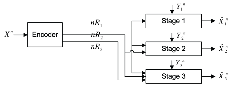
Figure 1: A three-stage successive refinement system with side informations. The side informations are degraded in the sense that $X\leftrightarrow Y_{3}\leftrightarrow Y_{2}\leftrightarrow Y_{1}$.

Let $\hat{\mathcal{X}}$ be a finite reconstruction alphabet, and let

$$\mathit{d}:\mathcal{X}\times\hat{\mathcal{X}}\rightarrow\left[0,\infty\right)$$ (2)

be a distortion measure. For simplicity, we will assume the decoders at all the stages use the same reconstruction alphabet and have the same distortion measure. The generalization to different distortion measures and reconstruction alphabets is quite simple. The per-letter distortion of a vector is defined as

$$\mathit{d}(\mbox{\boldmath$x$},\mbox{\boldmath$\hat{x}$})=\frac{1}{n}\sum_{i=1}^{n}\mathit{d}(x_{i},\hat{x}_{i}),\quad\forall\mbox{\boldmath$x$}\in\mathcal{X}^{n},\quad\mbox{\boldmath$\hat{x}$}\in\hat{\mathcal{X}}^{n}.$$ (3)

All the $\log$ function in this work is taken to be base 2.

Definition 1

An $(n,M_{1},M_{2},...,M_{N},D_{1},D_{2},...,D_{N})$ successive refinement (SR) code for source $X$ with side information $(Y_{1},Y_{2},...,Y_{N})$ consists of $N$ encoding functions $\phi_{m}$, $m=1,2,...,N$, and $N$ decoding functions $\psi_{m}$, $m=1,2,...,N$:

$$\phi_{m} : \mathcal{X}^{n}\rightarrow I_{M_{m}}$$ (4)

$$\psi_{m} : I_{M_{1}}\times I_{M_{2}}\times...\times I_{M_{m}}\times\mathcal{Y}_{m}^{n}\rightarrow\hat{\mathcal{X}^{n}},$$ (5)

where $I_{k}=\{1,2,...,k\}$, such that

$$\mbox{${\mathbb{E}}$}\mathit{d}(X^{n},\psi_{m}(\phi_{1}(X^{n}),\phi_{1}(X^{n}),...,\phi_{m}(X^{n}),Y_{m}^{n}))\leq D_{m},$$ (6)

where ${\mathbb{E}}$ is the expectation operation.

Definition 2

A rate vector $\mbox{\boldmath$R$}=(R_{1},R_{2},...,R_{N})$ is said to be $\mbox{\boldmath$D$}=(D_{1},D_{2},...,D_{N})$ achievable, if for every $\epsilon>0$ there exists for sufficient large $n$ an $(n,M_{1},M_{2},...,M_{N},D_{1}+\epsilon,D_{2}+\epsilon,...,D_{N}+\epsilon)$ code with

$$R_{m}+\epsilon\leq\frac{1}{n}\log M_{m},\quad m=1,2,...,N.$$ (7)

A three-stage example is given in Fig. 1. Denote the collection of all the $D$ achievable rate vectors as $\mathcal{R}(\mbox{\boldmath$D$})$, and this is the region to be characterized. When the side informations have arbitrary dependence among them, the problem appears to be difficult. As in [5], we consider only the case with a particularly ordered degraded side informations, which is given by the Markov condition $X\leftrightarrow Y_{N}\leftrightarrow Y_{N-1}\leftrightarrow...\leftrightarrow Y_{1}$. One of our main results is the complete characterization of this region, given in the next section.

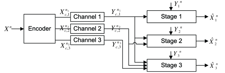
Figure 2: The corresponding source channel coding problem for the source coding system depicted in Fig. 1. .

We can further consider the case when the descriptions are transmitted over $N$ independent discrete memoryless channel (DMC) (see Fig 2). For simplicity, instead of using the more general model where the channels are cost-constrained as in [11], we only consider channels without constraints; however, such an extension can be done without much difficulty.

Definition 3

An $(n,n_{1},n_{2},...,n_{N},D_{1},D_{2},...,D_{N})$ source-channel SR (SC-SR) code for source $X$ with side information $(Y_{1},Y_{2},...,Y_{N})$ for independent channels given by $P_{Y_{c,m}|X_{c,m}}$, $m=1,2,...,N$, consists of $N$ encoding functions $\phi_{m}$, $m=1,2,...,N$, and $N$ decoding functions $\psi_{m}$, $m=1,2,...,N$:

$$\phi_{m} : \mathcal{X}^{n}\rightarrow\mathcal{X}^{n_{m}}_{c,m}$$ (8)

$$\psi_{m} : \mathcal{Y}^{n_{1}}_{c,1}\times\mathcal{Y}^{n_{2}}_{c,2}\times...\times\mathcal{Y}^{n_{m}}_{c,m}\times\mathcal{Y}_{m}^{n}\rightarrow\hat{\mathcal{X}^{n}},$$ (9)

such that

$$\mbox{${\mathbb{E}}$}\mathit{d}(X^{n},\psi_{m}(\mbox{\boldmath$Y_{c,1}$},\mbox{\boldmath$Y_{c,2}$},...,\mbox{\boldmath$Y_{c,3}$},\mbox{\boldmath$Y_{m}$}))\leq D_{m}.$$ (10)

Definition 4

A distortion vector $\mbox{\boldmath$D$}=(D_{1},D_{2},...,D_{N})$ is said to be SC-SR achievable for source $P_{XY_{1}Y_{2},...,Y_{N}}$ and channels $P_{Y_{c,m}|X_{c,m}}$, $m=1,2,...,N$, under bandwidth expansion factor $(\rho_{1},\rho_{2},...,\rho_{N})$, if for every $\epsilon>0$ there exists for sufficient large $n$ an $(n,n\rho_{1},n\rho_{2},...,n\rho_{N},D_{1}+\epsilon,D_{2}+\epsilon,...,D_{N}+\epsilon)$ SC-SR code. The achievable SC-SR distortion region $\mathcal{D}(\rho_{1},\rho_{2},...,\rho_{N})$ is the collection of all the SC-SR achievable distortion vectors under the given bandwidth expansion factors.

3 The Characterization of the Rate-distortion Region with Degraded Side Information

Define the region $\mathcal{R}^{*}(\mbox{\boldmath$D$})$ to be the set of all rate vectors $\mbox{\boldmath$R$}=(R_{1},R_{2},...,R_{N})$ for which there exists $N$ random variables $(W_{1},W_{2},...,W_{N})$ in finite alphabets $\mathcal{W}_{1},\mathcal{W}_{2},...,\mathcal{W}_{N}$ such that the following condition are satisfied.

1. $(W_{1},W_{2},...,W_{N})\leftrightarrow X\leftrightarrow Y_{N}\leftrightarrow Y_{N-1}\leftrightarrow...\leftrightarrow Y_{1}$.

2. There exist deterministic maps $f_{m}:\mathcal{W}_{m}\times\mathcal{Y}_{m}\rightarrow\hat{\mathcal{X}}$ such that

   $$\mbox{${\mathbb{E}}$}\mathit{d}(X,f_{m}(W_{m},Y_{m}))\leq D_{m},\quad 1\leq m\leq N.$$ (11)

3. The alphabet sizes satisfies

   $$|\mathcal{W}_{1}| \leq |\mathcal{X}|+2N-1$$

   $$|\mathcal{W}_{m}| \leq |\mathcal{X}|\prod_{i=1}^{m-1}|\mathcal{W}_{i}|+2N-2m-1,\quad m=2,3,...,N.$$ (12)

4. The non-negative rate vectors satisfies:

   $$\sum_{i=1}^{m}R_{i}\geq\sum_{i=1}^{m}I(X;W_{m}|W_{1},W_{2},...,W_{m-1},Y_{m}),\quad 1\leq m\leq N.$$ (13)

where we have used the convention that $W_{0}=\emptyset$, i.e., the null set.

Remark 1

Because of the conditioning on $W_{1},W_{2},...,W_{m-1}$ in the rate expressions, it is clear that the function $f_{m}(W_{m},Y_{m})$ can also be written as $f_{m}^{\prime}(W_{1},W_{2},...,W_{m},Y_{m})$ without essential difference on the definition of the region. This equivalence will be used in the explicit calculation of the rate-distortion region in Section 5 and 6. Furthermore, more structure can be built into the random variables $W_{m}$’s, such that the Markov chain holds as follows $W_{1}\leftrightarrow W_{2}\leftrightarrow...\leftrightarrow W_{N}\leftrightarrow X\leftrightarrow Y_{N}\leftrightarrow Y_{N-1}\leftrightarrow...\leftrightarrow Y_{1}$; however, such additional structure requires an increase in the cardinality of the alphabets (see discussions in [5]).

The following theorem establishes the rate-distortion region, which is one of the main results of the paper.

Theorem 1

For any discrete memoryless stochastically degraded source $X\leftrightarrow Y_{N}\leftrightarrow Y_{N-1}\leftrightarrow...\leftrightarrow Y_{1}$

$$\mathcal{R}(\mbox{\boldmath$D$})=\mathcal{R}^{*}(\mbox{\boldmath$D$}).$$ (14)

The achievability of the region is quite straightforward. The $m$-th stage codebook of overall size $2^{n(I(X;W_{m}|W_{1},W_{2},...,W_{m-1})+\epsilon_{m})}$ is generated uniform-randomly from $T_{[W_{m}|\mbox{\boldmath$w_{1}$},\mbox{\boldmath$w_{2}$},...,\mbox{\boldmath$w_{m-1}$}]\delta}^{n}$, where $T_{[W_{m}|\mbox{\boldmath$w_{1}$},\mbox{\boldmath$w_{2}$},...,\mbox{\boldmath$w_{m-1}$}]\delta}^{n}$ denotes the set of $\delta$-typical sequences given lower-hierarchy codewords $(\mbox{\boldmath$w_{1}$},\mbox{\boldmath$w_{2}$},...,\mbox{\boldmath$w_{m-1}$})$. These codewords are then placed into $2^{n(I(X;W_{m}|W_{1},W_{2},...,W_{m-1},Y_{m})+2\epsilon_{m})}$ bins using a uniform distribution. The decoder block-decodes $W_{m}$ in the $m$-th stage (using the side information), which is conditional on the lower hierarchy codewords; since the side informations are degraded, each higher hierarchy can always decode the lower-hierarchy codewords. From the above interpretation, it is seen that the proof of the achievability of the region essentially uses the hierarchy of random codes as in the proof of the two stage case in [5]. Thus we will focus on the converse part of the proof of the theorem, which is given in Appendix A.

A source-channel separation result is now stated, and the proof is given in Appendix B.

Theorem 2

For any discrete memoryless stochastically degraded source $X\leftrightarrow Y_{N}\leftrightarrow Y_{N-1}\leftrightarrow...\leftrightarrow Y_{1}$, and N independent discrete memoryless channels given by $P_{Y_{c,m}|X_{c,m}}$, $m=1,2,...,N$, the distortion vector $\mbox{\boldmath$D$}=(D_{1},D_{2},...,D_{n})$ is achievable under bandwidth expansion factors $(\rho_{1},\rho_{2},...,\rho_{N})$, if and only if there exist random variables $(W_{1},W_{2},...,W_{N})$ in finite alphabets $\mathcal{W}_{1},\mathcal{W}_{2},...,\mathcal{W}_{N}$ satisfying conditions 1), 2), 3) in the definition of $\mathcal{R}^{*}(\mbox{\boldmath$D$})$ and furthermore,

$$\sum_{i=1}^{m}\rho_{i}C_{i}\geq\sum_{i=1}^{m}I(X;W_{m}|W_{1},W_{2},...,W_{m-1},Y_{m}),\quad 1\leq m\leq N,$$ (15)

where $C_{i}$ is the channel capacity of channel $i$.

The rate region given in Theorem 1 is in a different form than the achievable region given in [5]. Here $\mathcal{R}^{*}(\mbox{\boldmath$D$})$ is given in terms of the sum-rate at each stage, including rates at the previous stages, the sufficiency of which was formally established in [12]. The achievable region in [5], denoted as $\hat{\mathcal{R}}^{*}(\mbox{\boldmath$D$})$ here, involves $(N+1)N/2$ random variables, and is given in terms of individual rate $R_{m}$ at each stage. It is provided below for ease of comparison: $\hat{\mathcal{R}}^{*}(\mbox{\boldmath$D$})$ is defined as the set of all rate vectors $(R_{1},R_{2},...,R_{N})$ for which there exists a collection of $(N+1)N/2$ random variables $\{V_{i,j},1\leq i\leq N,i\leq j\leq N\}$, where $V_{i,j}$ is taking values in a finite set $\mathcal{V}_{i,j}$, such that the following conditions are satisfied.

1. $\{V_{i,j},1\leq i\leq N,i\leq j\leq N\}\leftrightarrow X\leftrightarrow Y_{N}\leftrightarrow Y_{N-1}\leftrightarrow...\leftrightarrow Y_{1}$.

2. There exist deterministic maps $f_{m}:\mathcal{V}_{m,m}\times\mathcal{Y}_{m}\rightarrow\hat{\mathcal{X}}$ such that

   $$\mbox{${\mathbb{E}}$}\mathit{d}(X,f_{m}(V_{m,m},Y_{m}))\leq D_{m},\quad 1\leq m\leq N.$$ (16)

3. The rate vectors satisfies:

   $$R_{1} \geq I(X;V_{1,1}|Y_{1})+\sum_{k=2}^{N}I(X;V_{1,k}|V_{1,1},V_{1,2},...,V_{1,k-1},Y_{k})$$ (17)

   $$R_{m} \geq I(X;V_{m,m}|\{V_{i,j},\ 1\leq i<m,\ i\leq j\leq m\},Y_{m})$$

   $$\qquad+\sum_{k=m+1}^{N}I(X;V_{m,k}|\{V_{i,j},1\leq i\leq m,\ i\leq j\leq k-1\},Y_{k}),\quad 2\leq m\leq N.$$ (18)

It is clear that the characterization $\mathcal{R}^{*}(\mbox{\boldmath$D$})$ given in Theorem 1 is more concise. However, it can indeed be shown that these two regions are equivalent, and we establish this equivalence as a theorem.

Theorem 3

For any discrete memoryless stochastically degraded source $X\leftrightarrow Y_{N}\leftrightarrow Y_{N-1}\leftrightarrow...\leftrightarrow Y_{1}$

$$\hat{\mathcal{R}}^{*}(\mbox{\boldmath$D$})=\mathcal{R}^{*}(\mbox{\boldmath$D$})=\mathcal{R}(\mbox{\boldmath$D$}).$$ (19)

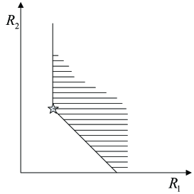
Figure 3: An example when the achievability of the two regions are equivalent, but the two regions are not the same. One region is singleton point labeled using the star, the other region is the shaded region including this singleton point.

The second equality obviously follows from Theorem 1. Theorem 3 is proved in Appendix C, which might be of interest for the following reason. In [5], a proof for a similar but different claim was given for the special case of $N=2$, which showed that the achievability of $\hat{\mathcal{R}}^{*}(\mbox{\boldmath$D$})$ and $\mathcal{R}^{*}(\mbox{\boldmath$D$})$ are equivalent. However, this does not directly imply that the two regions are equivalent; see Fig. 3 for such an example. In our proof, the fact that $\mathcal{R}^{*}(\mbox{\boldmath$D$})=\mathcal{R}(\mbox{\boldmath$D$})$ is used; and since $\hat{\mathcal{R}}^{*}(\mbox{\boldmath$D$})$ is an achievable region, we have trivially $\mathcal{R}^{*}(\mbox{\boldmath$D$})\supseteq\hat{\mathcal{R}}^{*}(\mbox{\boldmath$D$})$. However, without invoking $\mathcal{R}^{*}(\mbox{\boldmath$D$})=\mathcal{R}(\mbox{\boldmath$D$})$, it appears difficult to prove this inclusion. Interestingly, for $N=2$, it is indeed possible to prove Theorem 2 without invoking $\mathcal{R}^{*}(\mbox{\boldmath$D$})=\mathcal{R}(\mbox{\boldmath$D$})$, and this alternative proof is also included in Appendix C.

The following observation might shed some light on why a direct proof of $\hat{\mathcal{R}}^{*}(\mbox{\boldmath$D$})=\mathcal{R}(\mbox{\boldmath$D$})$ might be difficult, and it also provides the necessary intuition in proving Theorem 3. Consider the case $N=3$, the random variable $V_{1,3}$ is the information that the first stage encoded for the third stage. However, if the second stage still has to encode $V_{2,2}$ with a nonzero rate, then the encoder can not encode $V_{2,2}$ conditioned on $V_{1,3}$, since the second stage decoder will not be able to decode $V_{1,3}$. Furthermore $V_{1,3}$ does not help in the second stage decoder either. As such the encoder might as well encode $V_{1,3}$ after $V_{2,2}$ is encoded, which can then be conditioned on $V_{2,2}$ to reduce the rate. Thus the optimal scheme is to encode the first stage random variable $V_{1,1}$; if there is additional bit budget left in the first stage, then adjust and encode $V_{1,2}$ conditioned on $V_{1,1}$ until $V_{1,2}=V_{2,2}$; and if there is still additional bit budget left, then adjust and encode $V_{1,3}$ conditioned on $(V_{1,1},V_{2,2})$ until $V_{1,3}=V_{3,3}$, etc.; this process carries for each stage sequentially. Thus the majority of the $N(N+1)/2$ random variables are in fact null random variables, which reflect the change of the coding strategy at boundary points. This inherent change of encoding strategy appears to pose difficulty in proving the converse using $\hat{\mathcal{R}}^{*}(\mbox{\boldmath$D$})$.

The example in Fig. 3 can also be explained by introducing the following useful property.

Property 1

A region $\mathcal{K}$ is said to be sum-incremental, if the following is true: if $\mbox{\boldmath$R$}\in\mathcal{K}$, then for any non-negative rate vector $R^{\prime}$ that satisfies $\sum_{i=1}^{m}R_{i}^{\prime}\geq\sum_{i=1}^{m}R_{i}$ for all $1\leq m\leq N$, $\mbox{\boldmath$R^{\prime}$}\in\mathcal{K}$.

It was shown in [12] that for successive refinement coding without side information, the rate region is sum-incremental. Using the same method, it can be shown that it is also true for the rate-distortion region $\mathcal{R}(\mbox{\boldmath$D$})$ of successive refinement coding in the Wyner-Ziv setting. Intuitively, this property states that “it does not matter how you divide up the rate between layers of the (successively refining) descriptions, as long as the sum-rate of first $m$ layers is sufficiently high for each $m=1,2,...,N$” [12]: we can simply move the rate in higher stages into lower stages to form new codes. The shaded region in Fig. 3 is sum-incremental, well the singleton point labeled by the star is not. Thus the shaded region can be a valid rate-distortion region for the successive refinement problem, while the singleton point is not, though the two regions imply the same achievability result. Now notice that it is quite difficult to prove (even if not impossible) $\hat{\mathcal{R}}^{*}(\mbox{\boldmath$D$})$ is sum-incremental, which suggests it will be difficult to prove $\hat{\mathcal{R}}^{*}(\mbox{\boldmath$D$})=\mathcal{R}(\mbox{\boldmath$D$})$ directly.

4 Strictly and Generalized Successive Refinability

Extending the definition of successive refinability given in [5] to an $N$-stage system, means the following.

Definition 5

A source $X$ is said to be $N$-step successively refinable along the distortion vector $\mbox{\boldmath$D$}=(D_{1},D_{2},...,D_{N})$, with side informations $(Y_{1},Y_{2},...,Y_{N})$ if

$$(R^{*}_{X|Y_{1}}(D_{1}),R^{*}_{X|Y_{2}}(D_{2})-R^{*}_{X|Y_{1}}(D_{1}),...,R^{*}_{X|Y_{N}}(D_{N})-R^{*}_{X|Y_{N-1}}(D_{N-1}))\in\mathcal{R}(\mbox{\boldmath$D$})$$ (20)

where $R^{*}_{X|Y}(\cdot)$ denotes the Wyner-Ziv rate distortion function for source $X$ with side information $Y$ at the decoder.

This definition of successive refinability will be referred to as strictly successive refinability, for reasons that will become clear shortly. The following theorem provides the conditions for $N$-stage strictly successive refinability.

Theorem 4

A discrete memoryless stochastically degraded source $X\leftrightarrow Y_{N}\leftrightarrow Y_{N-1}\leftrightarrow...\leftrightarrow Y_{1}$ is $N$-step strictly successively refinable along distortion vector $(D_{1},D_{2},...,D_{N})$, if and only if there exist random variables $(W_{1},W_{2},...,W_{N})$ and deterministic functions $f_{m}:\mathcal{W}_{m}\times\mathcal{Y}_{m}\rightarrow\hat{\mathcal{X}}$ for $m=1,2...,N$ such that the following conditions hold:

1. $R^{*}_{X|Y_{m}}(D_{m})=I(X;W_{m}|Y_{m})$ and $\mbox{${\mathbb{E}}$}\mathit{d}(X,f_{m}(W_{m},Y_{m}))\leq D_{m}$, $1\leq m\leq N$;

2. $(W_{1},W_{2},...,W_{N})\leftrightarrow X\leftrightarrow Y_{N}\leftrightarrow Y_{N-1}\leftrightarrow...\leftrightarrow Y_{1}$;

3. $(W_{1},W_{2},...,W_{m-1})\leftrightarrow(W_{m},Y_{m})\leftrightarrow X$, $2\leq m\leq N$;

4. $I(W_{i};Y_{m}|W_{1},W_{2},...,W_{i-1},Y_{i})=0$, $1\leq i\leq m-1$, $2\leq m\leq N$.

The conditions reduce to the corresponding conditions for the two stage cases in [5]. Note that there are in fact a total of $N(N-1)/2$ equalities specified by condition 4).

Proof of Theorem 4

For the necessity, assume (20) holds. By Theorem 1, there exists random variables $(W_{1},W_{2},...,W_{N})$ and maps $f_{m}:\mathcal{W}_{m}\times\mathcal{Y}_{m}\rightarrow\hat{\mathcal{X}}$, such that $(W_{1},W_{2},...,W_{N})\leftrightarrow X\leftrightarrow Y_{N}\leftrightarrow Y_{N-1}\leftrightarrow...\leftrightarrow Y_{1}$, and since (20) holds, due to (13) we have,

$$R^{*}_{X|Y_{m}}(D_{m})\geq\sum_{i=1}^{m}I(X;W_{i}|W_{1},W_{2},...,W_{i-1},Y_{i}),\quad 1\leq m\leq N,$$ (21)

and $\mbox{${\mathbb{E}}$}\mathit{d}(X,f_{m}(W_{m},Y_{m}))\leq D_{m}$, $1\leq m\leq N$. From (21), it follows that

$$R^{*}_{X|Y_{m}}(D_{m})\geq\sum_{i=1}^{m}I(X;W_{i}|W_{1},W_{2},...,W_{i-1},Y_{i})$$

$$\stackrel{{\scriptstyle(a)}}{{=}} [I(X;W_{m}|W_{1},W_{2},...,W_{m-1},Y_{m})+\sum_{i=1}^{m-1}I(X;W_{i}|W_{1},W_{2},...,W_{i-1},Y_{i})]$$

$$+[\sum_{i=1}^{m-1}I(X;W_{i}|W_{1},W_{2},...,W_{i-1},Y_{m})-\sum_{i=1}^{m-1}I(X;W_{i}|W_{1},W_{2},...,W_{i-1},Y_{m})]$$

$$\stackrel{{\scriptstyle(b)}}{{=}} I(X;W_{1},W_{2},...,W_{m}|Y_{m})+\sum_{i=1}^{m-1}[H(W_{i}|W_{1},W_{2},...,W_{i-1},Y_{i})-H(W_{i}|W_{1},W_{2},...,W_{i-1},Y_{i},X)$$

$$-H(W_{i}|W_{1},W_{2},...,W_{i-1},Y_{m})+H(W_{i}|W_{1},W_{2},...,W_{i-1},Y_{m},X)]$$

$$\stackrel{{\scriptstyle(c)}}{{=}} I(X;W_{1},W_{2},...,W_{m}|Y_{m})+\sum_{i=1}^{m-1}[H(W_{i}|W_{1},W_{2},...,W_{i-1},Y_{i})-H(W_{i}|W_{1},W_{2},...,W_{i-1},Y_{m})]$$

$$\stackrel{{\scriptstyle(d)}}{{=}} I(X;W_{1},W_{2},...,W_{m}|Y_{m})+\sum_{i=1}^{m-1}I(W_{i};Y_{m}|W_{1},W_{2},...,W_{i-1},Y_{i})$$

$$= I(X;W_{m}|Y_{m})+I(X;W_{1},W_{2},...,W_{m-1}|Y_{m},W_{m})+\sum_{i=1}^{m-1}I(W_{i};Y_{m}|W_{1},W_{2},...,W_{i-1},Y_{i})$$

$$\geq R^{*}_{X|Y_{m}}(D_{m})+\sum_{i=1}^{m-1}I(W_{i};Y_{m}|W_{1},W_{2},...,W_{i-1},Y_{i})$$ (23)

$$\geq R^{*}_{X|Y_{m}}(D_{m})$$ (24)

where $(a)$ is by chain rule and adding and subtracting the same term, (b) follows by combining the first and third terms, $(c)$ is due to the Markov chain relationship $(W_{1},W_{2},...,W_{N})\leftrightarrow X\leftrightarrow Y_{N}\leftrightarrow Y_{N-1}\leftrightarrow...\leftrightarrow Y_{1}$; $(d)$ is also due to the same Markov chain relationship which implies we can further condition the last term in $(\ref{eqn:srcondition})$ with $Y_{i}$. Next, inequality (23) is due to the fact that $(W_{m},Y_{m})$ is sufficient to decode to a distortion $D_{m}$ while at the same time satisfying the Markov condition $W_{m}\leftrightarrow X\leftrightarrow Y_{m}$. Because the beginning and the end of this chain of inequalities are equal, all the inequalities must be equalities. For (23), the following two conditions must be true

$$I(X;W_{m}|Y_{m})=R^{*}_{X|Y_{m}}(D_{m}),\quad I(X;W_{1},W_{2},...,W_{m-1}|Y_{m},W_{m})=0$$ (25)

which implies $(W_{1},W_{2},...,W_{m-1})\leftrightarrow(W_{m},Y_{m})\leftrightarrow X$ for $2\leq m\leq N$. For (24), it must be true that for $2\leq m\leq N$

$$I(W_{i};Y_{m}|W_{1},W_{2},...,W_{i-1},Y_{i})=0,\quad 1\leq i\leq m-1.$$ (26)

This establishes the necessity. The sufficiency is of course trivial. The proof is completed. $\square$

Remark 2

: Following Remark 1 made after the definition of $\mathcal{R}^{*}(\mbox{\boldmath$D$})$, we note that if the function $f_{m}(W_{m},Y_{m})$ is indeed given instead as $f_{m}^{\prime}(W_{1},W_{2},...,W_{m},Y_{m})$, then the third condition in Theorem 4 will not appear in this set of conditions, and the first condition should be modified as: $R^{*}_{X|Y_{m}}(D_{m})=I(X;W_{1},W_{2},...,W_{m}|Y_{m})$ and $\mbox{${\mathbb{E}}$}\mathit{d}(X,f_{m}^{\prime}(W_{1},W_{2},...,W_{m},Y_{m}))\leq D_{m}$, $1\leq m\leq N$.

In order to introduce the notion of generalized successive refinability, we note that the problem considered in [6],[7] can be understood in the framework being treated as the projection of rate vector $\mathcal{R}(\mbox{\boldmath$D$})$ on the sum-rate $\sum_{i=1}^{N}R_{i}$ and ignoring the individual rate; i.e., it is a relaxed version of the current problem. Let us denote the sum-rate-distortion function to satisfy distortion constraint vector $(D_{1},D_{2},...,D_{m})$ with degraded side information $(Y_{1},Y_{2},...,Y_{m})$ as $R_{HB}(D_{1},D_{2},...,D_{m})$, which was given in [6]. Since $R_{HB}(D_{1},D_{2},...,D_{m})$ degenerates to $R^{*}_{X|Y_{m}}(D_{m})$ when all the other distortion constraints $(D_{1},D_{2},...,D_{m-1})$ are set to be infinite, it is seen that $R_{HB}(D_{1},D_{2},...,D_{m})\geq R^{*}_{X|Y_{m}}(D_{m})$. Because $R_{HB}(D_{1},D_{2},...,D_{m})$ is a lower bound for the sum-rate of $\sum_{i=1}^{m}R_{i}$, if $R_{HB}(D_{1},D_{2},...,D_{m})>R^{*}_{X|Y_{m}}(D_{m})$ for any $m\in I_{N}$, then the source is trivially not strictly successively refinable.

From the above discussion, it is seen that for a source to be strictly successively refinable, two conditions are necessary. The first is that $R_{HB}(D_{1},D_{2},...,D_{m})=R^{*}_{X|Y_{m}}(D_{m})$; and the second is that in achieving $(D_{1},D_{2},...,D_{m})$ for side information $(Y_{1},Y_{2},...,Y_{m})$, the encoding can be performed progressively without rate loss. The first condition in fact provides a simple necessary condition to check whether a source is successive refinable without directly testing the conditions in Theorem 4, which can be quite difficult because of the involvement of random variables $W_{i}$.

Theorem 5

A necessary condition for a discrete memoryless stochastically degraded source $X\leftrightarrow Y_{N}\leftrightarrow Y_{N-1}\leftrightarrow...\leftrightarrow Y_{1}$ to be $N$-step strictly successively refinable along distortion vector $(D_{1},D_{2},...,D_{N})$, is that $R_{HB}(D_{1},D_{2},...,D_{m})=R^{*}_{X|Y_{m}}(D_{m})$ for each $1\leq m\leq N$.

This condition is in fact extremely strict, and it is not satisfied for the following two familiar sources in the two stage case.

• The Gaussian source when the two side informations are not statistically identical. This example is treated in more detail in the next section.

• Doubly-symmetric binary source (DSBS) with Hamming distortion measure, when the first stage does not have side information. An explicit calculation is given in Section 6.

A natural question arises as whether the aforementioned second condition can be satisfied separately, and for this purpose the notion of generalized successively refinable with side information is defined. This notion can be used to delineate these two conditions which result in the failure of a source being successively refinable.

Definition 6

A source $X$ is said to be $N$-step generalized successively refinable with degraded side informations, i.e., $X\leftrightarrow Y_{N}\leftrightarrow Y_{N-1}\leftrightarrow...\leftrightarrow Y_{1}$, along the distortion vector $\mbox{\boldmath$D$}=(D_{1},D_{2},...,D_{N})$, if

$$(R_{HB}(D_{1}),R_{HB}(D_{1},D_{2})-R_{HB}(D_{1}),...,R_{HB}(D_{1},D_{2},...,D_{N})-R_{HB}(D_{1},D_{2},...,D_{N-1}))$$

$$\quad\in\mathcal{R}(\mbox{\boldmath$D$}).$$

The definition is limited to the degraded side information case, because $R_{HB}(D_{1},D_{2},...,D_{N})$ is known under this condition. The notion of generalized successive refinability only considers whether in order to achieve distortion $(D_{1},D_{2},...,D_{N})$ with side informations $(Y_{1},Y_{2},...,Y_{N})$, a progressive encoder is as good as an arbitrary encoder, but ignores whether $R^{*}_{X|Y_{m}}(D_{m})=R_{HB}(D_{1},D_{2},...,D_{m})$ is true.

The following theorem makes explicit the connection between strictly successive refinability and the generalized version.

Theorem 6

A source $X$ is $N$-step strictly successively refinable with degraded side information along the distortion vector $\mbox{\boldmath$D$}=(D_{1},D_{2},...,D_{N})$, if and only if it is $N$-step generalized successively refinable, and $R_{HB}(D_{1},D_{2},...,D_{m})=R^{*}_{X|Y_{m}}(D_{m})$ for each $1\leq m\leq N$.

Proof of Theorem 6

The sufficiency is trivial, and we only prove the necessity. By definition, we have

$$\mbox{\boldmath$r$}^{*}=(R^{*}_{X|Y_{1}}(D_{1}),R^{*}_{X|Y_{2}}(D_{2})-R^{*}_{X|Y_{1}}(D_{1}),...,R^{*}_{X|Y_{N}}(D_{N})-R^{*}_{X|Y_{N-1}}(D_{N-1}))\in\mathcal{R}(\mbox{\boldmath$D$}).$$ (27)

Since $\mbox{\boldmath$r$}^{*}$ is achievable, it must satisfy the following lower bound:

$$\sum_{i=1}^{m}r_{i}^{*}\geq R_{HB}(D_{1},D_{2},...,D_{m}),\quad 1\leq m\leq N.$$ (28)

Define the rate vector

$$\mbox{\boldmath$r$}=(R_{HB}(D_{1}),R_{HB}(D_{1},D_{2})-R_{HB}(D_{1}),...,R_{HB}(D_{1},D_{2},...,D_{N})-R_{HB}(D_{1},D_{2},...,D_{N-1}))$$ (29)

then it follows

$$\sum_{i=1}^{m}r_{i}=R_{HB}(D_{1},D_{2},...,D_{m})\geq R^{*}_{X|Y_{m}}(D_{m})=\sum_{i=1}^{m}r_{i}^{*}\geq R_{HB}(D_{1},D_{2},...,D_{m}),\quad 1\leq m\leq N.$$ (30)

Thus the inequalities must be equality which gives $R_{HB}(D_{1},D_{2},...,D_{m})=R^{*}_{X|Y_{m}}(D_{m})$ for $1\leq m\leq N$. The sum-incremental property of the rate-distortion region $\mathcal{R}(\mbox{\boldmath$D$})$ further implies that $\mbox{\boldmath$r$}\in\mathcal{R}(\mbox{\boldmath$D$})$, which completes the proof. $\square$

The next theorem is also straightforward as a consequence of Theorem 1 and the definition of generalized successive refinability, thus the proof is omitted.

Theorem 7

A discrete memoryless stochastically degraded source $X\leftrightarrow Y_{N}\leftrightarrow Y_{N-1}\leftrightarrow...\leftrightarrow Y_{1}$ is $N$-step generalized successively refinable if and only if there exist random variables $(W_{1},W_{2},...,W_{N})$ satisfying the conditions given for $\mathcal{R}^{*}(D_{1},D_{2},...,D_{N})$ with

$$R_{HB}(D_{1},D_{2},...,D_{m})=\sum_{i=1}^{m}I(X;W_{i}|W_{1},W_{2},...,W_{i-1},Y_{i}),\quad 1\leq m\leq N.$$ (31)

Different from strictly successive refinability with degraded side information in [5] or the conventional successive refinability without side information [2], there is no Markov condition involved. Though somewhat surprising at the first sight, it is actually straightforward, because for degraded side informations, the optimal coding scheme naturally employs a progressive order. However, an arbitrary source is not necessarily generalized successively refinable along a distortion vector (pair), because a random variable $W_{1}^{*}$ optimal for the first stage, is not necessarily optimal together with any $W_{2}$ for the first two stages. An example is that any source that is not successively refinable without side information, is not generalized successively refinable if we take both the side information $Y_{1}$ and $Y_{2}$ as constant.

With the definitions above, we will show in the next section that though Gaussian source with different but degraded side informations is not strictly successively refinable, it is indeed generalized successively refinable. The reason for it to be not strictly successively refinable is thus only due to the fact $R_{HB}(D_{1},D_{2},...,D_{j})>R^{*}_{X|Y_{j}}$ in these cases. Furthermore, we will show that the same is true for the DSBS source. Unlike the conventional successive refinability without side information, when side information is involved, many familiar sources are very likely to be not strictly successively refinable unless the side information is identical at all the stages; however, they are quite likely to be generalized successively refinable.

5 Gaussian Source with Different Side Informations

We explore the Gaussian source with mean squared error distortion measure in this section. The calculation will be focused on the two-stage system, which is sufficient for the purpose of illustrating the two kinds of successive refinability; however, it can be generalized to any finite stages. We emphasize that this derivation is not a trivial extension of the one in [6] when $Y_{1}$ is a constant, and thus more details are included in Appendix D. Though all the discussions in the previous sections are for discrete sources, the result can be generalized to the Gaussian source using the techniques in [13][14].

We first recall the result in [6] for the two stage case,

$$R_{HB}(D_{1},D_{2})=\min_{p(D_{1},D_{2})}[I(X;W_{1}|Y_{1})+I(X;W_{2}|W_{1},Y_{2})],$$ (32)

where $p(D_{1},D_{2})$ is the set of all random variable $(W_{1},W_{2})\in\mathcal{W}_{1}\times\mathcal{W}_{2}$ jointly distributed with the generic random variables $(X,Y_{1},Y_{2})$, such that the following conditions are satisfied: (1) $(W_{1},W_{2})\leftrightarrow X\leftrightarrow Y_{2}\leftrightarrow Y_{1}$ is a Markov string; (2) there exist deterministic functions $f_{1}$ and $f_{2}$ such that

$$\mbox{${\mathbb{E}}$}\mathit{d}(X,f(W_{1},Y_{1}))\leq D_{1},\quad\mbox{${\mathbb{E}}$}\mathit{d}(X,f(W_{1},W_{2},Y_{2}))\leq D_{2}.$$

The source in question is $X\sim\mathcal{N}(0,\sigma_{x}^{2})$, i.e., a zero mean normal random variable with variance $\sigma_{x}^{2}$. Let $Y_{1}=X+N_{1}+N_{2}$ and $Y_{2}=X+N_{2}$, where $N_{1}\sim\mathcal{N}(0,\sigma_{1}^{2})$, $N_{2}\sim\mathcal{N}(0,\sigma_{2}^{2})$, and $X$, $N_{1}$ and $N_{2}$ are mutually independent and Gaussian; further assume that $\sigma_{1}^{2},\sigma_{2}^{2}>0$. To facilitate the discussions, we partition the distortion regions into the following subregions, as illustrated in Fig. 4, where $D_{1}^{*}$, $D_{2}^{*}$ and $\gamma$ are defined as

$$D_{1}^{*}\stackrel{{\scriptstyle\Delta}}{{=}}\frac{\sigma_{x}^{2}(\sigma_{1}^{2}+\sigma_{2}^{2})}{\sigma_{x}^{2}+\sigma_{1}^{2}+\sigma_{2}^{2}},\quad D_{2}^{*}\stackrel{{\scriptstyle\Delta}}{{=}}\frac{\sigma_{x}^{2}\sigma_{2}^{2}}{\sigma_{x}^{2}+\sigma_{2}^{2}},\quad\gamma\stackrel{{\scriptstyle\Delta}}{{=}}\frac{\sigma_{2}^{2}}{\sigma_{1}^{2}+\sigma_{2}^{2}},$$

where it is clear that $D_{1}^{*}$ and $D_{2}^{*}$ are the variance of the best MMSE linear estimator of $X$ given $Y_{1}$ and $Y_{2}$, respectively.

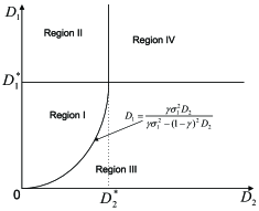
Figure 4: Partition of distortion region for the quadratic Gaussian source.

The regions can be understood as follows

• Region I: $0<D_{1}\leq D_{1}^{*}$, $0<D_{2}\leq D_{2}^{*}$ and $D_{1}\geq\frac{\gamma\sigma_{1}^{2}D_{2}}{\gamma\sigma_{1}^{2}-(1-\gamma)^{2}D_{2}}$. In this region both constraints are effective.

• Region II: $D_{1}>D_{1}^{*}$, $0<D_{2}<D_{2}^{*}$. In this region, the first stage does not have to encode, and the problem degenerates to Wyner-Ziv coding only for the second stage, i.e., $R_{1}\geq 0$ and $R_{1}+R_{2}\geq R^{*}_{X|Y_{2}}(D_{2})$.

• Region III: $D_{1}\leq D_{1}^{*}$ and $0<D_{1}<\frac{\gamma\sigma_{1}^{2}D_{2}}{\gamma\sigma_{1}^{2}-(1-\gamma)^{2}D_{2}}$. In this region, the second stage does not have to encode, and the problem degenerates to Wyner-Ziv coding only for the first stage, i.e., $R_{1}\geq R^{*}_{X|Y_{1}}(D_{1})$ and $R_{2}\geq 0$.

• Region IV: $D_{1}>D_{1}^{*}$ and $D_{2}>D_{2}^{*}$. This can be achieved with zero rate, since the side-informations are enough to satisfy the distortion constraints.

Region I is the only non-degenerate case among the four. In fact, for any distortion pairs $(D_{1},D_{2})$ in Region II, III or IV, there is a distortion pair $(D_{1}^{\prime},D_{2}^{\prime})$ on the boundary of Region I that strictly improves over $(D_{1},D_{2})$, and is achievable using the same rates; i.e., $R(D_{1},D_{2})=R(D_{1}^{\prime},D_{2}^{\prime})$, and $D_{1}\geq D_{1}^{\prime}$, $D_{2}\geq D_{2}^{\prime}$, where at least one of inequalities holds strictly. Since Region I is the only non-degenerate case, it will be our focus. For the first stage, an obvious lower bound is the Wyner-Ziv rate distortion function, which gives

$$R_{1}\geq\frac{1}{2}\log\frac{\sigma_{x}^{2}(\sigma_{1}^{2}+\sigma_{2}^{2})}{D_{1}(\sigma_{x}^{2}+\sigma_{1}^{2}+\sigma_{2}^{2})}.$$ (33)

Using $R_{HB}(D_{1},D_{2})$ as the lower bound on the sum rate, we have

$$R_{1}+R_{2}\geq R_{HB}(D_{1},D_{2})=\frac{1}{2}\log\frac{\sigma_{x}^{2}\sigma_{1}^{2}\sigma_{2}^{2}}{D_{2}(\sigma_{x}^{2}+\sigma_{1}^{2}+\sigma_{2}^{2})((1-\gamma)^{2}D_{1}+\gamma\sigma_{1}^{2})}$$ (34)

for which the rate distortion function $R_{HB}(D_{1},D_{2})$ is proved in Appendix D.

Not surprisingly, the following pair of random variables actually achieve the lower bounds on $R_{1}$ and $R_{1}+R_{2}$ simultaneously in Region I:

$$W_{1}=X+Z_{1}+Z_{2},\quad W_{2}=X+Z_{2}$$

where $Z_{1}$, $Z_{2}$ are mutually independent zero-mean Gaussian random variable, and independent of $(X,N_{1},N_{2})$, with proper choice of variances determined by $D_{1},D_{2},\sigma_{1}^{2},\sigma_{2}^{2},\sigma_{x}^{2}$. Alternatively, it is obvious that this choice of $W_{1}$ and $W_{2}$ makes all the inequalities in the lower bounding derivation satisfied with equality, thus achieves the lower bound.

From the above discussion, it is clear that this choice of $W_{1}$ and $W_{2}$ satisfies the condition of Theorem 7, and thus Gaussian source is indeed generalized successively refinable. However, in the interior of Region I, $R_{HB}(D_{1},D_{2})$ is strictly larger than $R^{*}_{X|Y_{2}}(D_{2})$, which implies Gaussian source is not successively refinable in the strict sense for these distortion pairs by Theorem 6. On the boundary between Region I and II, as well in Region II, $R_{HB}(D_{1},D_{2})=R^{*}_{X|Y_{2}}(D_{2})$, thus it is indeed successively refinable in the strict sense for these distortion pairs; however, this degenerate case is less interesting.

6 The Doubly-symmetric Binary Source

In this section we consider the following special case: $X$ is a DMS with alphabet in $\{0,1\}$, and $P(X=0)=P(X=1)=0.5$. Side information $Y_{2}=Y=X\oplus N$, where $N$ is a Bernoulli random variable independent of everything else with $P(N=1)=p<0.5$ and $\oplus$ stands for modulo 2 addition; alternatively, $Y$ can be taken as the output of a binary symmetric channel with input $X$, and crossover probability $p$. $Y_{1}$ is a constant, i.e., there is no side information at the first stage. The distortion measure is the Hamming distortion $d(x,\hat{x})=x\oplus\hat{x}$, where $\oplus$ is modulo 2 summation.

As in the Gaussian case, the function $R_{HB}(D_{1},D_{2})$ plays a significant role for this source. We digress here to give a brief review of this particular problem. The DSBS source, which is probably the simplest discrete source in the side information scenario, provided considerable insight into the Wyner-Ziv problem [4]. Somewhat surprisingly, an explicit calculation of $R_{HB}(D_{1},D_{2})$ was not found for this source. Heegard and Berger postulated a forward test channel in [6], which was later shown to be not optimal by Kerpez [8]. Kerpez provided upper and lower bounds, neither of which are tight. Fleming and Effros [9] also contributed to this problem by considering it as a rate distortion problem with mixed types of side information. An algorithm to compute the rate-distortion function numerically was further devised in [10]. However an explicit expression of the rate distortion function for this source, and more importantly the corresponding optimal forward test channel structure have not been given in the literature. In the process of considering our problem for the DSBS case, we give an explicit solution to the Heegard-Berger problem as well.

In this section we first explicitly calculate $R_{HB}(D_{1},D_{2})$, and then apply the result to the successive refinement coding case, where it will be shown that the DSBS is indeed generalized successively refinable.

6.1 $R_{HB}(D_{1},D_{2})$ for the DSBS source

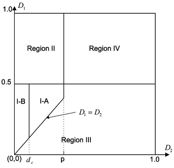
Figure 5: The four parts of the rate-distortion regions. $d_{c}$ is the critical distortion defined in [4]

As in the Gaussian case considered in Section 5, it was shown in [8] that the rate distortion region can be partitioned into four subregions, three of which are degenerate (see Fig. 5).

• Region I: $0\leq D_{1}<0.5$ and $0\leq D_{2}<\min(D_{1},p)$. In this region $R(D_{1},D_{2})$ is a function of both $D_{1}$ and $D_{2}$, and it is the only non-degenerate case;

• Region II: $D_{1}\geq 0.5$ and $0\leq D_{2}\leq p$. Here the first stage does not have to encode and therefore the problem degenerates to Wyner-Ziv encoding for the second stage.

• Region III: $0\leq D_{1}\leq 0.5$ and $D_{2}\geq\min(D_{1},p)$. Here the second stage does not have to encode and hence the problem degenerates to the rate-distortion encoding for the first stage.

• Region IV: $D_{1}>0.5$ and $D_{2}>p$. Clearly the rate is zero since the distortion constraints are trivially met.

We will need the following function from [4], defined on the domain $0\leq u\leq 1$,

$$G(u)=h(p*u)-h(u),$$

where $h(u)$ is the binary entropy function $h(u)=-u\log u-(1-u)\log(1-u)$ and $u*v$ is the binary convolution for $0\leq u,v\leq 1$ and $u*v=u(1-v)+v(1-u)$. We will be interested only in the case $0\leq p<0.5$. It was shown in [4] that $G(u)$ is (strictly) convex; furthermore, it is easy to show that $G(u)$ is symmetric about 0.5, and is monotonically decreasing for $0\leq u\leq 0.5$; the minimum of $G(u)$ is zero when $u=0.5$. It was also shown in [4] that for $0\leq D<p$

$$R^{*}_{X|Y}(D)=\min_{(\beta,\theta):0\leq\theta\leq 1,0\leq\beta\leq p,D=\theta\beta+(1-\theta)p}[\theta G(\beta)].$$ (35)

We next define the following function

$$S_{D_{1}}(\alpha,\beta,\theta,\theta_{1})=1-h(D_{1}*p)+(\theta-\theta_{1})G(\alpha)+\theta_{1}G(\beta)+(1-\theta)G(\gamma)$$

where

$$\gamma=\left\{\begin{array}[]{ll}\frac{D_{1}-(\theta-\theta_{1})(1-\alpha)-\theta_{1}\beta}{1-\theta}&\theta\neq 1\\ 0.5&\theta=1\\ \end{array}\right.$$

on the domain

$$0\leq\theta_{1}\leq\theta\leq 1,\quad 0\leq\alpha,\beta\leq p,\quad p\leq\gamma\leq 1-p.$$

Notice that $S_{D_{1}}(\cdot)$ is continuous at $\theta=1$.

The following theorem characterizes the rate distortion function $R_{HB}(D_{1},D_{2})$ in Region I.

Theorem 8

For distortion pairs $(D_{1},D_{2})$ in Region I:

$$R_{HB}(D_{1},D_{2})=\min S_{D_{1}}(\alpha,\beta,\theta,\theta_{1})\stackrel{{\scriptstyle\Delta}}{{=}}S^{*}(D_{1},D_{2}),$$

where the minimization is over the domain of $S_{D_{1}}(\alpha,\beta,\theta,\theta_{1})$, subject to the constraint

$$(\theta-\theta_{1})\alpha+\theta_{1}\beta+(1-\theta)p=D_{2}.$$

This theorem is proved in Appendix E. One notable consequence in the proof of the forward part of this theorem, is that $W_{1}$ can always be taken as the output of a BSC with crossover probability $D_{1}$ and input X. This observation is important to determine whether this source is generalized successively refinable.

The following two corollaries are useful, and are straightforward given Theorem 8, which are also proved in Appendix E. The first corollary provides a lower bound for $R_{HB}(D_{1},D_{2})$, which is easy to compute and usually tighter than the one given in [8].

Corollary 1

For distortion pairs $(D_{1},D_{2})$ in Region I:

$$R_{HB}(D_{1},D_{2})\geq 1-h(D_{1}*p)+R^{*}_{X|Y}(D_{2}).$$

Next recall the definition of the critical distortion $d_{c}$ in the Wyner-Ziv problem for the DSBS source, where

$$\frac{G(d_{c})}{d_{c}-p}=G^{\prime}(d_{c}).$$

We have the following corollary which specifies a simple forward test channel structure for the case $D_{2}\leq d_{c}$.

Corollary 2

For distortion pairs $(D_{1},D_{2})$ such that $D_{1}\leq 0.5$ and $D_{2}\leq\min(d_{c},D_{1})$ (i.e., Region I-B),

$$R_{HB}(D_{1},D_{2})=1-h(D_{1}*p)+G(D_{2}).$$

From the proof of Corollary 2, it is seen that the optimal forward test channel for this case is in fact a cascade of two BSC channels depicted in Fig. 6.

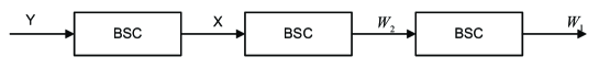
Figure 6: The optimal forward test channel in Region I-B. The crossover probability for the BSC between $X$ and $W_{2}$ is $D_{2}$, while the crossover probability $\eta$ for the BSC between $W_{2}$ and $W_{1}$ is such that $D_{2}*\eta=D_{1}$.

6.2 Successive Refinability for the DSBS Source

From Corollary 1, it is evident that $R_{HB}(D_{1},D_{2})>R^{*}_{X|Y}(D_{2})$ unless $D_{1}=0.5$, which implies that the DSBS is not strictly successively refinable; however, it is generalized successively refinable. This is true because Theorem 8 and its proof imply that $W_{1}$ can always be taken as the output of a BSC with crossover probability of $D_{2}$ and input $X$. This $W_{1}$ and the optimal $W_{2}$ clearly satisfy the condition in Theorem 7, thus the DSBS is indeed generalized successively refinable.

7 Conclusion

We provided a characterization of the rate-distortion region for the multistage successive refinement of Wyner-Ziv problem with degraded side information, which was left open in [5]. A systematical comparison with the achievable region given in [5] was provided, and the equivalence is established precisely. We also established a source-channel separation theorem when descriptions are transmitted over independent channels. Conditions for (strictly) successively refinable are accordingly derived. The notion of generalized successively refinable was introduced, in order to delineate the two obvious factors which result in the failure of a source being successively refinable. We showed that the Gaussian source with multiple side informations, as well as the doubly symmetric binary source when the first stage does not have side information, are in fact generalized successively refinable, but not strictly successively refinable. As such, their being not successively refinable is only due to the uncertainty on which side information will occur, but not the progressive encoding requirement.

Appendix A Proof of the Converse of Theorem 1

There are a total of $N$ rate constraint inequalities. We consider bounding the rate sum $\sum_{i=1}^{m}R_{i}$ for a given $m$, where $1\leq m\leq N$. Assume the existence of $(n,M_{1},M_{2},...,M_{N},D_{1},D_{2},...,D_{N})$ SR code, there exist encoding and decoding functions $\phi_{i}$ and $\psi_{i}$ for $1\leq i\leq N$. Denote $\phi_{i}(X^{n})$ as $T_{i}$. We will use the notation $T_{i}^{j}$ to denote the vector $(T_{i},T_{i+1},...,T_{j})$ when $i\leq j$; if $i>j$, we take the convention that $T_{i}^{j}$ is the empty set $\emptyset$. $(X_{1},X_{2},...,X_{n})$ will be denoted as $X$ and $(Y_{j,1},Y_{j,2},...,Y_{j,n})$ as $Y_{j}$. $\mbox{\boldmath$X$}_{k}^{-}$ will be used to denote the vector $(X_{1},X_{2},...,X_{k-1})$ and $\mbox{\boldmath$X$}_{k}^{+}$ to denote $(X_{k+1},X_{k+2},...,X_{n})$. For a collection of side informations, denote $((\mbox{\boldmath$Y_{i}$})_{k}^{+},(\mbox{\boldmath$Y_{i+1}$})_{k}^{+},...,(\mbox{\boldmath$Y_{j}$})_{k}^{+})$ as $(\mbox{\boldmath$Y_{i}^{j}$})_{k}^{+}$, and similarly for $(\mbox{\boldmath$Y_{i}^{j}$})_{k}^{-}$; they will be combined when necessary and denoted as $(\mbox{\boldmath$Y_{i}^{j}$})_{k}^{\pm}$. The subscript $k$ will be dropped when it is obvious from the context. $(Y_{i}^{j})_{k}$ is understood as the vector $(Y_{i,k},Y_{i+1,k},...,Y_{j,k})$. We will assume $m>2$ such that the quantities exist in the following proof, but it is straightforward to verify for $m=1,2$, that the derivation degenerates in the correct way.

The following chain of inequalities is straightforward

$$n\sum_{i=1}^{m}R_{i} \geq H(T_{1}^{m})$$ (37)

$$\geq H(T_{1}^{m}|\mbox{\boldmath$Y_{1}$})\stackrel{{\scriptstyle(a)}}{{=}}H(T_{1}^{m}|\mbox{\boldmath$Y_{1}$})-H(T_{1}^{m}|\mbox{\boldmath$Y_{1}$},\mbox{\boldmath$X$})$$

$$= I(\mbox{\boldmath$X$};T_{1}^{m}|\mbox{\boldmath$Y_{1}$})$$

$$= I(\mbox{\boldmath$X$};T_{1}^{m}\mbox{\boldmath$Y_{2}^{m}$}|\mbox{\boldmath$Y_{1}$})-\sum_{j=2}^{m}I(\mbox{\boldmath$X$};\mbox{\boldmath$Y_{j}$}|T_{1}^{m}\mbox{\boldmath$Y_{1}^{j-1}$})$$ (38)

$$= \sum_{k=1}^{n}[I(X_{k};T_{1}^{m}\mbox{\boldmath$Y_{2}^{m}$}|\mbox{\boldmath$Y_{1}$}\mbox{\boldmath$X$}_{k}^{-})-\sum_{j=2}^{m}I(\mbox{\boldmath$X$};Y_{j,k}|T_{1}^{m}\mbox{\boldmath$Y_{1}^{j-1}$}(\mbox{\boldmath$Y_{j}$})_{k}^{-})]$$ (39)

where $(a)$ is because the index is a function of the source, and the last two equalities follow from the chain rule for mutual information. Define the term in the outer summation of (39) as $\Gamma_{k}$, i.e.,

$$\Gamma_{k}=I(X_{k};T_{1}^{m}\mbox{\boldmath$Y_{2}^{m}$}|\mbox{\boldmath$Y_{1}$}\mbox{\boldmath$X$}_{k}^{-})-\sum_{j=2}^{m}I(\mbox{\boldmath$X$};Y_{j,k}|T_{1}^{m}\mbox{\boldmath$Y_{1}^{j-1}$}(\mbox{\boldmath$Y_{j}$})_{k}^{-})$$ (40)

For simplicity, from here on we will drop the subscript $k$ when we refer to the sequences, e.g., we will denote $\mbox{\boldmath$X$}_{k}^{-}$ by $\mbox{\boldmath$X$}^{-}$ and $(\mbox{\boldmath$Y_{j}$})_{k}^{-}$ by $\mbox{\boldmath$Y_{j}$}^{-}$. We will work primarily with $\Gamma_{k}$ until the very end of the proof. For the first term in $\Gamma_{k}$

$$I(X_{k};T_{1}^{m}\mbox{\boldmath$Y_{2}^{m}$}|\mbox{\boldmath$Y_{1}$}\mbox{\boldmath$X$}^{-})\stackrel{{\scriptstyle(a)}}{{=}}I(X_{k};T_{1}^{m}\mbox{\boldmath$Y_{2}^{m}$}{\mbox{\boldmath$Y^{\pm}_{1}$}}\mbox{\boldmath$X$}^{-}|Y_{1,k})\geq I(X_{k};T_{1}^{m}\mbox{\boldmath$Y_{2}^{m}$}{\mbox{\boldmath$Y^{\pm}_{1}$}}|Y_{1,k})$$ (41)

where (a) follows from the fact that $(X_{k},Y_{1,k})$ is independent of $(\mbox{\boldmath$X$}^{-},{\mbox{\boldmath$Y^{\pm}_{1}$}})$. Because of the Markov string $Y_{j,k}\leftrightarrow(X_{k},(Y_{1}^{j-1})_{k})\leftrightarrow(T_{1}^{m}\mbox{\boldmath$X$}^{\pm}(\mbox{\boldmath$Y_{1}^{j-1}$})^{\pm}\mbox{\boldmath$Y_{j}$}^{-})$, for each term in the negative summation in $\Gamma_{k}$, we have

$$I(\mbox{\boldmath$X$};Y_{j,k}|T_{1}^{m}\mbox{\boldmath$Y_{1}^{j-1}$}{\mbox{\boldmath$Y^{-}_{j}$}})=I(X_{k};Y_{j,k}|T_{1}^{m}\mbox{\boldmath$Y_{1}^{j-1}$}{\mbox{\boldmath$Y^{-}_{j}$}})$$ (42)

Combining (41) and (42), it follows

$$\Gamma_{k} \geq I(X_{k};T_{1}^{m}\mbox{\boldmath$Y_{2}^{m}$}{\mbox{\boldmath$Y^{\pm}_{1}$}}|Y_{1,k})-\sum_{j=2}^{m}I(X_{k};Y_{j,k}|T_{1}^{m}\mbox{\boldmath$Y_{1}^{j-1}$}{\mbox{\boldmath$Y^{-}_{j}$}})$$ (43)

Applying the chain rule for the positive term in the right hand side of (43), we have

$$I(X_{k};T_{1}^{m}\mbox{\boldmath$Y_{2}^{m}$}{\mbox{\boldmath$Y^{\pm}_{1}$}}|Y_{1,k})=I(X_{k};T_{1}^{m}\mbox{\boldmath$Y^{\pm}_{1}$}\mbox{\boldmath$Y^{-}_{2}$}|Y_{1,k})+I(X_{k};Y_{2,k}\mbox{\boldmath$Y^{+}_{2}$}\mbox{\boldmath$Y_{3}^{m}$}|T_{1}^{m}\mbox{\boldmath$Y_{1}$}\mbox{\boldmath$Y^{-}_{2}$})$$ (44)

For the second term in Eqn. (44), we have

$$I(X_{k};Y_{2,k}\mbox{\boldmath$Y^{+}_{2}$}\mbox{\boldmath$Y_{3}^{m}$}|T_{1}^{m}\mbox{\boldmath$Y_{1}$}\mbox{\boldmath$Y^{-}_{2}$})=I(X_{k};Y_{2,k}|T_{1}^{m}\mbox{\boldmath$Y_{1}$}\mbox{\boldmath$Y^{-}_{2}$})+I(X_{k};\mbox{\boldmath$Y_{2}^{+}$}\mbox{\boldmath$Y_{3}^{m}$}|T_{1}^{m}\mbox{\boldmath$Y_{1}$}\mbox{\boldmath$Y^{-}_{2}$}Y_{2,k})$$

$$=I(X_{k};Y_{2,k}|T_{1}^{m}\mbox{\boldmath$Y_{1}$}\mbox{\boldmath$Y^{-}_{2}$})+I(X_{k};\mbox{\boldmath$Y^{+}_{2}$}\mbox{\boldmath$Y^{-}_{3}$}|T_{1}^{m}\mbox{\boldmath$Y_{1}$}\mbox{\boldmath$Y^{-}_{2}$}Y_{2,k})+I(X_{k};Y_{3,k}\mbox{\boldmath$Y^{+}_{3}$}\mbox{\boldmath$Y_{4}^{m}$}|T_{1}^{m}\mbox{\boldmath$Y_{1}^{2}$}\mbox{\boldmath$Y^{-}_{3}$})$$

$$=I(X_{k};Y_{2,k}|T_{1}^{m}\mbox{\boldmath$Y_{1}$}\mbox{\boldmath$Y^{-}_{2}$})+I(X_{k};\mbox{\boldmath$Y^{+}_{2}$}\mbox{\boldmath$Y^{-}_{3}$}|T_{1}^{m}\mbox{\boldmath$Y_{1}$}\mbox{\boldmath$Y^{-}_{2}$}Y_{2,k})$$

$$\qquad\qquad\qquad+I(X_{k};Y_{3,k}|T_{1}^{m}\mbox{\boldmath$Y_{1}^{2}$}\mbox{\boldmath$Y^{-}_{3}$})+I(X_{k};\mbox{\boldmath$Y^{+}_{3}$}\mbox{\boldmath$Y_{4}^{m}$}|T_{1}^{m}\mbox{\boldmath$Y_{1}^{2}$}\mbox{\boldmath$Y^{-}_{3}$}Y_{3,k}).$$ (45)

Continuing this decomposition, it finally gives

$$I(X_{k};Y_{2,k}\mbox{\boldmath$Y^{+}_{2}$}\mbox{\boldmath$Y_{3}^{m}$}|T_{1}^{m}\mbox{\boldmath$Y_{1}$}\mbox{\boldmath$Y^{-}_{2}$})=\sum_{j=2}^{m}I(X_{k};Y_{j,k}|T_{1}^{m}\mbox{\boldmath$Y_{1}^{j-1}$}{\mbox{\boldmath$Y^{-}_{j}$}})$$

$$\qquad\qquad+\sum_{j=2}^{m-1}I(X_{k};\mbox{\boldmath$Y_{j}$}^{+}\mbox{\boldmath$Y^{-}_{j+1}$}|T_{1}^{m}\mbox{\boldmath$Y_{1}^{j-1}$}\mbox{\boldmath$Y^{-}_{j}$}Y_{j,k})+I(X_{k};\mbox{\boldmath$Y^{+}_{m}$}|T_{1}^{m}\mbox{\boldmath$Y_{1}^{m-1}$}\mbox{\boldmath$Y^{-}_{m}$}Y_{m,k}).$$ (46)

Substituting this in (44), we get

$$I(X_{k};T_{1}^{m}\mbox{\boldmath$Y_{2}^{m}$}{\mbox{\boldmath$Y^{\pm}_{1}$}}|Y_{1,k})=I(X_{k};T_{1}^{m}\mbox{\boldmath$Y^{\pm}_{1}$}\mbox{\boldmath$Y^{-}_{2}$}|Y_{1,k})+\sum_{j=2}^{m}I(X_{k};Y_{j,k}|T_{1}^{m}\mbox{\boldmath$Y_{1}^{j-1}$}{\mbox{\boldmath$Y^{-}_{j}$}})$$

$$\quad\qquad\qquad+\sum_{j=2}^{m-1}I(X_{k};\mbox{\boldmath$Y_{j}$}^{+}\mbox{\boldmath$Y^{-}_{j+1}$}|T_{1}^{m}\mbox{\boldmath$Y_{1}^{j-1}$}\mbox{\boldmath$Y^{-}_{j}$}Y_{j,k})+I(X_{k};\mbox{\boldmath$Y^{+}_{m}$}|T_{1}^{m}\mbox{\boldmath$Y_{1}^{m-1}$}\mbox{\boldmath$Y^{-}_{m}$}Y_{m,k}).$$ (47)

Therefore, substituting (47) into (43) we see that the negative term in (43) cancels out the second term on the RHS of (47), which gives

$$\Gamma_{k}\geq I(X_{k};T_{1}^{m}\mbox{\boldmath$Y_{1}$}^{\pm}\mbox{\boldmath$Y^{-}_{2}$}|Y_{1,k})$$

$$\quad\quad\quad+\sum_{j=2}^{m-1}I(X_{k};\mbox{\boldmath$Y^{+}_{j}$}\mbox{\boldmath$Y^{-}_{j+1}$}|T_{1}^{m}\mbox{\boldmath$Y_{1}^{j-1}$}\mbox{\boldmath$Y^{-}_{j}$}Y_{j,k})+I(X_{k};\mbox{\boldmath$Y^{+}_{m}$}|T_{1}^{m}\mbox{\boldmath$Y_{1}^{m-1}$}\mbox{\boldmath$Y^{-}_{m}$}Y_{m,k}).$$ (48)

For the first term in (48), we have

$$I(X_{k};T_{1}^{m}\mbox{\boldmath$Y^{\pm}_{1}$}\mbox{\boldmath$Y^{-}_{2}$}|Y_{1,k})=I(X_{k};T_{1}\mbox{\boldmath$Y^{\pm}_{1}$}|Y_{1,k})+I(X_{k};T_{2}^{m}\mbox{\boldmath$Y^{-}_{2}$}|T_{1}\mbox{\boldmath$Y_{1}$}).$$ (49)

We claim that

$$I(X_{k};T_{2}^{m}\mbox{\boldmath$Y^{-}_{2}$}|T_{1}\mbox{\boldmath$Y_{1}$})\geq I(X_{k};T_{2}^{m}\mbox{\boldmath$Y^{-}_{2}$}|T_{1}\mbox{\boldmath$Y_{1}$}Y_{2,k})$$ (50)

and more generally for $2\leq j\leq m$

$$I(X_{k};T_{j}^{m}\mbox{\boldmath$Y^{-}_{j}$}|T_{1}^{j-1}\mbox{\boldmath$Y_{1}^{j-1}$})\geq I(X_{k};T_{j}^{m}\mbox{\boldmath$Y^{-}_{j}$}|T_{1}^{j-1}\mbox{\boldmath$Y_{1}^{j-1}$}Y_{j,k})$$ (51)

which can be justified as follows

$$I(X_{k};T_{j}^{m}\mbox{\boldmath$Y^{-}_{j}$}|T_{1}^{j-1}\mbox{\boldmath$Y_{1}^{j-1}$})-I(X_{k};T_{j}^{m}\mbox{\boldmath$Y^{-}_{j}$}|T_{1}^{j-1}\mbox{\boldmath$Y_{1}^{j-1}$}Y_{j,k})$$ (52)

$$= H(X_{k}|T_{1}^{j-1}\mbox{\boldmath$Y_{1}^{j-1}$})-H(X_{k}|T_{1}^{m}\mbox{\boldmath$Y_{1}^{j-1}$}\mbox{\boldmath$Y^{-}_{j}$})$$

$$\qquad\qquad\qquad-H(X_{k}|T_{1}^{j-1}\mbox{\boldmath$Y_{1}^{j-1}$}Y_{j,k})+H(X_{k}|T_{1}^{m}\mbox{\boldmath$Y_{1}^{j-1}$}\mbox{\boldmath$Y^{-}_{j}$}Y_{j,k})$$

$$= I(X_{k};Y_{j,k}|T_{1}^{j-1}\mbox{\boldmath$Y_{1}^{j-1}$})-I(X_{k};Y_{j,k}|T_{1}^{m}\mbox{\boldmath$Y^{-}_{j}$}\mbox{\boldmath$Y_{1}^{j-1}$})$$

$$= H(Y_{j,k}|T_{1}^{j-1}\mbox{\boldmath$Y_{1}^{j-1}$})-H(Y_{j,k}|X_{k}T_{1}^{j-1}\mbox{\boldmath$Y_{1}^{j-1}$})$$

$$\qquad\qquad\qquad-H(Y_{j,k}|T_{1}^{m}\mbox{\boldmath$Y^{-}_{j}$}\mbox{\boldmath$Y_{1}^{j-1}$})+H(Y_{j,k}|X_{k}T_{1}^{m}\mbox{\boldmath$Y^{-}_{j}$}\mbox{\boldmath$Y_{1}^{j-1}$})$$

$$\stackrel{{\scriptstyle(a)}}{{=}} I(Y_{j,k};T_{j}^{m}\mbox{\boldmath$Y^{-}_{j}$}|T_{1}^{j-1}\mbox{\boldmath$Y_{1}^{j-1}$})\geq 0$$

where (a) is due to the Markov condition $Y_{j,k}\leftrightarrow(X_{k},(Y_{1}^{j-1})_{k})\leftrightarrow(T_{1}^{m}\mbox{\boldmath$Y^{-}_{j}$}(\mbox{\boldmath$Y_{1}^{j-1}$})^{\pm}\mbox{\boldmath$X$}^{\pm})$ implies the reduced Markov condition $Y_{j,k}\leftrightarrow(X_{k},(Y_{1}^{j-1})_{k})\leftrightarrow(T_{1}^{m}\mbox{\boldmath$Y^{-}_{j}$}(\mbox{\boldmath$Y_{1}^{j-1}$})^{\pm})$. Assume for now $m>2$, and consider the following summation of the second term in (49) and the second term in (48)

$$I(X_{k};T_{2}^{m}\mbox{\boldmath$Y^{-}_{2}$}|T_{1}\mbox{\boldmath$Y_{1}$})+\sum_{j=2}^{m-1}I(X_{k};\mbox{\boldmath$Y^{+}_{j}$}\mbox{\boldmath$Y^{-}_{j+1}$}|T_{1}^{m}\mbox{\boldmath$Y_{1}^{j-1}$}\mbox{\boldmath$Y^{-}_{j}$}Y_{j,k})$$

$$\stackrel{{\scriptstyle(a)}}{{\geq}} I(X_{k};T_{2}^{m}\mbox{\boldmath$Y^{-}_{2}$}|T_{1}\mbox{\boldmath$Y_{1}$}Y_{2,k})+\sum_{j=2}^{m-1}I(X_{k};\mbox{\boldmath$Y^{+}_{j}$}\mbox{\boldmath$Y^{-}_{j+1}$}|T_{1}^{m}\mbox{\boldmath$Y_{1}^{j-1}$}\mbox{\boldmath$Y^{-}_{j}$}Y_{j,k})$$

$$= I(X_{k};T_{2}^{m}\mbox{\boldmath$Y^{-}_{2}$}|T_{1}\mbox{\boldmath$Y_{1}$}Y_{2,k})+I(X_{k};\mbox{\boldmath$Y_{2}$}^{+}\mbox{\boldmath$Y^{-}_{3}$}|T_{1}^{m}\mbox{\boldmath$Y_{1}$}\mbox{\boldmath$Y^{-}_{2}$}Y_{2,k})$$

$$\qquad\qquad\qquad\qquad\qquad\qquad\qquad\qquad\qquad+\sum_{j=3}^{m-1}I(X_{k};\mbox{\boldmath$Y^{+}_{j}$}\mbox{\boldmath$Y^{-}_{j+1}$}|T_{1}^{m}\mbox{\boldmath$Y_{1}^{j-1}$}\mbox{\boldmath$Y^{-}_{j}$}Y_{j,k})$$

$$\stackrel{{\scriptstyle(b)}}{{=}} I(X_{k};T_{2}^{m}\mbox{\boldmath$Y_{2}$}^{\pm}\mbox{\boldmath$Y^{-}_{3}$}|T_{1}\mbox{\boldmath$Y_{1}$}Y_{2,k})+\sum_{j=3}^{m-1}I(X_{k};\mbox{\boldmath$Y_{j}$}^{+}\mbox{\boldmath$Y^{-}_{j+1}$}|T_{1}^{m}\mbox{\boldmath$Y_{1}^{j-1}$}\mbox{\boldmath$Y^{-}_{j}$}Y_{j,k})$$

$$= I(X_{k};T_{2}\mbox{\boldmath$Y_{2}$}^{\pm}|T_{1}\mbox{\boldmath$Y_{1}$}Y_{2,k})+I(X_{k};T_{3}^{m}\mbox{\boldmath$Y^{-}_{3}$}|T_{1}^{2}\mbox{\boldmath$Y_{1}^{2}$})+\sum_{j=3}^{m-1}I(X_{k};\mbox{\boldmath$Y^{+}_{j}$}\mbox{\boldmath$Y^{-}_{j+1}$}|T_{1}^{m}\mbox{\boldmath$Y_{1}^{j-1}$}\mbox{\boldmath$Y^{-}_{j}$}Y_{j,k}),$$

where $(a)$ follows because of (51) and $(b)$ follows due to chain rule. Notice for the second term in (LABEL:eqn:h5), we can again apply inequality (51), and continue sequentially along this way, which finally gives

$$I(X_{k};T_{2}^{m}\mbox{\boldmath$Y^{-}_{2}$}|T_{1}\mbox{\boldmath$Y_{1}$})+\sum_{j=2}^{m-1}I(X_{k};\mbox{\boldmath$Y^{+}_{j}$}\mbox{\boldmath$Y^{-}_{j+1}$}|T_{1}^{m}\mbox{\boldmath$Y_{1}^{j-1}$}\mbox{\boldmath$Y^{-}_{j}$}Y_{j,k})$$

$$\qquad\geq\sum_{j=2}^{m-1}I(X_{k};T_{j}\mbox{\boldmath$Y^{\pm}_{j}$}|T_{1}^{j-1}\mbox{\boldmath$Y_{1}^{j-1}$}Y_{j,k})+I(X_{k};T_{m}\mbox{\boldmath$Y^{-}_{m}$}|T_{1}^{m-1}\mbox{\boldmath$Y_{1}^{m-1}$})$$ (54)

Combining (48), (49) and (54) gives

$$\Gamma_{k} \geq I(X_{k};T_{1}\mbox{\boldmath$Y^{\pm}_{1}$}|Y_{1,k})+\sum_{j=2}^{m-1}I(X_{k};T_{j}\mbox{\boldmath$Y^{\pm}_{j}$}|T_{1}^{j-1}\mbox{\boldmath$Y_{1}^{j-1}$}Y_{j,k})$$ (55)

$$+I(X_{k};T_{m}\mbox{\boldmath$Y^{-}_{m}$}|T_{1}^{m-1}\mbox{\boldmath$Y_{1}^{m-1}$})+I(X_{k};\mbox{\boldmath$Y^{+}_{m}$}|T_{1}^{m}\mbox{\boldmath$Y_{1}^{m-1}$}\mbox{\boldmath$Y^{-}_{m}$}Y_{m,k})$$

$$\geq \sum_{j=1}^{m}I(X_{k};T_{j}\mbox{\boldmath$Y^{\pm}_{j}$}|T_{1}^{j-1}\mbox{\boldmath$Y_{1}^{j-1}$}Y_{j,k}).$$ (56)

where inequality (51) is applied on the third term in (55). It is straightforward to verify that inequality (56) is still valid if $m=1$ or $m=2$, when the proper convention of empty set is taken.

In (56), the conditioning on $(Y_{1}^{j-1})_{k}$ has to be removed to reach the desired form, which can indeed be done due to the degradedness of the side informations. More precisely, for $2\leq j\leq m$

$$I(X_{k};T_{j}\mbox{\boldmath$Y^{\pm}_{j}$}|T_{1}^{j-1}\mbox{\boldmath$Y_{1}^{j-1}$}Y_{j,k})-I(X_{k};T_{j}\mbox{\boldmath$Y^{\pm}_{j}$}|T_{1}^{j-1}(\mbox{\boldmath$Y_{1}^{j-1}$})^{\pm}Y_{j,k})$$ (57)

$$= H(X_{k}|T_{1}^{j-1}\mbox{\boldmath$Y_{1}^{j-1}$}Y_{j,k})-H(X_{k}|T_{1}^{j}\mbox{\boldmath$Y_{1}^{j}$})-H(X_{k}|T_{1}^{j-1}(\mbox{\boldmath$Y_{1}^{j-1}$})^{\pm}Y_{j,k})+H(X_{k}|T_{1}^{j}(\mbox{\boldmath$Y_{1}^{j}$})^{\pm}Y_{j,k})$$

$$= -I(X_{k};(Y_{1}^{j-1})_{k}|T_{1}^{j-1}(\mbox{\boldmath$Y_{1}^{j-1}$})^{\pm}Y_{j,k})+I(X_{k};(Y_{1}^{j-1})_{k}|T_{1}^{j}(\mbox{\boldmath$Y_{1}^{j}$})^{\pm}Y_{j,k})=0$$

where in fact both the terms in the (57) are zero, due to the Markov condition $(Y_{1}^{j-1})_{k}\leftrightarrow Y_{j,k}\leftrightarrow(\mbox{\boldmath$X$}T_{1}^{m}(\mbox{\boldmath$Y_{1}^{m}$})^{\pm})$ implies the reduced Markov condition $(Y_{1}^{j-1})_{k}\leftrightarrow Y_{j,k}\leftrightarrow(X_{k}T_{1}^{j}(\mbox{\boldmath$Y_{1}^{j}$})^{\pm})$. Thus we reach the form

$$\Gamma_{k} \geq \sum_{j=1}^{m}I(X_{k};T_{j}\mbox{\boldmath$Y_{j}$}^{\pm}|T_{1}^{j-1}(\mbox{\boldmath$Y_{1}^{j-1}$})^{\pm}Y_{j,k})=\sum_{j=1}^{m}I(X_{k};T_{1}^{j}\mbox{\boldmath$Y_{j}$}^{\pm}|T_{1}^{j-1}(\mbox{\boldmath$Y_{1}^{j-1}$})^{\pm}Y_{j,k}).$$ (58)

Define $W_{j,k}=(T_{1}^{j},(\mbox{\boldmath$Y$}_{j})_{k}^{\pm})$ and by substituting (58) into (39) we have for $1\leq m\leq N$,

$$n\sum_{i=1}^{m}R_{i}\geq\sum_{k=1}^{n}\sum_{j=1}^{m}I(X_{k};W_{j,k}|(W_{1}^{j-1})_{k},Y_{j,k})$$ (59)

Therefore the Markov condition $(W_{1,k},W_{2,k},...,W_{N,k})\leftrightarrow X_{k}\leftrightarrow Y_{N,k}\leftrightarrow Y_{N-1,k}\leftrightarrow...\leftrightarrow Y_{1,k}$ is true. Next introduce the time sharing random variable $Q$, which is independent of the multisource, and uniformly distributed over $I_{n}$. Define $W_{j}=(W_{j,Q},Q)$. The existence of function $f_{j}$ follows by defining

$$f_{j}(W_{j},Y_{j})=\psi_{j,Q}(\phi_{1}(\mbox{\boldmath$X$}),\phi_{2}(\mbox{\boldmath$X$}),...,\phi_{j}(\mbox{\boldmath$X$}),\mbox{\boldmath$\mbox{\boldmath$Y_{j}$}$})$$ (60)

because $W_{j}$ includes $T_{1}^{j}\mbox{\boldmath$Y_{j}$}^{\pm}$, which leads to the fulfillment of the distortion constraint

$$\mbox{${\mathbb{E}}$}\mathit{d}(X,f_{j}(W_{j},Y_{j}))=\frac{1}{n}\sum_{i=1}^{n}\mbox{${\mathbb{E}}$}\mathit{d}(X_{i},\psi_{j,i}(\phi_{1}(\mbox{\boldmath$X$}),\phi_{2}(\mbox{\boldmath$X$}),...,\phi_{j}(\mbox{\boldmath$X$}),\mbox{\boldmath$Y_{j}$}))\leq D_{j},\quad 1\leq j\leq N$$

and the Markov condition $(W_{1},W_{2},...,W_{N})\leftrightarrow X\leftrightarrow Y_{N}\leftrightarrow Y_{N-1}\leftrightarrow...\leftrightarrow Y_{1}$ is still true. It only remains to show the bound (59) can be writen in single letter form in $W_{j}$, but this is straightforward following the approach on pg. 435 of [15] (see also [5]). The bounds on the alphabet size is by applying conventional argument (see [16]). This completes the proof. $\square$

Appendix B Proof of Theorem 2

The forward part is trivially implied by Theorem 1 and the conventional channel coding theorem, and thus we only give an outline of the converse part.

By Lemma 8.9.2 in [15], we have

$$n\sum_{i=1}^{m}\rho_{i}C_{i}\geq\sum_{i=1}^{m}I(X^{n_{i}}_{c,i};Y^{n_{i}}_{c,i})$$ (62)

where $n_{i}=n\rho_{i}$, and $\rho_{i}$ is the number of channel use per source symbol for the $i$-th channel. Notice that

$$I(X^{n_{1}}_{c,1}X^{n_{2}}_{c,2},...,X^{n_{m}}_{c,m};Y^{n_{1}}_{c,1}Y^{n_{2}}_{c,2},...,Y^{n_{m}}_{c,m})$$ (63)

$$\stackrel{{\scriptstyle(a)}}{{=}} I(X^{n_{1}}_{c,1}X^{n_{2}}_{c,2},...,X^{n_{m}}_{c,m};Y^{n_{1}}_{c,1})+I(X^{n_{1}}_{c,1}X^{n_{2}}_{c,2},...,X^{n_{m}}_{c,m};Y^{n_{2}}_{c,2}Y^{n_{3}}_{c,3},...,Y^{n_{m}}_{c,m}|Y^{n_{1}}_{c,1})$$

$$\stackrel{{\scriptstyle(b)}}{{=}} I(X^{n_{1}}_{c,1};Y^{n_{1}}_{c,1})+I(X^{n_{1}}_{c,1}X^{n_{2}}_{c,2},...,X^{n_{m}}_{c,m};Y^{n_{2}}_{c,2}Y^{n_{3}}_{c,3},...,Y^{n_{m}}_{c,m}|Y^{n_{1}}_{c,1})$$

$$= I(X^{n_{1}}_{c,1};Y^{n_{1}}_{c,1})+H(Y^{n_{2}}_{c,2}Y^{n_{3}}_{c,3},...,Y^{n_{m}}_{c,m}|Y^{n_{1}}_{c,1})-H(Y^{n_{2}}_{c,2}Y^{n_{3}}_{c,3},...,Y^{n_{m}}_{c,m}|Y^{n_{1}}_{c,1}X^{n_{1}}_{c,1}X^{n_{2}}_{c,2},...,X^{n_{m}}_{c,m})$$

$$\stackrel{{\scriptstyle(c)}}{{=}} I(X^{n_{1}}_{c,1};Y^{n_{1}}_{c,1})+H(Y^{n_{2}}_{c,2}Y^{n_{3}}_{c,3},...,Y^{n_{m}}_{c,m}|Y^{n_{1}}_{c,1})-H(Y^{n_{2}}_{c,2}Y^{n_{3}}_{c,3},...,Y^{n_{m}}_{c,m}|X^{n_{2}}_{c,2},...,X^{n_{m}}_{c,m})$$

$$\stackrel{{\scriptstyle(d)}}{{\leq}} I(X^{n_{1}}_{c,1};Y^{n_{1}}_{c,1})+H(Y^{n_{2}}_{c,2}Y^{n_{3}}_{c,3},...,Y^{n_{m}}_{c,m})-H(Y^{n_{2}}_{c,2}Y^{n_{3}}_{c,3},...,Y^{n_{m}}_{c,m}|X^{n_{2}}_{c,2},...,X^{n_{m}}_{c,m})$$

$$= I(X^{n_{1}}_{c,1};Y^{n_{1}}_{c,1})+I(Y^{n_{2}}_{c,2}Y^{n_{3}}_{c,3},...,Y^{n_{m}}_{c,m};X^{n_{2}}_{c,2},...,X^{n_{m}}_{c,m})$$

where (a) is by chain rule, and (b) and (c) are because the channels are independent, i.e.,

$$P_{Y_{c,1}Y_{c,2},...,Y_{c,m}|X_{c,1}X_{c,2},...,X_{c,m}}=P_{Y_{c,1}|X_{c,1}}P_{Y_{c,2}|X_{c,2}}...P_{Y_{c,m}|X_{c,m}}$$ (64)

which implies the Markov conditions $\{X_{c,j}\}_{j\neq i}\leftrightarrow X_{c,i}\leftrightarrow Y_{c,i}$ and $\{Y_{c,j}\}_{j\neq i}\leftrightarrow\{X_{c,j}\}_{j\neq i}\leftrightarrow(X_{c,i},Y_{c,i})$; (d) is because conditioning reduces entropy.

Continue this decomposition and combine it with (62), we have

$$n\sum_{i=1}^{m}\rho_{i}C_{i} \geq \sum_{i=1}^{m}I(X^{n_{i}}_{c,i};Y^{n_{i}}_{c,i})\geq I(X^{n_{1}}_{c,1}X^{n_{2}}_{c,2},...,X^{n_{m}}_{c,m};Y^{n_{1}}_{c,1}Y^{n_{2}}_{c,2},...,Y^{n_{m}}_{c,m})$$ (65)

$$\stackrel{{\scriptstyle(a)}}{{\geq}} I(X^{n};Y^{n_{1}}_{c,1}Y^{n_{2}}_{c,2},...,Y^{n_{m}}_{c,m})$$

$$\stackrel{{\scriptstyle(b)}}{{=}} I(X^{n}Y_{1}^{n};Y^{n_{1}}_{c,1}Y^{n_{2}}_{c,2},...,Y^{n_{m}}_{c,m})$$

$$= I(Y_{1}^{n};Y^{n_{1}}_{c,1}Y^{n_{2}}_{c,2},...,Y^{n_{m}}_{c,m})+I(X^{n};Y^{n_{1}}_{c,1}Y^{n_{2}}_{c,2},...,Y^{n_{m}}_{c,m}|Y_{1}^{n})$$

$$\geq I(X^{n};Y^{n_{1}}_{c,1}Y^{n_{2}}_{c,2},...,Y^{n_{m}}_{c,m}|Y_{1}^{n})$$

where (a) is due to data processing inequality, and (b) because the Markov chain $Y_{1}\leftrightarrow X\leftrightarrow Y_{c,i}$. At this point the similarity between (65) and (37) is quite clear. Using the same steps as in the derivation as in the proof of Theorem 1, the converse of Theorem 2 is proved. $\square$

Appendix C Proof of Theorem 3

We first prove for the special case $N=2$ without invoking Theorem 1 that $\mathcal{R}^{*}(\mbox{\boldmath$D$})=\mathcal{R}(\mbox{\boldmath$D$})$. The proof of Theorem 3 then follows from invoking Theorem 1 for one direction and extending the proof of $N=2$ for the other direction.

Proof for the case of $N=2$

We first prove that $\hat{\mathcal{R}}_{2}^{*}(\mbox{\boldmath$D$})\subseteq\mathcal{R}_{2}^{*}(\mbox{\boldmath$D$})$, where the subscript 2 stands for $N=2$. For an arbitrary rate pair $(r_{1},r_{2})\in\hat{\mathcal{R}}_{2}^{*}(D_{1},D_{2})$, there exist $3$ random variables $V_{1,1},V_{1,2}$ and $V_{2,2}$, and the corresponding functions $f_{1}(V_{1,1},Y_{1})$ and $f_{2}(V_{2,2},Y_{2})$, such that

$$r_{1} \geq I(X;V_{1,1}|Y_{1})+I(X;V_{1,2}|V_{1,1},Y_{2})$$ (66)

$$r_{2} \geq I(X;V_{2,2}|V_{1,1},V_{1,2},Y_{2})$$ (67)

and the distortion constraints are satisfied. Inequalities (66) and (67) imply that

$$r_{1} \geq I(X;V_{1,1}|Y_{1})$$

$$r_{1}+r_{2} \geq I(X;V_{1,1}|Y_{1})+I(X;V_{1,2}|V_{1,1},Y_{2})+I(X;V_{2,2}|V_{1,1},V_{1,2},Y_{2})$$

$$= I(X;V_{1,1}|Y_{1})+I(X;V_{1,2},V_{2,2}|V_{1,1},Y_{2})$$

Now define $W_{1}=V_{1,1}$ and $W_{2}=(V_{1,1},V_{1,2})$, and it follows that

$$r_{1} \geq I(X;W_{1}|Y_{1})$$

$$r_{1}+r_{2} \geq I(X;W_{1}|Y_{1})+I(X;W_{2}|W_{1},Y_{2})$$

and $(W_{1},W_{2})$ is a pair of random variables satisfying the condition for $\mathcal{R}_{2}^{*}(D_{1},D_{2})$ and thus $(r_{1},r_{2})\in\mathcal{R}_{2}^{*}(D_{1},D_{2})$, which shows that $\hat{\mathcal{R}}_{2}^{*}(\mbox{\boldmath$D$})\subseteq\mathcal{R}_{2}^{*}(\mbox{\boldmath$D$})$ since trivially the distortion constraints are also met.

To prove the other direction, i.e., $\hat{\mathcal{R}}_{2}^{*}(D_{1},D_{2})\supseteq\mathcal{R}_{2}^{*}(D_{1},D_{2})$, assume $(r_{1},r_{2})\in\mathcal{R}_{2}^{*}(D_{1},D_{2})$. There exist random variables $W_{1}$ and $W_{2}$, and two corresponding functions $f_{1}(W_{1},Y_{1})$ and $f_{2}(W_{2},Y_{2})$, such that

$$r_{1} \geq I(X;W_{1}|Y_{1})$$ (68)

$$r_{1}+r_{2} \geq I(X;W_{1}|Y_{1})+I(X;W_{2}|W_{1},Y_{2})$$ (69)

and the distortion constraints are met. Let $\Delta r_{1}=r_{1}-I(X;W_{1}|Y_{1})$. We claim that for any $0\leq\Delta r_{1}\leq I(X;W_{2}|W_{1},Y_{2})$, there exists a random variable $V$, such that

$$\Delta r_{1}=I(X;V|W_{1},Y_{2})$$ (70)

$$I(X;V|W_{1},Y_{2})+I(X;W_{2}|W_{1},V,Y_{2})=I(X;W_{2}|W_{1},Y_{2}).$$ (71)

There are many ways to construct $V$, for example we can construct $V=(W_{2}(J),J)$, where $J$ is a Bernoulli random variable independent of everything else with $p(J=1)=u$; when $J=1$, $W_{2}(J)=W_{2}$ and $W_{2}(J)$ is a fixed constant otherwise; $I(X;V|W_{1},Y_{2})$ can be any real value in the interval $[0,I(X;W_{2}|W_{1},Y_{2})]$ by choosing $u$ appropriately. For a more thorough treatment on this topic in the context of rate splitting in multiple access channel, see [17]. It follows that for this case

$$r_{1} = I(X;W_{1}|Y_{1})+I(X;V|W_{1},Y_{2})$$ (72)

$$r_{2} \geq I(X;W_{1}|Y_{1})+I(X;W_{2}|W_{1},Y_{2})-r_{1}$$ (73)

$$= I(X;W_{2}|W_{1},V,Y).$$

Now define $V_{1,1}=W_{1}$, $V_{1,2}=V$ and $V_{2,2}=W_{2}$. The random variables $(V_{1,1},V_{1,2},V_{2,2})$ clearly satisfy the definition given for $\hat{\mathcal{R}}^{*}(D_{1},D_{2})$, and thus $(r_{1},r_{2})\in\hat{\mathcal{R}}^{*}(D_{1},D_{2})$ for this case. On the other hand, if $\Delta r_{1}\geq I(X;W_{2}|W_{1},Y_{2})$, then defines $V_{1,1}=W_{1}$, $V_{1,2}=W_{2}$ and $V_{2,2}=W_{2}$. The non-negativity condition $r_{2}\geq 0$ implies $r_{2}\geq I(X;V_{2,2}|V_{1,1},V_{1,2},Y_{2})$. Since the reconstruction functions $f_{1}(W_{1},Y_{1})=f_{1}(V_{1,1},Y_{1})$ and $f_{2}(W_{2},Y_{2})=f_{2}(V_{2,2},Y_{2})$ satisfy the distortion constraints, the proof is completed. $\square$

Proof of Theorem 3

Since $\hat{\mathcal{R}}^{*}(\mbox{\boldmath$D$})$ is an achievable region, we have trivially $\hat{\mathcal{R}}^{*}(\mbox{\boldmath$D$})\subseteq\mathcal{R}(\mbox{\boldmath$D$})=\mathcal{R}^{*}(\mbox{\boldmath$D$})$ due to Theorem 1. For the inclusion of the other direction, the proof for the case $N=2$ can clearly be extended straightforwardly, by sequentially constructing random variable corresponding to $\{V_{i,j}\},j\geq i$. This completes the proof for Theorem 3. $\square$

Appendix D Lower Bound on the Sum-rate for the Gaussian Source

To lower bound the sum-rate to achieve $(D_{1},D_{2})$ with side information $(Y_{1},Y_{2})$, consider the following quantity,

$$I(X;W_{1}|Y_{1})+I(X;W_{2}|W_{1},Y_{2})$$ (74)

$$= H(X|Y_{1})-H(X|W_{1},Y_{1})+H(X|W_{1},Y_{2})-H(X|W_{1},W_{2},Y_{2})$$

$$\stackrel{{\scriptstyle(a)}}{{=}} H(X|Y_{1})-H(X|W_{1},W_{2},Y_{2})-I(X;Y_{2}|W_{1},Y_{1})$$

$$\stackrel{{\scriptstyle(b)}}{{=}} H(X|Y_{1})-H(X|W_{1},W_{2},Y_{2})-H(Y_{2}|W_{1},Y_{1})+H(Y_{2}|X,Y_{1})$$ (75)

where we can see $(a)$ follows since $I(W_{1},X;Y_{1}|Y_{2})=I(W_{1};Y_{1}|Y_{2})+I(X;Y_{1}|W_{1},Y_{2})=0$ due to the Markov condition $W_{1}\leftrightarrow X\leftrightarrow Y_{2}\leftrightarrow Y_{1}$, which implies that $I(X;Y_{1}|W_{1},Y_{2})=H(X|W_{1},Y_{2})-H(X|W_{1},Y_{2},Y_{1})=0$. In an identical manner $(b)$ is due to, $I(W_{1};Y_{2}|X,Y_{1})=H(Y_{2}|X,Y_{1})-H(Y_{2}|X,Y_{1},W_{1})=0$. The quantities $H(X|Y_{1})$ and $H(Y_{2}|X,Y_{1})$ are only dependent on the multi-source. We bound the second term in (75) as follows

$$H(X|W_{1},W_{2},Y_{2}) = H(X-\mbox{${\mathbb{E}}$}(X|W_{1},W_{2},Y_{2})|W_{1},W_{2},Y_{2})$$ (76)

$$\leq H(X-\mbox{${\mathbb{E}}$}(X|W_{1},W_{2},Y_{2}))$$

$$\leq H(\mathcal{N}(0,\mbox{${\mathbb{E}}$}(X-\mbox{${\mathbb{E}}$}(X|W_{1},W_{2},Y_{2}))^{2}))$$

$$\leq \frac{1}{2}\log(2\pi eD_{2})$$ (77)

where in (76) we use the fact that normal distribution maximizes the entropy for a given second moment, and in (77) the fact that the variance of $\mbox{${\mathbb{E}}$}(X-\mbox{${\mathbb{E}}$}(X|W_{1},W_{2},Y_{2}))^{2}\leq D_{2}$ because of the existence of function $f_{2}(W_{1},W_{2},Y_{2})$ to reconstruct $X$ with distortion $D_{2}$.

To bound the third term in (75), write $Y_{2}=X+N_{2}$ as follows

$$X+N_{2} = X+N_{2}+\frac{\sigma_{2}^{2}}{\sigma_{1}^{2}+\sigma_{2}^{2}}(N_{1}+N_{2})-\frac{\sigma_{2}^{2}}{\sigma_{1}^{2}+\sigma_{2}^{2}}(N_{1}+N_{2})$$

$$= \frac{\sigma_{2}^{2}}{\sigma_{1}^{2}+\sigma_{2}^{2}}(X+N_{1}+N_{2})+\frac{\sigma_{1}^{2}}{\sigma_{1}^{2}+\sigma_{2}^{2}}X+[N_{2}-\frac{\sigma_{2}^{2}}{\sigma_{1}^{2}+\sigma_{2}^{2}}(N_{1}+N_{2})]$$

$$= \gamma Y_{1}+(1-\gamma)X+[(1-\gamma)N_{2}-\gamma N_{1}],$$

where $\gamma=\frac{\sigma_{2}^{2}}{\sigma^{2}_{1}+\sigma^{2}_{2}}$ as in Section 5. It can be seen that $[(1-\gamma)N_{2}-\gamma N_{1}]$ is independent of $Y_{1}$, by checking the fact $\mbox{${\mathbb{E}}$}(Y_{1}[(1-\gamma)N_{2}-\gamma N_{1}])=0$ and recalling that they are jointly zero-mean Gaussian. Further notice $X$ is independent of $(N_{1},N_{2})$, which implies $[(1-\gamma)N_{2}-\gamma N_{1}]$ is also independent of $W_{1}$. Thus we have

$$H(Y_{2}|W_{1},Y_{1}) = H(\gamma Y_{1}+(1-\gamma)X+[(1-\gamma)N_{2}-\gamma N_{1}]|W_{1},Y_{1})$$ (78)

$$= H((1-\gamma)X+[(1-\gamma)N_{2}-\gamma N_{1}]|W_{1},Y_{1})$$

$$= H((1-\gamma)[X-\mbox{${\mathbb{E}}$}(X|W_{1},Y_{1})]+[(1-\gamma)N_{2}-\gamma N_{1}]|W_{1},Y_{1})$$

$$\leq H((1-\gamma)[X-\mbox{${\mathbb{E}}$}(X|W_{1},Y_{1})]+[(1-\gamma)N_{2}-\gamma N_{1}])$$

$$\leq H(\mathcal{N}(0,\mbox{${\mathbb{E}}$}\{(1-\gamma)[X-\mbox{${\mathbb{E}}$}(X|W_{1},Y_{1})]+[(1-\gamma)N_{2}-\gamma N_{1}]\}^{2}))$$

$$\leq H(\mathcal{N}(0,(1-\gamma)^{2}D_{1}+(1-\gamma)^{2}\sigma_{2}^{2}+\gamma^{2}\sigma_{1}^{2}))$$

$$= \frac{1}{2}\log[2\pi e((1-\gamma)^{2}D_{1}+(1-\gamma)^{2}\sigma_{2}^{2}+\gamma^{2}\sigma_{1}^{2}))]$$

$$= \frac{1}{2}\log[2\pi e((1-\gamma)^{2}D_{1}+\gamma\sigma_{1}^{2}))]$$ (80)

where in (D), we used the fact that $[X-\mbox{${\mathbb{E}}$}(X|W_{1},Y_{1})]$ is independent of $[(1-\gamma)N_{2}-\gamma N_{1}]$. Using (77) and (80) in (75) gives

$$R_{1}+R_{2}\geq\frac{1}{2}\log\frac{\sigma_{x}^{2}\sigma_{1}^{2}\sigma_{2}^{2}}{D_{2}(\sigma_{x}^{2}+\sigma_{1}^{2}+\sigma_{2}^{2})((1-\gamma)^{2}D_{1}+\gamma\sigma_{1}^{2})}$$ (81)

Note that this lower bound is only tight and achievable when both $D_{1}$ and $D_{2}$ are effective, i.e., in Region I. When $D_{2}$ is not effective, the bound that

$$R_{1}+R_{2}\geq R_{1}\geq\frac{1}{2}\log(\frac{\sigma_{x}^{2}(\sigma_{1}^{2}+\sigma_{2}^{2})}{D_{1}(\sigma_{x}^{2}+\sigma_{1}^{2}+\sigma_{2}^{2})})$$

is in fact achievable with equality. By comparing the above two bounds, it can be seen that this corresponds to the condition $D_{2}\leq\frac{\gamma D_{1}\sigma_{1}^{2}}{(1-\gamma)^{2}D_{1}+\gamma\sigma_{1}^{2}}$ or equivalently $D_{1}\geq\frac{\gamma\sigma_{1}^{2}D2}{\gamma\sigma_{1}^{2}-(1-\gamma)^{2}D_{2}}$ when $D_{2}\leq D_{2}^{*}$. $\square$

Appendix E Proof of the Theorem and Corollaries for the DSBS

E.1 Proof of Theorem 8

We will need the following lemma from [8] to simplify the calculation.

Lemma 1

For $(W_{1},W_{2})\in p(D_{1},D_{2})$

$$I(X;W_{1})+I(X;W_{2}|YW_{1})=H(X)-H(Y|W_{1})+H(Y|W_{1}W_{2})-H(X|W_{1}W_{2}).$$ (82)

The lower bound

Let $(W_{1},W_{2})\in P(D_{1},D_{2})$ define a joint distribution with $(X,Y)$. Furthermore, assume the functions $f_{1}$ and $f_{2}$ are optimal for these random variables, i.e., there do not exist $f_{1}^{\prime}$ (or $f_{2}^{\prime}$), such that $\mbox{${\mathbb{E}}$}d(X,f_{1}^{\prime}(W_{1}))<\mbox{${\mathbb{E}}$}d(X,f_{1}(W_{1}))$ (or $\mbox{${\mathbb{E}}$}d(X,f_{2}^{\prime}(W_{1},W_{2},Y))<\mbox{${\mathbb{E}}$}d(X,f_{2}(W_{1},W_{2},Y))$), because otherwise we can consider the alternative functions $f_{1}^{\prime}$ (or $f_{2}^{\prime}$) without loss of optimality. Our goal is to show that $I(X;W_{1})+I(X;W_{2}|YW_{1})\geq S^{*}(D_{1},D_{2})$, then invoke the rate distortion theorem, by which the lower bound can be established.

Similar as in [4][8], define the following set

$$A=\{(w_{1},w_{2}):f_{2}(w_{1},w_{2},0)=f_{2}(w_{1},w_{2},1)\},$$ (83)

which defines its complement as,

$$A^{c}=\mathcal{W}_{1}\times\mathcal{W}_{2}-A=\{(w_{1},w_{2}):f_{2}(w_{1},w_{2},0)\neq f_{2}(w_{1},w_{2},1)\}.$$ (84)

For each $w_{1}\in\mathcal{W}_{1}$, define the following two sets

$$B(w_{1}) = \{w_{2}\in\mathcal{W}_{2}:(w_{1},w_{2})\in A,\,f_{1}(w_{1})=f_{2}(w_{1},w_{2},0)\},$$

$$B^{*}(w_{1}) = \{w_{2}\in\mathcal{W}_{2}:(w_{1},w_{2})\in A,\,f_{1}(w_{1})\neq f_{2}(w_{1},w_{2},0)\}.$$

Notice that for each fixed $w_{1}^{*}\in\mathcal{W}_{1}$, we have $\mathcal{W}_{2}=B(w_{1}^{*})\cup B^{*}(w_{1}^{*})\cup\{w_{2}:(w_{1}^{*},w_{2})\in A^{c}\}$, and the three sets are disjoint. To simplify the notations, write $P\{(W_{1}W_{2})=(w_{1}w_{2})\}$ as $P_{w_{1}w_{2}}$, and $P\{W_{1}=w_{1}\}$ as $P_{w_{1}}$. Define the following quantity for each $w_{1}\in\mathcal{W}_{1}$

$$D_{1,w_{1}}\stackrel{{\scriptstyle\Delta}}{{=}}\mbox{${\mathbb{E}}$}[d(X,\hat{X}_{1})|W_{1}=w_{1}]=P\{X\neq f_{1}(w_{1})|W_{1}=w_{1}\}$$

and define the following quantity for each $(w_{1},w_{2})\in A$,

$$D_{2,w_{1}w_{2}}\stackrel{{\scriptstyle\Delta}}{{=}}\mbox{${\mathbb{E}}$}[d(X,\hat{X}_{2})|(W_{1},W_{2})=(w_{1},w_{2})]=P\{X\neq f_{2}(w_{1},w_{2},0)|(W_{1},W_{2})=(w_{1},w_{2})\}.$$

By the Markov string $Y\leftrightarrow X\leftrightarrow(W_{1},W_{2})$, it follows that for each $w_{1}\in\mathcal{W}_{1}$

$$H(X|W_{1}=w_{1})=h(D_{1,w_{1}}),\quad H(Y|W_{1}=w_{1})=h(p*D_{1,w_{1}}),$$ (85)

where as before $u*v\stackrel{{\scriptstyle def}}{{=}}u(1-v)+v(1-u)$. For each $(w_{1},w_{2})\in A$, we have

$$H[X|(W_{1},W_{2}=w_{1},w_{2})]=h(D_{2,w_{1}w_{2}}),\quad H[Y|(W_{1},W_{2})=(w_{1},w_{2})]=h(p*D_{2,w_{1}w_{2}}).$$ (86)

And furthermore, for each $(w_{1},w_{2})\in A^{c}$, we have

$$H[X|(W_{1},W_{2}=w_{1},w_{2})] = h(P\{X\neq f_{1}(w_{1})|W_{1}=w_{1},W_{2}=w_{2}\})$$

$$H[Y|(W_{1},W_{2})=(w_{1},w_{2})] = h(p*P\{X\neq f_{1}(w_{1})|W_{1}=w_{1},W_{2}=w_{2}\}).$$ (87)

We will also need the following quantities

$$\theta\stackrel{{\scriptstyle\Delta}}{{=}}P\{(W_{1},W_{2})\in A\},\quad\theta_{1}\stackrel{{\scriptstyle\Delta}}{{=}}P\{(W_{1},W_{2})\in\{(w_{1},w_{2}):w_{2}\in B(w_{1})\}\}.$$ (88)

Clearly, we have

$$H(X)-H(Y|W_{1}) = 1-\sum_{w_{1}\in\mathcal{W}_{1}}P_{w_{1}}H(Y|W_{1}=w_{1})$$ (89)

$$= 1-\sum_{w_{1}\in\mathcal{W}_{1}}P_{w_{1}}h(p*D_{1,w_{1}})$$

$$\geq 1-h(p*D_{1}^{\prime})$$

where we have used the concavity of function $h(p*u)$ in the last step and

$$D_{1}^{\prime}\stackrel{{\scriptstyle\Delta}}{{=}}\sum_{w_{1}\in\mathcal{W}_{1}}P_{w_{1}}D_{1,w_{1}}.$$

Furthermore we have

$$H(Y|W_{1}W_{2})-H(X|W_{1}W_{2})$$

$$= \sum_{(w_{1},w_{2})\in A}P_{w_{1},w_{2}}[H(Y|(W_{1},W_{2})=(w_{1},w_{2}))-H(X|(W_{1},W_{2})=(w_{1},w_{2}))]$$

$$+\sum_{(w_{1},w_{2})\in A^{c}}P_{w_{1},w_{2}}[H(Y|(W_{1},W_{2})=(w_{1},w_{2}))-H(X|(W_{1},W_{2})=(w_{1},w_{2}))]$$

The first term can be bounded as follows

$$\sum_{(w_{1},w_{2})\in A}P_{w_{1},w_{2}}[H(Y|(W_{1},W_{2})=(w_{1},w_{2}))-H(X|(W_{1},W_{2})=(w_{1},w_{2}))]$$ (90)

$$= \sum_{w_{1}}\sum_{w_{2}\in B(w_{1})}P_{w_{1},w_{2}}[h(p*D_{2,w_{1}w_{2}})-h(D_{2,w_{1}w_{2}})]$$

$$\qquad\qquad\qquad+\sum_{w_{1}}\sum_{w_{2}\in B^{*}(w_{1})}P_{w_{1},w_{2}}[h(p*D_{2,w_{1}w_{2}})-h(D_{2,w_{1}w_{2}})]$$

$$\geq \theta_{1}G(\beta)+(\theta-\theta_{1})G(\alpha),$$

where as before $G(u)\stackrel{{\scriptstyle\Delta}}{{=}}h(p*u)-h(u)$, and

$$\alpha\stackrel{{\scriptstyle\Delta}}{{=}}\sum_{w_{1}}\sum_{w_{2}\in B^{*}(w_{1})}\frac{P_{w_{1}w_{2}}}{\theta-\theta_{1}}D_{2,w_{1}w_{2}},\quad\beta\stackrel{{\scriptstyle\Delta}}{{=}}\sum_{w_{1}}\sum_{w_{2}\in B(w_{1})}\frac{P_{w_{1}w_{2}}}{\theta_{1}}D_{2,w_{1}w_{2}},$$ (91)

and the convexity of function $G(u)$ is used in the last step. Next, notice the identity that for each $w_{1}\in\mathcal{W}_{1}$

$$P_{w_{1}}D_{1,w_{1}} = P\{X\neq f_{1}(w_{1}),W_{1}=w_{1}\}$$ (92)

$$= \sum_{w_{2}\in B(w_{1})}P\{X\neq f_{2}(w_{1},w_{2},0),W_{1}=w_{1},W_{2}=w_{2}\}$$

$$+\sum_{w_{2}\in B^{*}(w_{1})}P\{X=f_{2}(w_{1},w_{2},0),W_{1}=w_{1},W_{2}=w_{2}\}$$

$$+\sum_{w_{2}:(w_{1},w_{2})\in A^{c}}P\{X\neq f_{1}(w_{1}),W_{1}=w_{1},W_{2}=w_{2}\}$$

$$= \sum_{w_{2}\in B(w_{1})}P_{w_{1}w_{2}}D_{2,w_{1}w_{2}}+\sum_{w_{2}\in B^{*}(w_{1})}P_{w_{1}w_{2}}(1-D_{2,w_{1}w_{2}})$$

$$+\sum_{w_{2}:(w_{1},w_{2})\in A^{c}}P_{w_{1}w_{2}}P\{X\neq f_{1}(w_{1})|W_{1}=w_{1},W_{2}=w_{2}\}.$$

It follows that

$$\sum_{(w_{1},w_{2})\in A^{c}}P_{w_{1},w_{2}}[H(Y|(W_{1},W_{2})=(w_{1},w_{2}))-H(X|(W_{1},W_{2})=(w_{1},w_{2}))]$$ (93)

$$= \sum_{w_{1}}\sum_{w_{2}:(w_{1},w_{2})\in A^{c}}P_{w_{1},w_{2}}G[P\{X\neq f_{1}(w_{1})|(W_{1},W_{2})=(w_{1},w_{2})\}]$$

$$\geq (1-\theta)G(\gamma),$$

where again the convexity of function $G(u)$ is used, and because of the identity (92), we have

$$\gamma = \sum_{w_{1}}\sum_{w_{2}:(w_{1},w_{2})\in A^{c}}\frac{P_{w_{1}w_{2}}}{1-\theta}P\{X\neq f_{1}(w_{1})|W_{1}=w_{1},W_{2}=w_{2}\}$$ (94)

$$= \frac{D_{1}^{\prime}-\theta_{1}\beta-(\theta-\theta_{1})(1-\alpha)}{1-\theta}.$$

It was shown in [8], by a straightforward generalization of the argument in [4], that

$$E[d(X,\hat{X}_{2})|(W_{1},W_{2})\in A^{c}]\geq p.$$ (95)

By the hypothesis

$$D_{2}^{\prime}\stackrel{{\scriptstyle\Delta}}{{=}}\theta_{1}\beta+(\theta-\theta_{1})\alpha+(1-\theta)p\leq D_{2}$$

$$D_{1}^{\prime}\leq D_{1}.$$

Notice that for each $(w_{1},w_{2})\in A$, $D_{2,w_{1}w_{2}}\leq p$, because otherwise for this $(w_{1},w_{2})$ pair, making $f_{2}(w_{1},w_{2},Y)=Y$ will in fact reduce the distortion, which contradicts with the optimality of the decoding function. Thus $0\leq\alpha,\beta\leq p$. Similarly, $p\leq\gamma\leq 1-p$, because $p\leq P\{X\neq f_{1}(w_{1})|W_{1}=w_{1},W_{2}=w_{2}\}\leq 1-p$, otherwise we can modify the decoder function $f_{2}$ to reduce the distortion. Clearly, $0\leq\theta_{1}\leq\theta\leq 1$ by definition.

Summarizing the bounds, we have shown that

$$R_{HB}(D_{1},D_{2})\geq\min_{(\alpha,\beta,\theta,\theta_{1},D_{1}^{\prime})\in\mathcal{Q}_{\geq}}[1-h(D_{1}^{\prime}*p)+(1-\theta)G(\gamma)+\theta_{1}G(\beta)+(\theta-\theta_{1})G(\alpha)],$$ (96)

where the minimization is within the following set

$$\mathcal{Q}_{\leq} = \{(\alpha,\beta,\theta,\theta_{1},D_{1}^{\prime}):(1-\theta)p\leq D_{1}^{\prime}-(\theta-\theta_{1})(1-\alpha)-\theta_{1}\beta\leq(1-\theta)(1-p),$$

$$0\leq\theta_{1}\leq\theta\leq 1,\quad 0\leq\alpha,\beta\leq p,\quad(\theta-\theta_{1})\alpha+\theta_{1}\beta+(1-\theta)p\leq D_{2},\quad D_{1}^{\prime}\leq D_{1}\}.$$

This is not yet the function given in Theorem 8, because the minimization given there is within the set

$$\mathcal{Q}_{=} = \{(\alpha,\beta,\theta,\theta_{1},D_{1}^{\prime}):(1-\theta)p\leq D_{1}^{\prime}-(\theta-\theta_{1})(1-\alpha)-\theta_{1}\beta\leq(1-\theta)(1-p),$$

$$0\leq\theta_{1}\leq\theta\leq 1,\quad 0\leq\alpha,\beta\leq p,\quad(\theta-\theta_{1})\alpha+\theta_{1}\beta+(1-\theta)p=D_{2},\quad D_{1}^{\prime}=D_{1}\}.$$

This gap will be closed after we give the forward test channel structure. $\square$

The upper bound

	$w_{1}=0$		$w_{1}=1$
	$x=0$	$x=1$	$x=0$	$x=1$
$w_{2}=0$	$0.5\theta_{1}(1-\beta)$	$0.5\theta_{1}\beta$	$0.5(\theta-\theta_{1})(1-\alpha)$	$0.5(\theta-\theta_{1})\alpha$
$w_{2}=1$	$0.5(\theta-\theta_{1})\alpha$	$0.5(\theta-\theta_{1})(1-\alpha)$	$0.5\theta_{1}\beta$	$0.5\theta_{1}(1-\beta)$
$w_{2}=2$	$0.5(1-\theta)(1-\gamma)$	$0.5(1-\theta)\gamma$	$0.5(1-\theta)\gamma$	$0.5(1-\theta)(1-\gamma)$
$p(x,w_{1})$	$0.5(1-D_{1})$	$0.5D_{1}$	$0.5D_{1}$	$0.5(1-D_{1})$

Table 1: Joint distribution $p(x,w_{1},w_{2})$ and the marginal $p(x,w_{1})$.

We explicitly construct the random variables with joint pmf given in Table 1. It is straightforward to verify that it is a valid pmf, given the conditions in the definition of $S_{D_{1}}(\alpha,\beta,\theta,\theta_{1})$. Furthermore, the rate $I(X;W_{1})+I(X;W_{2}|W_{1}Y)$ is exactly $S_{D_{1}}(\alpha,\beta,\theta,\theta_{1})$. The decoding functions are $f_{1}(W_{1})=W_{1}$ and $f_{2}(W_{1},W_{2},Y)=W_{2}$ if $W_{2}\neq 2$, otherwise $f_{2}(W_{1},W_{2},Y)=Y$. This establishes the upper bound.

Now we show that the gap aforementioned in the proof of the lower bound can be closed. Suppose that the parameters that minimize the right hand side of (96) are $(\alpha,\beta,\theta,\theta_{1},D_{1}^{\prime})$, and furthermore $D_{1}^{\prime}<D_{1}$. The set of random variables $W_{1}^{\prime},W_{2}^{\prime}$ can be constructed as given in Table 1 with $D_{1}^{\prime}$ replacing $D_{1}$. By the lower bound established above, we have

$$R_{HB}(D_{1},D_{2})\geq I(X;W_{1}^{\prime})+(X;W_{2}^{\prime}|W_{1}^{\prime}Y).$$ (97)

Consider a random variable $W_{1}^{\prime\prime}=W_{1}^{\prime}\oplus N$, where $N$ is a Bernoulli random variable independent of everything else with $P(N=1)=\eta$ such that $\eta*D_{1}^{\prime}=D_{1}=D_{1}^{\prime\prime}$, which is valid since $\max\{D_{1},D_{1}^{\prime}\}\leq\frac{1}{2}$. Let $W_{2}^{\prime\prime}=(W_{1}^{\prime},W_{2}^{\prime})$, and we have $(W_{1}^{\prime\prime},W_{2}^{\prime\prime})\in P(D_{1},D_{2})$. Clearly, $W_{1}^{\prime\prime}\leftrightarrow W_{1}^{\prime}\leftrightarrow X\leftrightarrow Y$, and $W_{1}^{\prime\prime}\leftrightarrow W_{1}^{\prime}\leftrightarrow W_{2}^{\prime}$. Thus by the rate distortion theorem for this problem

$$I(X;W_{1}^{\prime\prime})+I(X;W_{2}^{\prime\prime}|W_{1}^{\prime\prime}Y)\geq R_{HB}(D_{1},D_{2}).$$ (98)

Notice that

$$I(X;W_{1}^{\prime})+I(X;W_{2}^{\prime}|W_{1}^{\prime}Y)$$

$$\stackrel{{\scriptstyle(a)}}{{=}} I(X;W_{1}^{\prime},W_{1}^{\prime\prime})+I(X;W_{1}^{\prime\prime},W_{2}^{\prime}|W_{1}^{\prime}Y)$$

$$= I(X;W_{1}^{\prime\prime})+I(X;W_{1}^{\prime}|W_{1}^{\prime\prime})+I(X;W_{2}^{\prime}|W_{1}^{\prime}W_{1}^{\prime\prime}Y)$$

$$\stackrel{{\scriptstyle(b)}}{{=}} I(X;W_{1}^{\prime\prime})+I(X;W_{1}^{\prime}|W_{1}^{\prime\prime})+I(X;W_{1}^{\prime}W_{2}^{\prime}|W_{1}^{\prime\prime}Y)-I(X;W_{1}^{\prime}|W_{1}^{\prime\prime}Y)$$

$$\stackrel{{\scriptstyle(c)}}{{=}} I(X;W_{1}^{\prime\prime})+I(X;W_{1}^{\prime}W_{2}^{\prime}|W_{1}^{\prime\prime}Y)+I(Y;W_{1}^{\prime}|W_{1}^{\prime\prime})$$

$$= I(X;W_{1}^{\prime\prime})+I(X;W_{1}^{\prime}W_{2}^{\prime}|W_{1}^{\prime\prime}Y)+h(p*D_{1}^{\prime\prime})-h(p*D_{1}^{\prime})$$

$$> I(X;W_{1}^{\prime\prime})+I(X;W_{1}^{\prime}W_{2}^{\prime}|W_{1}^{\prime\prime}Y)$$

where $(a)$ and $(c)$ follow because of the Markov chain $W_{1}^{\prime\prime}\leftrightarrow W_{1}^{\prime}\leftrightarrow X\leftrightarrow Y$, $(b)$ is by applying chain rule to the last term in the previous line, and the last step is because $p<0.5$ and $D_{1}^{\prime}<D_{1}=D_{1}^{\prime\prime}\leq 0.5$. However, this implies

$$I(X;W_{1}^{\prime\prime})+I(X;W_{1}^{\prime}W_{2}^{\prime}|W_{1}^{\prime\prime}Y)\geq R_{HB}(D_{1},D_{2})$$

$$\qquad\qquad\qquad\qquad\qquad\geq I(X;W_{1}^{\prime})+(X;W_{2}^{\prime}|W_{1}^{\prime}Y)>I(X;W_{1}^{\prime\prime})+I(X;W_{1}^{\prime}W_{2}^{\prime}|W_{1}^{\prime\prime}Y)$$

which is a contradiction. Thus we conclude that the minimum must be achieved with $D_{1}^{\prime}=D_{1}$.

Next we show that the constraint $(\theta-\theta_{1})\alpha+\theta_{1}\beta+(1-\theta)p\leq D_{2}$ can be met with equality without loss of optimality; i.e.,

$$\min_{(\alpha,\beta,\theta,\theta_{1},D_{1}^{\prime})\in\mathcal{Q}_{\geq}}[1-h(D_{1}^{\prime}*p)+(1-\theta)G(\gamma)+\theta_{1}G(\beta)+(\theta-\theta_{1})G(\alpha)]$$ (99)

$$= \min_{(\alpha,\beta,\theta,\theta_{1},D_{1}^{\prime})\in\mathcal{Q}_{=}}[1-h(D_{1}^{\prime}*p)+(1-\theta)G(\gamma)+\theta_{1}G(\beta)+(\theta-\theta_{1})G(\alpha)].$$

Suppose otherwise, such that the parameters $(\alpha,\beta,\theta,\theta_{1},D_{1})$ minimizing the right hand side of Eqn. (96) satisfy $(\theta-\theta_{1})\alpha+\theta_{1}\beta+(1-\theta)p<D_{2}$, and any parameters $(\alpha,\beta,\theta,\theta_{1},D_{1})\in\mathcal{Q}_{=}$ will result in a strict increase in the rate. If $\theta=0$, the contradiction is trivial: either $\alpha$ or $\beta$ can be increase to reduce the rate. When $\theta<1$, but $\alpha,\beta<p$, $\gamma\in(p,0.5)\cup(0.5,1-p)$ and $0<\theta_{1}<\theta$, it is also trivial to construct such parameters, by disturbing (incrementally) $\alpha$ or $\beta$. Thus the only remaining cases are the follows, and we will ignore the term $1-h(p*D_{1})$ in the sequel:

• $p\leq\gamma\leq 0.5$, $\alpha=p$ and $\theta_{1}<\theta$. In this case, notice that

  $$(1-\theta)G(\gamma)+\theta_{1}G(\beta)+(\theta-\theta_{1})G(\alpha) = (1-\theta)G(\gamma)+\theta_{1}G(\beta)+(\theta-\theta_{1})G(1-\alpha)$$

  $$> (1-\theta_{1})G(\frac{D_{1}-\theta_{1}\beta}{1-\theta_{1}})+\theta_{1}G(\beta),$$

  where the inequality is due to the strict convexity of $G(u)$. Furthermore, notice that $p\leq\frac{D_{1}-\theta_{1}\beta}{1-\theta_{1}}\leq 1-p$, since it is a convex combination of $\gamma$ and $1-p$. However, this implies the set of parameters $(p,\beta,\theta_{1},\theta_{1})$ strictly improves over the minimum, which is a contradiction.

• $p\leq\gamma\leq 0.5$ and $\theta=\theta_{1}$. Let $\epsilon$ be a small positive quantity to be specified later. First notice the condition implies that $\beta<p$ for any $D_{2}<p$, then

  $$(1-\theta)G(\gamma)+\theta G(\beta) = (1-\theta-\epsilon)G(\gamma)+\epsilon G(\gamma)+\theta G(\beta)$$

  $$> (1-\theta-\epsilon)G(\gamma)+(\theta+\epsilon)G(\beta^{\prime}),$$

  where the inequality is due to the strictly convexity of $G(u)$ and

  $$\beta^{\prime}\stackrel{{\scriptstyle\Delta}}{{=}}\frac{\epsilon(D_{1}-\theta\beta)}{(\epsilon+\theta)(1-\theta)}+\frac{\theta\beta}{\epsilon+\theta}.$$ (100)

  Notice further that

  $$\gamma=\frac{D_{1}-\theta\beta}{1-\theta}=\frac{D_{1}-(\theta+\epsilon)\beta^{\prime}}{1-\theta-\epsilon}$$ (101)

  thus by choosing a sufficient small $\epsilon>0$, the following two conditions can be satisfied simultaneously,

  $$(\theta+\epsilon)\beta^{\prime}+(1-\theta-\epsilon)p=\theta\beta+(1-\theta-\epsilon)p+\epsilon(\gamma-p)\leq D_{2},\quad\beta^{\prime}\leq p.$$ (102)

  This implies that $(p,\beta^{\prime},\theta+\epsilon,\theta+\epsilon)$ strictly improves over the minimum, which is a contradiction.

• $0.5\leq\gamma\leq 1-p$, $\beta=p$ and $\theta_{1}>0$. The contradiction is similarly constructed as the first case.

• $0.5\leq\gamma\leq 1-p$ and $\theta_{1}=0$. This is an impossible case, since $\alpha\leq p$ and $D_{1}\leq 0.5$.

• $\lambda=0.5$ and $0<\theta_{1}<\theta$, $0\leq\alpha,\beta<p$. In this case, perturbing $\alpha,\beta$ together incrementally gives a contradiction.

Thus there is no loss of optimality by replacing the optimization set $\mathcal{Q}_{\leq}$ with $\mathcal{Q}_{=}$, and this completes the proof.

$\square$

E.2 Proof of Corollary 1

Notice that for any $(\alpha,\beta,\theta,\theta_{1})$,

$$S_{D_{1}}(\alpha,\beta,\theta,\theta_{1}) \geq 1-h(D_{1}*p)+(\theta-\theta_{1})G(\alpha)+\theta_{1}G(\beta)$$

$$\geq 1-h(D_{1}*p)+\theta G(\beta^{\prime})$$

where $\beta^{\prime}\stackrel{{\scriptstyle\Delta}}{{=}}\frac{(\theta-\theta_{1})\alpha+\theta_{1}\beta}{\theta}$, and the first inequality is due to the non-negativity of function $G(u)$, while the second inequality is due to its convexity. Furthermore, the constraint is satisfied with

$$D_{2}=(\theta-\theta_{1})\alpha+\theta_{1}\beta+(1-\theta)p=\theta\beta^{\prime}+(1-\theta)p.$$

Let $(\alpha,\beta,\theta,\theta_{1})$ be the set of parameters achieving the minimum. Then by Theorem 8, we have

$$R_{HB}(D_{1},D_{2})=S_{D_{1}}(\alpha,\beta,\theta,\theta_{1})\geq[1-h(D_{1}*p)+\theta G(\beta^{\prime})],$$

where $D_{2}=\theta\beta^{\prime}+(1-\theta)p$. Moreover $0\leq\beta^{\prime}\leq p$, because both $\alpha$ and $\beta$ are in this range, and $\beta^{\prime}$ is the convex combination of them. Thus

$$R_{HB}(D_{1},D_{2})\geq 1-h(D_{1}*p)+\min_{D_{2}=\theta\beta^{\prime}+(1-\theta)p}[\theta G(\beta^{\prime})],$$

with the minimization range $0\leq\beta^{\prime}\leq p$ and $0\leq\theta\leq 1$. Comparing it with the rate distortion function $R^{*}_{X|Y}(D)$ of (35) establishes the claim. $\square$

E.3 Proof of Corollary 2

In [4], it was proved that when $D_{2}\leq d_{c}$, $R^{*}_{X|Y}(D_{2})=G(D_{2})$, and by Corollary 1, $R_{HB}(D_{1},D_{2})\geq 1-h(D_{1}*p)+G(D_{2})$ for this case. To show $R_{HB}(D_{1},D_{2})\leq 1-h(D_{1}*p)+G(D_{2})$, consider the following test channel. Let $W_{2}$ be the output of a binary symmetric channel (BSC) with crossover probability $D_{2}$ and input $X$, let $W_{1}$ be the (cascade) output of a BSC with crossover probability $\eta$ with input $W_{2}$, such that $\eta*D_{2}=D_{1}$; such an $\eta$ always exists because $D_{2}\leq D_{1}$. It can then be easily verified that

$$I(X;W_{1})+I(X;W_{2}|W_{1},Y)=1-h(D_{1}*p)+G(D_{2})$$ (103)

and the distortion is $D_{1}$ and $D_{2}$ by taking $f_{1}(W_{1})=W_{1}$ and $f_{2}(W_{1},W_{2},Y)=W_{2}$. The rate distortion theorem for this problem implies that $R_{HB}(D_{1},D_{2})\leq 1-h(D_{1}*p)+G(D_{2})$, which completes the proof. $\square$

References

- [1] V. N. Koshelev, “Hierarchical coding of discrete sources,” Probl. Pered. Inform., vol. 16, no. 3, pp. 31–49, 1980.
- [2] W. H. R. Equitz and T. M. Cover, “Successive refinement of information,” IEEE Trans. Information Theory, vol. 37, pp. 269–275, Mar. 1991.
- [3] B. Rimoldi, “Successive refinement of information: Characterization of achievable rates,” IEEE Trans. Information Theory, vol. 40, pp. 253–259, Jan. 1994.
- [4] A. D. Wyner and J. Ziv, “The rate-distortion function for source coding with side information at the decoder,” IEEE Trans. Information Theory, vol. 22, pp. 1–10, Jan. 1976.
- [5] Y. Steinberg and N. Merhav, “On successive refinement for the Wyner-Ziv problem,” IEEE Trans. Information Theory, vol. 50, pp. 1636–1654, Aug. 2004.
- [6] C. Heegard and T. Berger, “Rate distortion when side information may be absent,” IEEE Trans. Information Theory, vol. 31, pp. 727–734, Nov. 1985.
- [7] A. Kaspi, “Rate-distortion when side-information may be present at the decoder,” IEEE Trans. Information Theory, vol. 40, pp. 2031–2034, Nov. 1994.
- [8] K. J. Kerpez, “The rate-distortion function of a binary symmetric source when side information may be absent,” IEEE Trans. Information Theory, vol. 33, pp. 448–452, May. 1987.
- [9] M. Fleming and M. Effros, “Rate-distortion with mixed types of side information,” in Proc. IEEE Symposium Information Theory, p. 144, Jun.-Jul 2003.
- [10] M. Fleming, On source coding for networks. PhD thesis, California Institute of Technology, 2004.
- [11] Y. Steinberg and N. Merhav, “On hierarchical joint source-channel coding with degraded side information,” IEEE Trans. Information Theory, vol. 52, pp. 886–903, Mar. 2006.
- [12] M. Effros, “Distortion-rate bounds for fixed- and variable-rate multiresolution source codes,” IEEE Trans. Information Theory, vol. 45, pp. 1887–1910, Sep. 1999.
- [13] R. G. Gallager, Information theory and reliable communication. New York: John Wiley, 1968.
- [14] A. D. Wyner, “The rate-distortion function for source coding with side information at the decoder II: general sources,” Inform. contr., vol. 38, pp. 60–80, 1978.
- [15] T. M. Cover and J. A. Thomas, Elements of information theory. New York: Wiley, 1991.
- [16] I. Csiszar and J. Korner, Information theory: coding theorems for discrete memoryless systems. Academic Press, New York, 1981.
- [17] A. J. Grant, B. Rimoldi, R. L. Urbanke, and P. A. Whiting, “Rate-splitting multiple access for discrete memoryless channels,” IEEE Trans. Information Theory, vol. 47, pp. 873–890, Mar. 2001.