Successive Wyner-Ziv Coding Scheme and its Application to the Quadratic Gaussian CEO Problem

Abstract

We introduce a distributed source coding scheme called successive Wyner-Ziv coding. We show that any point in the rate region of the quadratic Gaussian CEO problem can be achieved via the successive Wyner-Ziv coding. The concept of successive refinement in the single source coding is generalized to the distributed source coding scenario, which we refer to as distributed successive refinement. For the quadratic Gaussian CEO problem, we establish a necessary and sufficient condition for distributed successive refinement, where the successive Wyner-Ziv coding scheme plays an important role.

I Introduction

The problem of distributed source coding has assumed renewed interest in recent years. Many practical compression schemes have been proposed for Slepian-Wolf coding (e.g. [1, 2] and the reference therein) and Wyner-Ziv coding (e.g. [3] and the reference therein), whose performances are close to the fundamental theoretical bounds [4, 5]. Therefore it is of interest to reduce the general distributed source coding problem to these well-studied cases.

Given $L$ i.i.d. discrete sources $X_{1},X_{2},\cdots,X_{L}$, the Slepian-Wolf rate region is the union of all the rate vectors $(R_{1},R_{2},\cdots,R_{L})$ satisfying

$$\sum\limits_{i\in\mathcal{A}}R_{i}\geq H(X_{\mathcal{A}}|X_{\mathcal{I}_{L}\backslash\mathcal{A}}),\quad\forall\mbox{ nonempty set }\mathcal{A}\subseteq\mathcal{I}_{L},$$ (1)

where $\mathcal{I}_{L}=\{1,2,\cdots,L\}$ and $X_{\mathcal{A}}=\{X_{i}\}_{i\in\mathcal{A}}$. The Slepian-Wolf reigon is a contra-polymatroid [6, 7] with $L!$ vertices. Specifically, if $\pi$ is a permutation on $\mathcal{I}_{L}$, define the vector $(R_{1}(\pi),R_{2}(\pi),\cdots,R_{L}(\pi))$ by

$$R_{\pi(i)}(\pi) = H(X_{\pi(i)}|X_{\pi(i+1)},\cdots,X_{\pi(L)}),\quad i=1,\cdots,L-1,$$ (2)

$$R_{\pi(L)}(\pi) = H(X_{\pi(L)}).$$ (3)

Then $(R_{1}(\pi),R_{2}(\pi),\cdots,R_{L}(\pi))$ is a vertex of the Slepian-Wolf region for every permutation $\pi$. It is known that vertices of the Slepian-Wolf region can be achieved with a complexity which is significantly lower than that of a general point. It was observed in [8] that by splitting a source into two virtual sources one can reduce the problem of coding an arbitrary point in a $L$-dimensional Slepian-Wolf region to that of coding a vertex of a ($2L-1$)-dimensional Slepian-Wolf region. The source-splitting approach was also adopted in distributed lossy source coding [9]. In the distributed lossy source coding scenario, we shall refer to source splitting as quantization splitting (from the encoder viewpoint) or description refinement (from the decoder viewpoint) since it is the quantization output, not the source, that gets split. Finally we want to point out that the source-splitting idea has a dual in the problem of coding for multiple access channels, which is referred to as rate-splitting [10, 11, 12, 13].

The rest of this paper is divided into 3 sections. In Section II, we introduce a low complexity successive Wyner-Ziv coding schemem and prove that any point in the rate region of the quadratic Gaussian CEO problem can be achieved via this scheme. The duality between the superposition coding in multiaccess communication and the successive Wyner-Ziv coding is briefly discussed. The concept of distributed successive refinement is introduced in Section III. The quadratic Gaussian CEO problem is used as an example, for which the necessary and sufficient condition for the distributed successive refinement is established. We conclude the paper in Section IV.

In this paper, we use boldfaced letters to indicate ($n$-dimensional) vectors, capital letters for random objects, and small letters for their realizations. For example, we let $\mathbf{X}=(X(1),\cdots,X(n))^{T}$ and $\mathbf{x}=(x(1),\cdots,x(n))^{T}$. Calligraphic letters are used to indicate a set (say, $\mathcal{A}$). We use $U_{\mathcal{A}}$ to denote the vector $(U_{i})_{i\in\mathcal{A}}$ with index $i$ in an increasing order and use $U_{\mathcal{A},\mathcal{B}}$ to denote $(U_{\mathcal{A},j})_{j\in\mathcal{B}}$ . For example, if $\mathcal{A}=\mathcal{B}=\{1,2\}$, then $U_{\mathcal{A}}=(U_{1},U_{2})$ and $U_{\mathcal{A},\mathcal{B}}=(U_{1,1},U_{2,1},U_{1,2},U_{2,2})$. Here $U_{i}$ (and $U_{i,j}$) can be a random variable, a constant or a function. We let $U_{\mathcal{A}}$ be a constant if $\mathcal{A}$ is an empty set. We use $\mathcal{I}_{K}$ to denote the set $\{1,2,\cdots,K\}$ for any positive integer $K$.

II Successive Wyner-Ziv Coding Scheme

In this paper, we adopt the model of the CEO problem. But some of our results also hold for many other distributed source coding models. The CEO problem has been studied for many years [14, 15, 16]. Here is a brief description of this problem (also see Fig. 1).

\psfrag{X}[c]{$X(t)$}\psfrag{y1}[l]{$Y_{1}(t)$}\psfrag{y2}[l]{$Y_{2}(t)$}\psfrag{yl}[l]{$Y_{L}(t)$}\psfrag{dots}[c]{$\vdots$}\psfrag{Obser-}[l]{Obser-}\psfrag{vations}[l]{vations}\psfrag{en1}[c]{Encoder $1$}\psfrag{en2}[c]{Encoder $2$}\psfrag{enl}[c]{Encoder $L$}\psfrag{r1}[l]{$R_{1}$}\psfrag{r2}[l]{$R_{2}$}\psfrag{rl}[l]{$R_{L}$}\psfrag{decoder}[c]{Decoder}\psfrag{Xhat}[c]{$\hat{X}(t)$}\includegraphics[scale={0.8}]{swzceo}

Figure 1: Model of the CEO problem

Let $\{X(t),Y_{1}(t),\cdots,Y_{L}(t)\}^{\infty}_{t=1}$ be a temporally memoryless source with instantaneous joint probability distribution $P(x,y_{1},\cdots,y_{L})$ on $\mathcal{X}\times\mathcal{Y}_{1}\times\cdots\times\mathcal{Y}_{L}$, where $\mathcal{X}$ is the common alphabet of the random variables $X(t)\ \mbox{for }t=1,2,\cdots$, and $\mathcal{Y}_{i}\ \ (i=1,2,\cdots,L)$ is the common alphabet of the random variables $Y_{i}(t)\ \mbox{for }t=1,2,\cdots$. $\{X(t)\}_{t=1}^{\infty}$ is the target data sequence that the decoder is interested in. This data sequence cannot be observed directly. $L$ encoders are deployed, where encoder $i$ observes $\{Y_{i}(t)\}_{t=1}^{\infty},\mbox{ }i=1,2,\cdots,L$. The data rate at which encoder $i\mbox{ }(i=1,2,\cdots,L)$ may communicate information about its observations to the decoder is limited to $R_{i}$ bits per second. The encoders are not permitted to communicate with each other. Finally, the decision $\{\hat{X}(t)\}_{t=1}^{\infty}$ is computed from the combined data at the decoder so that a desired fidelity can be satisfied.

Definition II.1

An $L$-tuple of rates $R_{\mathcal{I}_{L}}$ is said to be $D$-admissible if for all $\epsilon>0$, there exists an $n_{0}$ such that for all $n>n_{0}$ there exist encoders:

$$f_{i}^{(n)}:\mathcal{Y}_{i}^{n}\rightarrow\left\{1,2,\cdots,\lfloor 2^{n(R_{i}+\epsilon)}\rfloor\right\},\quad i=1,2,\cdots,L,$$

and a decoder:

$$g^{(n)}:\left\{1,2,\cdots,\lfloor 2^{n(R_{1}+\epsilon)}\rfloor\right\}\times\left\{1,2,\cdots,\lfloor 2^{n(R_{2}+\epsilon)}\rfloor\right\}\cdots\times\left\{1,2,\cdots,\lfloor 2^{n(R_{L}+\epsilon)}\rfloor\right\}\rightarrow\mathcal{X}^{n},$$

such that

$$\frac{1}{n}\mathbb{E}\left[\sum\limits_{t=1}^{n}d\left(X(t),\hat{X}(t)\right)\right]\leq D+\epsilon,$$

where $\mathbf{\hat{X}}=g^{(n)}\left(f^{(n)}_{1}(\mathbf{Y}_{1}),\cdots,f^{(n)}_{L}(\mathbf{Y}_{M})\right)$ and $d(\cdot,\cdot):\mathcal{X}\times\mathcal{X}\rightarrow[0,d_{\max}]$ is a given distortion measure. We use $\mathcal{R}(D)$ to denote the set of all $D$-admissible rate tuples.

Definition II.2 (Berger-Tung rate region)

Let

$$\mathcal{R}(W_{\mathcal{I}_{L}})=\left\{R_{\mathcal{I}_{L}}:\sum\limits_{i\in\mathcal{A}}R_{i}\geq I\left(Y_{\mathcal{A}};W_{\mathcal{A}}|W_{\mathcal{A}^{c}}\right),\forall\mbox{ nonempty set }\mathcal{A}\subseteq\mathcal{I}_{L}\right\}$$ (4)

where $W_{i}\rightarrow Y_{i}\rightarrow(X,Y_{\mathcal{I}_{L}\backslash\{i\}},W_{\mathcal{I}_{L}\backslash\{i\}})$ form a Markov chain for all $i\in\mathcal{I}_{L}$. The Berger-Tung rate region with respect to distortion $D$ is

$$\mathcal{R}_{BT}(D)=\mbox{conv}\left(\bigcup\limits_{W_{\mathcal{I}_{L}}\in\mathcal{W}(D)}\mathcal{R}(W_{\mathcal{I}_{L}})\right),$$ (5)

where $\mathcal{W}(D)$ is the set of all $W_{\mathcal{I}_{L}}$ satisfying the following properties:

• $W_{i}\rightarrow Y_{i}\rightarrow(X,Y_{\mathcal{I}_{L}\backslash\{i\}},W_{\mathcal{I}_{L}\backslash\{i\}})$ form a Markov chain for all $i\in\mathcal{I}_{L}$.

• There exists a function

  $$f:\mathcal{W}_{1}\times\cdots\times\mathcal{W}_{L}\rightarrow\mathcal{X}$$

  such that $Ed(X,\hat{X})\leq D$, where $\hat{X}=f(W_{\mathcal{I}_{L}})$.

It was shown in [17, 18, 19] that $\mathcal{R}_{BT}\subseteq\mathcal{R}(D)$. The Berger-Tung rate region is the largest known achievable rate region for the general CEO problem although it was shown by Körner and Marton [20] that it is not always tight. Computing the Berger-Tung rate region involves complicated optimization and convexification. Hence we shall only focus on $\mathcal{R}(W_{\mathcal{I}_{L}})$. We will see that for the quadratic Gaussian CEO problem, the properties of the Berger-Tung rate region are determined completely by those of $\mathcal{R}(W_{\mathcal{I}_{L}})$.

It was proved in [21, 22] that $\mathcal{R}(W_{\mathcal{I}_{L}})$ is a contra-polymatroid with $L!$ vertices. Specifically, if $\pi$ is a permutation on $\mathcal{I}_{L}$, define the vector $R_{\mathcal{I}_{L}}(\pi)$ by

$$R_{\pi(i)}(\pi) = I(Y_{\pi(i)};W_{\pi(i)}|W_{\pi(i+1)},\cdots,W_{\pi(L)}),\quad i=1,\cdots,L-1,$$ (6)

$$R_{\pi(L)}(\pi) = I(Y_{\pi(L)};W_{\pi(L)}).$$ (7)

Then $R_{\mathcal{I}_{L}}(\pi)$ is a vertex of $\mathcal{R}(W_{\mathcal{I}_{L}})$ for every permutation $\pi$. The dominant face of $\mathcal{R}(W_{\mathcal{I}_{L}})$ is the convex polytope consisting of all points $R_{\mathcal{I}_{L}}\in\mathcal{R}(W_{\mathcal{I}_{L}})$ such that $\sum_{i=1}^{L}R_{i}=I(Y_{\mathcal{I}_{L}};W_{\mathcal{I}_{L}})$. Any rate tuple $R_{\mathcal{I}_{L}}$ on the dominant face of $\mathcal{R}(W_{\mathcal{I}_{L}})$ has the property that

$$R^{\prime}_{\mathcal{I}_{L}}\leq R_{\mathcal{I}_{L}}\Rightarrow R^{\prime}_{\mathcal{I}_{L}}=R_{\mathcal{I}_{L}},\quad\forall R^{\prime}_{\mathcal{I}_{L}}\in\mathcal{R}(W_{\mathcal{I}_{L}})$$

where $R^{\prime}_{\mathcal{I}_{L}}\leq R_{\mathcal{I}_{L}}$ means $R^{\prime}_{i}\leq R_{i}\mbox{ for all }i\in\mathcal{I}_{L}$. It is easy to check that the vertices of $\mathcal{R}(W_{\mathcal{I}_{L}})$ are on its dominant face. For each vertex $R_{\mathcal{I}_{L}}(\pi)$, there exists a low-complexity successive Wyner-Ziv coding scheme which can be roughly described as follows:

• Encoder $\pi(L)$ employs conventional lossy source coding. Encoder $\pi(i)\mbox{ }(i=L-1,L-2,\cdots,1)$ employs Wyner-Ziv coding with side information $\mathbf{W}_{\pi(i+1)},\cdots,\mathbf{W}_{\pi(L)}$ at decoder.

• Decoder first decodes the codeword $\mathbf{W}_{\pi(L)}$ from encoder $\pi(L)$, then successively decodes the codeword $\mathbf{W}_{\pi(i)}\mbox{ }(i=L-1,L-2,\cdots,1)$ from encoder $\pi(i)$ with side information $\mathbf{W}_{\pi(i+1)},\cdots,\mathbf{W}_{\pi(L)}$.

Rate tuples on the dominant face other than these $L!$ vertices were previously known to be attainable only by one of two methods. The first method known to achieve these difficult rate tuples was time sharing between vertices. This approach can require as many as $L$ successive decoding schemes, each scheme requiring $L$ decoding steps. The second approach to achieve these rate tuples is joint decoding of all users. This is very difficult to implement in practice since random codes have a decoding complexity of the order of $2^{nI(Y_{\mathcal{I}_{L}};W_{\mathcal{I}_{L}})}$, where $n$ is the block length.

We will show that any rate tuple in $\mathcal{R}(W_{\mathcal{I}_{L}})$ can be achieved by a low-complexity successive Wyner-Ziv coding scheme with at most $2L-1$ steps. Without loss of generality, we only need to consider the rate tuple on the dominant face of $\mathcal{R}(W_{\mathcal{I}_{L}})$. Before proceeding to prove this result, we shall first give a formal description of the general successive Wyner-Ziv coding scheme.

Let $(W_{1,\mathcal{I}_{m_{1}}},W_{2,\mathcal{I}_{m_{2}}},\cdots,W_{L,\mathcal{I}_{m_{L}}})$ jointly distributed with the generic source variables $(X,Y_{\mathcal{I}_{L}})$ such that $W_{i,\mathcal{I}_{m_{i}}}\rightarrow Y_{i}\rightarrow(X,Y_{\mathcal{I}_{L}\backslash\{i\}},W_{j,\mathcal{I}_{m_{j}}},j\in\mathcal{I}_{L}\backslash\{i\})$ form a Markov chain for all $i\in\mathcal{I}_{L}$. Let $\sigma$ be a permutation on $\{W_{1,\mathcal{I}_{1}},\cdots,W_{L,\mathcal{I}_{m_{L}}}\}$ such that for all $i\in\mathcal{I}_{L}$, $W_{i,j}$ is placed before $W_{i,k}$ if $j<k$ (we refer to this type of permutation as the well-ordered permutation). Let $\{W_{i,j}\}_{\sigma}^{-}$ denote all the random variables that appear before $W_{i,j}$ in the permutation $\sigma$.

Random Binning at Encoder $i$: In what follows we shall adopt the notation and conventions of [24]. Let $n$-vectors $\mathbf{W}_{i,1}(1),\cdots,\mathbf{W}_{i,1}(M_{i,1})$ be drawn independently according to a uniform distribution over the set $T_{\epsilon}(W_{i,1})$ of $\epsilon$-typical $W_{i,1}$ $n$-vectors, where $M_{i,1}=\lfloor 2^{n(I(Y_{i},W_{i,1})+\epsilon^{\prime}_{i,1})}\rfloor$. That is, $P(\mathbf{W}_{i,1}(k)=\mathbf{w}_{i,1})=1/\parallel T_{\epsilon}(W_{i,1})\parallel$, if $\mathbf{w}_{i,1}\in T_{\epsilon}(W_{i,1})$, and $=0$ otherwise. Distribute these vectors into $N_{i,1}$ bins: $B_{i,1}(1),\cdots,B_{i,1}(N_{i,1})$, such that

$$\left\lfloor\frac{M_{i,1}}{N_{i,1}}\right\rfloor\leq|B_{i,1}(b)|_{W_{i,1}}\leq\left\lceil\frac{M_{i,1}}{N_{i,1}}\right\rceil,\quad b=1,2,\cdots,N_{i,1},$$

where $N_{i,1}=\lfloor 2^{(nI(Y_{i},W_{i,1}|\{W_{i,1}\}_{\sigma}^{-})+\epsilon_{i,1})}\rfloor$ and $|B_{i,1}(b)|_{W_{i,1}}$ denotes the number of $\mathbf{W}_{i,1}$-vectors in $B_{i,1}(b)$.

Successively from $j=2,j=3,\cdots$, to $j=m_{i}$, for each vector $(k_{1},\cdots,k_{j-1})$ with $k_{s}\in\{1,2,\cdots,M_{i,s}\}\mbox{ }(s=1,\cdots,j-1)$, let $\mathbf{W}_{i,j}(k_{1},\cdots,k_{j-1},1),\cdots,\mathbf{W}_{i,j}(k_{1},\cdots,k_{j-1},M_{i,j})$ be drawn i.i.d. according to a uniform distribution over the set $T_{\epsilon}(W_{i,j}|\mathbf{w}_{i,1}(k_{1}),\cdots,\mathbf{w}_{i,j-1}(k_{1},\cdots,k_{j-1}))$ of conditionally $\epsilon$-typical $\mathbf{w}_{i,j}$’s, conditioned on $\mathbf{w}_{i,1}(k_{1})$, $\cdots,\mathbf{w}_{i,j-1}(k_{1},\cdots,k_{j-1})$, and distribute them uniformly into $N_{i,j}$ bins: $B_{i,j}(1),\cdots,B_{i,j}(N_{i,j})$ such that

$$\left\lfloor\frac{M_{i,j}}{N_{i,j}}\right\rfloor\leq|B_{i,j}(b)|_{W_{i,j}}\leq\left\lceil\frac{M_{i,j}}{N_{i,j}}\right\rceil,\quad b=1,2,\cdots,N_{i,j}.$$

Here $M_{i,j}=\lfloor 2^{n(I(Y_{i},W_{i,j}|W_{i,\mathcal{I}_{j-1}})+\epsilon^{\prime}_{i,j})}\rfloor,N_{i,j}=\lfloor 2^{n(I(Y_{i},W_{i,j}|\{W_{i,j}\}_{\sigma}^{-})+\epsilon_{i,j})}\rfloor$. Note: $\epsilon_{i,j},\epsilon^{\prime}_{i,j}(i\in\mathcal{I}_{L},j\in\mathcal{I}_{m_{i}})$ are positive numbers of the same order as $\epsilon$ which can be made arbitrarily small as $n\rightarrow\infty$. Furthermore, we require $\epsilon_{i,j}>\epsilon^{\prime}_{i,j}$ for all $i\in\mathcal{I}_{L},j\in\mathcal{I}_{m_{i}}$

Encoding at Encoder $i$: Given a $\mathbf{y}_{i}\in\mathcal{Y}^{n}_{i}$, find, if possible, a vector $(k^{*}_{i,1},\cdots,k^{*}_{i,m_{i}})$ such that

$$\left(\mathbf{y}_{i},\mathbf{w}_{i,1}(k^{*}_{i,1}),\mathbf{w}_{i,2}(k^{*}_{i,1},k^{*}_{i,2}),\cdots,\mathbf{w}_{i,m_{i}}(k^{*}_{i,1},\cdots,k^{*}_{i,m_{i}})\right)\in T_{\epsilon}(Y_{i},W_{i,1},W_{i,2},\cdots,W_{i,m_{i}}).$$

Then find bins $B_{i,1}(b^{*}_{i,1}),B_{i,2}(b^{*}_{i,2}),\cdots,B_{i,m_{i}}(b^{*}_{i,m_{i}})$ such that $B_{i,j}(b^{*}_{i,j})$ contains $\mathbf{w}_{i,j}(k^{*}_{i,1},\cdots,k^{*}_{i,j}),j=1,2,\cdots,m_{i}$. Send $(b^{*}_{i,1},\cdots,b^{*}_{i,m_{i}})$ to the decoder. If no such $(k^{*}_{i,1},\cdots,k^{*}_{i,m_{i}})$ exists, simply send $(0,\cdots,0)$.

We can see the resulting transmission rate of encoder $i$ is

$$R_{i}=\frac{1}{n}\log\left(\prod\limits_{j=1}^{m_{i}}N_{i,j}+1\right)\leq\sum\limits_{j=1}^{m_{i}}I(Y_{i},W_{i,j}|\{W_{i,j}\}_{\sigma}^{-})+\sum\limits_{j=1}^{m_{i}}\epsilon_{i,j}+\frac{1}{n}.$$ (8)

Decoding: Given $(b^{*}_{i,1},\cdots,b^{*}_{i,m_{i}})$ for all $i\in\mathcal{I}_{L}$, if $(b^{*}_{i,1},\cdots,b^{*}_{i,m_{i}})=(0,\cdots,0)$ for some $i$, declare a decoding failure. Otherwise decode as follows:

Let $\sigma(j)$ denote the $j^{th}$ element in permutation $\sigma$. Let $s_{1}(j),s_{2}(j)$ be the first and second subscript of $\sigma(j)$, respectively. For example, if $\sigma(j)=W_{3,2}$, then $s_{1}(j)=3,s_{2}(j)=2$. Decoder first finds $\mathbf{w}_{s_{1}(1),s_{2}(1)}(\hat{k}_{s_{1}(1),s_{2}(1)})$ in $B(b^{*}_{s_{1}(1),s_{2}(2)})$. Note: $s_{2}(1)=1$. Since $B(b^{*}_{s_{1}(1),s_{2}(2)})$ contains at most one vector, we have $\hat{k}_{s_{1}(1),s_{2}(1)}=k^{*}_{s_{1}(1),s_{2}(1)}$. Successively from $j=2,j=3,\cdots$, to $j=\sum_{i=1}^{L}m_{i}$, if in $B_{s_{1}(j),s_{2}(j)}(b^{*}_{s_{1}(j),s_{2}(j)})$, there exists a unique $\hat{k}_{s_{1}(j),s_{2}(j)}$ such that

$$\left(\mathbf{w}_{s_{1}(i),s_{2}(i)}(\hat{k}_{s_{1}(i),1},\hat{k}_{s_{1}(i),2},\cdots,\hat{k}_{s_{1}(i),s_{2}(i)}),i\in\mathcal{I}_{j}\right)\in T_{\epsilon^{\prime}}\left(W_{s_{1}(i),s_{2}(i)},i\in\mathcal{I}_{j}\right),$$

decode $\mathbf{w}_{s_{1}(j),s_{2}(j)}(\hat{k}_{s_{1}(j),1},\hat{k}_{s_{1}(j),2},\cdots,\hat{k}_{s_{1}(j),s_{2}(j)})$, otherwise declare a decoding failure. Note: $\epsilon^{\prime}$ is of the same order as $\epsilon$ which can be made arbitrarily small as $n\rightarrow\infty$.

By the standard technique, it can be shown that $Pr(\hat{k}_{i,j}=k^{*}_{i,j},\forall i\in\mathcal{I}_{L},j\in\mathcal{I}_{m_{i}})\rightarrow 1$ as $n\rightarrow\infty$. Furthermore, by Markov Lemma [17], we have

$$Pr\left(\left(\mathbf{X},\mathbf{W}_{i,j}(k^{*}_{i,1},k^{*}_{i,2},\cdots,k^{*}_{i,j}),i\in\mathcal{I}_{L},j\in\mathcal{I}_{m_{i}}\right)\in T_{\epsilon^{\prime}}\left(X,W_{i,j},i\in\mathcal{I}_{L},j\in\mathcal{I}_{m_{i}}\right)\right)\rightarrow 1$$

as $n\rightarrow\infty$. Hence for any function $g:\prod_{i=1}^{L}\prod_{j=1}^{m_{i}}\mathcal{W}_{i,j}\rightarrow\mathcal{X}$, we have

$$\frac{1}{n}\mathbb{E}\left[\sum\limits_{t=1}^{n}d\left(X(t),g\left(W_{i,j}(k^{*}_{i,1},k^{*}_{i,2},\cdots,k^{*}_{i,j},t),i\in\mathcal{I}_{L},j\in\mathcal{I}_{m_{i}}\right)\right)\right]\leq\mathbb{E}d\left(X,g(W_{i,j},i\in\mathcal{I}_{L},j\in\mathcal{I}_{m_{i}})\right)+\epsilon^{\prime\prime}d_{\max}$$

with high probability, where $W_{i,j}(k^{*}_{i,1},k^{*}_{i,2},\cdots,k^{*}_{i,j},t)$ is the $t^{th}$ entry of $\mathbf{W}_{i,j}(k^{*}_{i,1},k^{*}_{i,2},\cdots,k^{*}_{i,j})$ and $\epsilon^{\prime\prime}$ is of the same order as $\epsilon$ which can be made arbitrarily small as $n\rightarrow\infty$.

It is easy to see that if we let $W^{\prime}_{i,j}=W_{i,\mathcal{I}_{j}}\mbox{ }(\forall i\in\mathcal{I}_{L},j\in\mathcal{I}_{m_{i}})$, and replace $W_{i,j}$ by $W^{\prime}_{i,j}$ in (8), $R_{i}$ is unaffected. Hence there is no loss of generality to assume $W_{i,1}\rightarrow W_{i,2}\rightarrow\cdots\rightarrow W_{i,m_{i}}\rightarrow Y_{i},\forall i\in\mathcal{I}_{L}$. We can view $W_{i,j}$ as a description of $Y_{i}$, as $j$ gets larger, the description gets finer.

The above coding scheme can be interpreted in the following intuitive way:

Encoder $i$ first splits $R_{i}$ into $m_{i}$ pieces: $r_{i,j}=I(Y_{i};W_{i,j}|\{W_{i,j}\}_{\sigma}^{-}),\forall j\in\mathcal{I}_{m_{i}}$. Then successively from $j=1,j=2,\cdots$, to $j=m_{i}$, it uses a Wyner-Ziv code with rate $r_{i,j}$ to convey $\mathbf{W}_{i,j}$ to decoder which has the side information $\{\mathbf{W}^{\prime}_{i}\}_{\sigma}^{-}$. Decoder recovers $\{\mathbf{W}_{i,j},j\in\mathcal{I}_{m_{i}},i\in\mathcal{I}_{L}\}$ successively according to the order in the permutation $\sigma$. We can see that this scheme requires $\sum_{i=1}^{L}m_{i}$ Wyner-Ziv coding steps. Thus we call it $\sum_{i=1}^{L}m_{i}$-successive Wyner-Ziv coding scheme. A similar successive coding strategy was developed in [25] for tree-structured sensor networks.

The successive Wyner-Ziv encoding and decoding structure of the above scheme significantly reduces the coding complexity compared with joint decoding or time sharing scheme and makes the available practical Wyner-Ziv coding techniques directly applicable to the more general distributed source coding scenarios. Furthermore, the successive Wyner-Ziv coding scheme has certain robust property which is especially attractive in some applications. Since in the successive Wyner-Ziv coding scheme, encoder $i$ essentially transmits its codeword in $m_{i}$ packets. Each packet contains a sub-codeword $\mathbf{W}_{i,j}\mbox{ }(j\in\mathcal{I}_{m_{i}})$. If a packet, say packet $\mathbf{W}_{i,k}$ is lost in transmission, the decoder is still able to decode packets $\{\mathbf{W}_{i,k}\}_{\sigma}^{-}$. On the contrary, the jointly decoding scheme does not possess this robust property since any corruption in the transmitted codewords may cause a complete failure in decoding.

We need introduce another definition before giving a formal statement of our first theorem.

Definition II.3

For any disjoint sets $\mathcal{A},\mathcal{B}\subseteq\mathcal{I}_{L}$ ($\mathcal{A}$ is nonempty), let

$$\mathcal{R}(W_{\mathcal{A}}|W_{\mathcal{B}},Z_{\mathcal{I}_{L}})=\left\{R_{\mathcal{A}}:\sum\limits_{i\in\mathcal{S}}R_{i}\geq I\left(Y_{\mathcal{S}};W_{\mathcal{S}}|W_{\mathcal{A}\backslash\mathcal{S}},W_{\mathcal{B}},Z_{\mathcal{I}_{L}}\right),\forall\mbox{ nonempty set }\mathcal{S}\subseteq\mathcal{A}\right\},$$

where $Z_{i}\rightarrow W_{i}\rightarrow Y_{i}\rightarrow(X,Y_{\mathcal{I}_{L}\backslash\{i\}},W_{\mathcal{I}_{L}\backslash\{i\}},Z_{\mathcal{I}_{L}\backslash\{i\}})$ form a Markov chain for all $i\in\mathcal{I}_{L}$.

It’s easy to check that $\mathcal{R}(W_{\mathcal{A}}|W_{\mathcal{B}},Z_{\mathcal{I}_{L}})$ is a contra-polymatroid with $|\mathcal{A}|!$ vertices. Specifically, if $\pi$ is a permutation on $\mathcal{A}$, define the vector $R_{\mathcal{A}}(\pi)$ by

$$R_{\pi(i)}(\pi) = I(Y_{\pi(i)};W_{\pi(i)}|W_{\pi(i+1)},\cdots,W_{\pi(|\mathcal{A}|)},W_{\mathcal{B}},Z_{\mathcal{I}_{L}}),\quad i=1,\cdots,|\mathcal{A}|-1,$$ (9)

$$R_{\pi(|\mathcal{A}|)}(\pi) = I(Y_{\pi(|\mathcal{A}|)};W_{\pi(|\mathcal{A}|)}|W_{\mathcal{B}},Z_{\mathcal{I}_{L}}).$$ (10)

Then $R_{\mathcal{A}}(\pi)$ is a vertex of $\mathcal{R}(W_{\mathcal{A}}|W_{\mathcal{B}},Z_{\mathcal{I}_{L}})$ for every permutation $\pi$. The dominant face $\mathcal{D}(W_{\mathcal{A}}|W_{\mathcal{B}},Z_{\mathcal{I}_{L}})$ of $\mathcal{R}(W_{\mathcal{A}}|W_{\mathcal{B}},Z_{\mathcal{I}_{L}})$ is the convex polytope consisting of all points $R_{\mathcal{A}}\in\mathcal{R}(W_{\mathcal{A}}|W_{\mathcal{B}},Z_{\mathcal{I}_{L}})$ such that $\sum_{i\in\mathcal{A}}R_{i}=I(Y_{\mathcal{A}};W_{\mathcal{A}}|W_{\mathcal{B}},Z_{\mathcal{I}_{L}})$. We have $dim\left[\mathcal{D}(W_{\mathcal{A}}|W_{\mathcal{B}},Z_{\mathcal{I}_{L}})\right]\leq|\mathcal{A}|-1$, where $dim\left[\mathcal{D}(W_{\mathcal{A}}|W_{\mathcal{B}},Z_{\mathcal{I}_{L}})\right]$ is the dimension of $\mathcal{D}(W_{\mathcal{A}}|Z)$. The equality holds only when the $|\mathcal{A}|!$ vertices are all distinct. Any rate tuple $R_{\mathcal{A}}\in\mathcal{D}(W_{\mathcal{A}}|W_{\mathcal{B}},Z_{\mathcal{I}_{L}})$ has the property that

$$R^{\prime}_{\mathcal{A}}\leq R_{\mathcal{A}}\Rightarrow R^{\prime}_{\mathcal{A}}=R_{\mathcal{A}},\quad\forall R^{\prime}_{\mathcal{A}}\in\mathcal{R}(W_{\mathcal{A}}|W_{\mathcal{B}},Z_{\mathcal{I}_{L}}).$$

Theorem II.1

For any rate tuple $R_{\mathcal{A}}\in\mathcal{D}(W_{\mathcal{A}}|W_{\mathcal{B}},Z_{\mathcal{I}_{L}})$, there exist random variables $(W^{\prime}_{i,1},\cdots,W^{\prime}_{i,m_{i}})_{i\in\mathcal{A}}$ jointly distributed with $(X,Y_{\mathcal{I}_{L}},W_{\mathcal{I}_{L}},Z_{\mathcal{I}_{L}})$ satisfying

• $(W^{\prime}_{i,m_{i}})_{i\in\mathcal{A}}=W_{\mathcal{A}}$ (i.e., $(W^{\prime}_{i,m_{i}})_{i\in\mathcal{A}}$ and $W_{\mathcal{A}}$ are just two different names of the same random vector),

• $\sum_{i\in\mathcal{A}}m_{i}\leq|\mathcal{A}|+dim\left[\mathcal{D}(W_{\mathcal{A}}|W_{\mathcal{B}},Z_{\mathcal{I}_{L}})\right]$ and $m_{i}\leq 2$ for all $i\in\mathcal{A}$,

• $Z_{i}\rightarrow W^{\prime}_{i,1}\rightarrow W^{\prime}_{i,m_{i}}\rightarrow Y_{i}\rightarrow(X,Y_{\mathcal{I}_{L}\backslash\{i\}},W_{\mathcal{I}_{L}\backslash\{i\}},Z_{\mathcal{I}_{L}\backslash\{i\}},W^{\prime}_{j,\mathcal{I}_{m_{j}}},j\in\mathcal{A}\backslash\{i\})$ form a Markov chain for all $i\in\mathcal{I}_{L}$,

and a well-ordered permutation $\sigma$ on $\{W^{\prime}_{i,\mathcal{I}_{m_{i}}},i\in\mathcal{A}\}$ such that

$$R_{i}=\sum\limits_{j=1}^{m_{i}}I\left(Y_{i};W^{\prime}_{i,j}|\{W^{\prime}_{i,j}\}_{\sigma}^{-},W_{\mathcal{B}},Z_{\mathcal{I}_{L}}\right),\quad\forall\mbox{ }i\in\mathcal{A}.$$ (11)

Proof:

The theorem can be proved in a similar manner as in [12]. The details are omitted. ∎

When $\mathcal{A}=\mathcal{I}_{L}$ and $\mathcal{B}=\emptyset$, Theorem II.1 says that if $\mathbf{Z}_{\mathcal{I}_{L}}$ is available at the decoder, then encoders $1,2,\cdots,L$ can convey $\mathbf{W}_{\mathcal{I}_{L}}$ to the decoder via a $(2L-1)$-successive Wyner-Ziv coding scheme as long as $R_{\mathcal{I}_{L}}\in\mathcal{R}(W_{\mathcal{I}_{L}}|Z_{\mathcal{I}_{L}})$.

It is noteworthy that $2L-1$ is just an upper bound, for the rate tuple on the boundary of $\mathcal{D}(W_{\mathcal{I}_{L}}|Z_{\mathcal{I}_{L}})$, the coding complexity can be further reduced. For example, consider the case where $L=3$. Let $V_{1}$ be the vertex corresponding to permutation $\pi_{1}=(1,2,3)$, i.e.,

$$V_{1}=(I(Y_{1};W_{1}|Z_{\mathcal{I}_{3}},W_{2},W_{3}),I(Y_{2};W_{2}|Z_{\mathcal{I}_{3}},W_{3}),I(Y_{3};W_{3}|Z_{\mathcal{I}_{3}})).$$

Let $V_{2}$ be the vertex corresponding to permutation $\pi_{2}=(1,3,2)$, i.e.,

$$V_{2}=(I(Y_{1};W_{1}|Z_{\mathcal{I}_{3}},W_{2},W_{3}),I(Y_{2};W_{2}|Z_{\mathcal{I}_{3}}),I(Y_{3};W_{3}|Z_{\mathcal{I}_{3}},W_{2})).$$

For any rate tuple $R_{\mathcal{I}_{3}}$ on the edge connecting $V_{1}$ and $V_{2}$, we have $R_{1}=I(Y_{1};W_{1}|Z_{\mathcal{I}_{3}},W_{2},W_{3})$. Hence encoder 1 can use a Wyner-Ziv code to convey $\mathbf{W}_{1}$ to the decoder if $(\mathbf{Z}_{\mathcal{I}_{3}},\mathbf{W}_{2},\mathbf{W}_{3})$ are already available at the decoder. Since $(R_{2},R_{3})$ is on the dominant face of $\mathcal{R}(W_{2},W_{3}|Z_{\mathcal{I}_{3}})$, by Theorem II.1, decoder 2 and encoder 3 can convey $(\mathbf{W}_{2},\mathbf{W}_{3})$ to the decoder via a $3$-successive Wyner-Ziv coding scheme if $\mathbf{Z}_{\mathcal{I}_{3}}$ is available to the decoder. Thus overall it is a 4-successive Wyner-Ziv coding scheme.

In general we can imitate the approach in [26]. For $\emptyset\subset\mathcal{A}\subset\mathcal{I}_{L}$, define the hyperplane

$$\mathcal{H}(\mathcal{A})=\left\{\mathcal{R}_{\mathcal{I}_{L}}\in\mathcal{R}^{L}:\sum\limits_{i\in\mathcal{A}}R_{i}=I(Y_{\mathcal{A}};W_{\mathcal{A}}|Z_{\mathcal{I}_{L}})\right\}$$

and let $\mathcal{F}_{\mathcal{A}}=\mathcal{H}(\mathcal{A})\cap\mathcal{D}(W_{\mathcal{I}_{L}}|Z_{\mathcal{I}_{L}})$. If $\emptyset\subset\mathcal{A}_{1}\subset\mathcal{A}_{2}\subset\cdots\subset\mathcal{A}_{k}\subset\mathcal{I}_{L}$, is a telescopic sequence of subsets, then $\mathcal{F}_{\mathcal{A}_{1}}\cap\mathcal{F}_{\mathcal{A}_{2}}\cap\cdots\cap\mathcal{F}_{\mathcal{A}_{k}}$ is a face of $\mathcal{D}(W_{\mathcal{I}_{L}}|Z_{\mathcal{I}_{L}})$. Conversely, every face of $\mathcal{D}(W_{\mathcal{I}_{L}}|Z_{\mathcal{I}_{L}})$ can be written in this form. Let $\mathcal{B}_{i}=\mathcal{A}_{i}\backslash\mathcal{A}_{i-1}$, $i=1,2,\cdots,k+1$, where we set $\mathcal{A}_{0}=\emptyset$ and $\mathcal{A}_{k+1}=\mathcal{I}_{L}$. Let $\Xi$ be the set of permutation $\pi$ on $\mathcal{I}_{L}$ such that

$$\left\{\pi\left(\sum_{j=0}^{k-i}|\mathcal{B}_{k+1-j}|+1\right),\cdots,\pi\left(\sum_{j=0}^{k+1-i}|\mathcal{B}_{k+1-j}|\right)\right\}=\mathcal{B}_{i},\quad i=1,2,\cdots,k+1.$$

Each permutation $\pi\in\Xi$ is associated with a vertex of $\mathcal{F}_{\mathcal{A}_{1}}\cap\mathcal{F}_{\mathcal{A}_{2}}\cap\cdots\cap\mathcal{F}_{\mathcal{A}_{k}}$ and vice versa. Hence $\mathcal{F}_{\mathcal{A}_{1}}\cap\mathcal{F}_{\mathcal{A}_{2}}\cap\cdots\cap\mathcal{F}_{\mathcal{A}_{k}}$ has totally $|\Xi|=\prod_{i=1}^{k+1}(|\mathcal{B}_{i}|!)$ vertices. Moreover, we have $dim(\mathcal{F}_{\mathcal{A}_{1}}\cap\mathcal{F}_{\mathcal{A}_{2}}\cap\cdots\cap\mathcal{F}_{\mathcal{A}_{k}})\leq L-k-1$, where the equality holds if these $|\Xi|$ vertices are all distinct. For any rate tuple $R_{\mathcal{I}_{L}}\in\mathcal{F}_{\mathcal{A}_{1}}\cap\mathcal{F}_{\mathcal{A}_{2}}\cap\cdots\cap\mathcal{F}_{\mathcal{A}_{k}}$, it is easy to verify that $\mathcal{R}_{\mathcal{B}_{i}}$ is on the dominant face of $\mathcal{R}(W_{\mathcal{B}_{i}}|W_{\bigcup_{j=1}^{i-1}\mathcal{B}_{j}},Z_{\mathcal{I}_{L}})$, $i=1,2,\cdots,k+1$. Hence by successively applying Theorem II.1, we can conclude that an $(L+\overline{L})$-successive Wyner-Ziv coding scheme is sufficient for conveying $\mathbf{W}_{\mathcal{I}_{L}}$ to the decoder if it has the side information $\mathbf{Z}_{\mathcal{I}_{L}}$, where

$$\overline{L}=\sum\limits_{i=1}^{k+1}dim\left[\mathcal{D}\left(W_{\mathcal{B}_{i}}|W_{\bigcup_{j=1}^{i-1}\mathcal{B}_{j}},Z_{\mathcal{I}_{L}}\right)\right]=dim(\mathcal{F}_{\mathcal{A}_{1}}\cap\mathcal{F}_{\mathcal{A}_{2}}\cap\cdots\cap\mathcal{F}_{\mathcal{A}_{k}}).$$

Corollary II.1

Any rate tuple $R_{\mathcal{I}_{L}}$ on the dominant face of $\mathcal{R}(W_{\mathcal{I}_{L}})$ can be achieved via a $K$-successive Wyner-Ziv coding scheme for some $K\leq 2L-1$.

Proof:

Apply Theorem 1 with $Z_{\mathcal{I}_{L}}$ being a constant. ∎

This successive Wyner-Ziv coding scheme has a dual in the multiple access communication, which we call the successive superposition coding scheme.

Consider an $L$-user discrete memoryless multiple-access channel. This is defined in terms of a stochastic matrix

$$W:\mathcal{X}\times\cdots\times\mathcal{X}_{L}\rightarrow\mathcal{Y}$$

with entries $W(y|x_{1},\cdots,x_{L})$ describing the probability that the channel output is $y$ when the inputs are $x_{1},\cdots,x_{L}$.

Now we give a brief description of the successive superposition coding scheme.

Let $X_{1,\mathcal{I}_{m_{1}}},X_{2,\mathcal{I}_{m_{2}}},\cdots,X_{L,\mathcal{I}_{m_{L}}}$ be independent, i.e.,

$$p(x_{1,\mathcal{I}_{m_{1}}},x_{2,\mathcal{I}_{m_{2}}},\cdots,x_{L,\mathcal{I}_{m_{L}}})=p(x_{1,\mathcal{I}_{m_{1}}})p(x_{2,\mathcal{I}_{m_{2}}})\cdots p(x_{L,\mathcal{I}_{m_{L}}}),$$

and $x_{i,m_{i}}\in\mathcal{X}_{i}$ for all $i\in\mathcal{I}_{L}$. Let $\sigma$ be a well-ordered permutation on the set $\{X_{1,\mathcal{I}_{m_{1}}},X_{2,\mathcal{I}_{m_{2}}},\cdots,X_{L,\mathcal{I}_{m_{L}}}\}$.

Encoder $i$: Let $n$-vectors $\mathbf{X}_{i,1}(1),\cdots,\mathbf{X}_{i,1}(M_{i,1})$ be drawn independently according to the marginal distribution $p(x_{i,1})$, where $M_{i,1}=\lceil 2^{n(I(X_{i,1};Y|\{X_{i,1}\}_{\sigma}^{-})-\epsilon_{i,1})}\rceil$. Successively from $j=2,j=3,\cdots$, to $j=m_{i}$, for each vector $(k_{1},\cdots,k_{j-1})$ with $k_{s}\in\{1,2,\cdots,M_{i,s}\}\mbox{ }(s=1,\cdots,j-1)$, let $\mathbf{X}_{i,j}(k_{1},\cdots,k_{j-1},1),\cdots,\mathbf{X}_{i,j}(k_{1},\cdots,k_{j-1},M_{i,j})$ be drawn i.i.d. according to the marginal conditional distribution $p(x_{i,j}|x_{i,1},\cdots,x_{i,j-1})$, conditioned on $\mathbf{x}_{i,1}(k_{1}),\cdots$, $\mathbf{x}_{i,j-1}(k_{1},\cdots,k_{j-1})$. Here $M_{i,j}=\lceil 2^{n(I(X_{i,j};Y|\{X_{i,j}\}_{\sigma}^{-})-\epsilon_{i,j})}\rceil$. Only $x_{i,m_{i}}(k_{1},\cdots,k_{m_{i}})$’s will be transmitted. Hence the resulting rate for encoder $i$ is

$$R_{i}=\frac{1}{n}\log\left(\prod\limits_{j=1}^{m_{i}}M_{i,j}\right)\geq\sum\limits_{j=1}^{m_{i}}I(X_{i,j};Y|\{X_{i,j}\}_{\sigma}^{-}))-\sum\limits_{j=1}^{m_{i}}\epsilon_{i,j}.$$ (12)

Decoder: Suppose $x_{i,m_{i}}(k^{*}_{1},\cdots,k^{*}_{m_{i}})$ is transmitted, which generates $\mathbf{y}\in\mathcal{Y}^{n}$ at the channel output. Decoder first finds a $\hat{k}_{s_{1}(1),s_{2}(1)}$ such that $\mathbf{y}$ and $\mathbf{x}_{s_{1}(1),s_{2}(1)}(\hat{k}_{s_{1}(1),s_{2}(1)})$ are jointly typical. If there is no or more than one such $\hat{k}_{s_{1}(1),s_{2}(1)}$, declare a decoding failure. Otherwise proceed as follows:

Successively from $j=2,j=3,\cdots$ to $j=\sum_{i=1}^{L}m_{i}$, if there exists a unique $\hat{k}_{s_{1}(j),s_{2}(j)}$ such that

$$\left(\mathbf{y},\mathbf{x}_{s_{1}(i),s_{2}(i)}(\hat{k}_{s_{1}(i),1},\hat{k}_{s_{1}(i),2},\cdots,\hat{k}_{s_{1}(i),s_{2}(i)}),i\in\mathcal{I}_{j}\right)\in T_{\epsilon}\left(Y,X_{s_{1}(i),s_{2}(i)},i\in\mathcal{I}_{j}\right),$$

decode $\mathbf{x}_{s_{1}(j),s_{2}(j)}(\hat{k}_{s_{1}(j),1},\hat{k}_{s_{1}(j),2},\cdots,\hat{k}_{s_{1}(j),s_{2}(j)})$, otherwise declare a decoding failure.

By the standard technique, it can be shown that $Pr(\hat{k}_{i,j}=k^{*}_{i,j},\forall i\in\mathcal{I}_{L},j\in\mathcal{I}_{m_{i}})\rightarrow 1$ as $n\rightarrow\infty$.

It is easy to see that if we let $X^{\prime}_{i,j}=X_{i,\mathcal{I}_{j}}\mbox{ }(\forall i\in\mathcal{I}_{L},j\in\mathcal{I}_{m_{i}})$, and replace $X_{i,j}$ by $X^{\prime}_{i,j}$ in (12), $R_{i}$ is unaffected. Hence there is no loss of generality to assume $X_{i,1}\rightarrow X_{i,2}\rightarrow\cdots\rightarrow X_{i,m_{i}}\rightarrow(Y,X_{j,\mathcal{I}_{m_{j}}},j\in\mathcal{I}_{L}\backslash\{i\})$ for all $i\in\mathcal{I}_{L}$. With this Markov structure, this scheme can be understood more intuitively since we can think that along this Markov chain, high rate codebook is successively generated via superposition on low rate codebook. We refer to the above coding scheme as $\sum_{i=1}^{L}m_{i}$-successively superposition coding.

Our successive superposition coding scheme is similar to the rate-splitting scheme introduced in [12]. Actually every rate-splitting scheme can be converted into a successive superposition scheme. To see this, for each user $i$, let $f_{i}$ be a splitting function such that $X_{i}=f_{i}(U_{i,1},U_{i,2},\cdots,U_{i,m_{i}})$ and let $X_{i,m_{i}}=X_{i},X_{i,j}=U_{i,\mathcal{I}_{j}},j=1,2,\cdots,m_{i}-1$, $i\in\mathcal{I}_{L}$. Then $X_{i,1}\rightarrow X_{i,2}\rightarrow\cdots\rightarrow X_{i,m_{i}}\rightarrow(Y,X_{j,\mathcal{I}_{m_{j}}},j\in\mathcal{I}_{L}\backslash\{i\})$ form a Markov chain for all $i\in\mathcal{I}_{L}$. In [12] $U_{i,1},U_{i,2},\cdots,U_{i,m_{i}}$ are required to be independent, if we remove this condition, then every successive superposition coding scheme can also be converted into a rate-splitting scheme by simply setting $U_{i,j}=X_{i,j},\forall j\in\mathcal{I}_{m_{i}}$ and $f_{i}(U_{i,1},U_{i,2},\cdots,U_{i,m_{i}})=U_{i,m_{i}}$.

Let

$$\mathcal{R}(X_{\mathcal{I}_{L}})=\left\{R_{\mathcal{I}_{L}}\in\mathbb{R}^{L}_{+}:\sum\limits_{i\in\mathcal{A}}R_{i}\leq I\left(X_{\mathcal{A}};Y|X_{\mathcal{I}_{L}\backslash\mathcal{A}}\right),\forall\mbox{ nonempty set }\mathcal{A}\subseteq\mathcal{I}_{L}\right\}.$$

Ahlswede [27] and Liao [28] proved that

$$\mathcal{C}=\mbox{conv}\left(\bigcup\limits_{p(x_{1})p(x_{2})\cdots p(x_{L})}\mathcal{R}(X_{\mathcal{I}_{L}})\right),$$

where $\mathcal{C}$ is the capacity region of the synchronous channel.

It can be shown that if $p(x_{1},x_{2}\cdots,x_{L})=p(x_{1})p(x_{2})\cdots p(x_{L})$, then $\mathcal{R}(X_{\mathcal{I}_{L}})$ is a polymatroid [6][7] with $L!$ vertices. Specifically, if $\pi$ is a permutation on $\mathcal{I}_{L}$, define the vector $R_{\mathcal{I}_{L}}(\pi)$ by

$$R_{\pi(i)}(\pi) = I(X_{\pi(i)}(\pi);Y|X_{\pi(1)}(\pi),\cdots,X_{\pi(i-1)}(\pi)),\quad i=1,\cdots,L-1,$$ (13)

$$R_{\pi(L)}(\pi) = I(X_{\pi(L)}(\pi);Y).$$ (14)

Then $R_{\mathcal{I}_{L}}(\pi)$ is a vertex of $\mathcal{R}(X_{\mathcal{I}_{L}})$ for every permutation $\pi$. The dominant face of $\mathcal{R}(X_{\mathcal{I}_{L}})$ is the convex polytope consisting of all points $R_{\mathcal{I}_{L}}\in\mathcal{R}(X_{\mathcal{I}_{L}})$ such that $\sum_{i=1}^{L}R_{i}=I(X_{\mathcal{I}_{L}};Y)$. Any rate tuple $R_{\mathcal{I}_{L}}$ on the dominant face of $\mathcal{R}(X_{\mathcal{I}_{L}})$ has the property that

$$R^{\prime}_{\mathcal{I}_{L}}\geq R_{\mathcal{I}_{L}}\Rightarrow R^{\prime}_{\mathcal{I}_{L}}=R_{\mathcal{I}_{L}},\quad\forall R^{\prime}_{\mathcal{I}_{L}}\in\mathcal{R}(X_{\mathcal{I}_{L}}).$$

The following corollary is a dual result of Corollary II.1. The proof is similar to that of Corollary II.1 and thus omitted.

Corollary II.2

Any rate tuple $R_{\mathcal{I}_{L}}$ on the dominant face of $\mathcal{R}(\mathcal{I}_{L})$ can be achieved via a $K$-successive superposition coding scheme for some $K\leq 2L-1$.

Although we assumed discrete-alphabet sources and bounded distortion measure in the previous discussion, all our results can be extended to the Gaussian case with squared distortion measure along the lines of [29, 30, 31]. Now we proceed to study the quadratic Gaussian CEO problem [32], for which some stronger conclusions can be drawn. Let $\{X(t)\}_{t=1}^{\infty}$ are i.i.d. Gaussian random variables with zero mean and variance $\sigma^{2}_{X}$. Let $\{Y_{i}(t)\}_{t=1}^{\infty}=\{X(t)+N_{i}(t)\}_{t=1}^{\infty}$ for all $i\in\mathcal{I}_{L}$, where $\{N_{i}(t)\}_{t=1}^{\infty}$ are i.i.d Gaussian random variables independent of $\{X(t)\}_{t=1}^{\infty}$ with mean zero and variance $\sigma^{2}_{N_{i}}$ . Also, the random processes $\{N_{k}(t)\}_{t=1}^{\infty}$ and $\{N_{j}(t)\}_{t=1}^{\infty}$ are independent for $j\neq k$. For each $i\in\mathcal{I}_{L}$, let $W_{i}=Y_{i}+T_{i}$. where $T_{i}\sim\mathcal{N}(0,\sigma^{2}_{T_{i}})$ is independent of $(X,Y_{I_{L}},T_{\mathcal{I}_{L}\backslash\{i\}})$. Moreover, let

$$r_{i}=I(Y_{i},W_{i}|X)=\frac{1}{2}\log\frac{\sigma^{2}_{N_{i}}+\sigma^{2}_{T_{i}}}{\sigma^{2}_{T_{i}}},\quad\forall\mbox{ }i\in\mathcal{I}_{L}.$$ (15)

It was computed in [22, 34] that

$$\mathcal{R}(W_{\mathcal{I}_{L}}) = \left\{R_{\mathcal{I}_{L}}:\sum\limits_{i\in\mathcal{A}}R_{i}\geq\frac{1}{2}\log\left(\frac{\frac{1}{\sigma^{2}_{X}}+\sum\limits_{i=1}^{L}\frac{1-\exp(-2r_{i})}{\sigma^{2}_{N_{i}}}}{\frac{1}{\sigma^{2}_{X}}+\sum\limits_{i\in\mathcal{A}^{c}}\frac{1-\exp(-2r_{i})}{\sigma^{2}_{N_{i}}}}\right)+\sum\limits_{i\in\mathcal{A}}r_{i},\forall\mbox{ nonempty set }\mathcal{A}\subseteq\mathcal{I}_{L}\right\}$$ (16)

$$\triangleq \mathcal{R}(r_{\mathcal{I}_{L}}).$$ (17)

Furthermore, it was shown in [33, 34] that

$$\mathcal{R}(D)=\bigcup\limits_{r_{\mathcal{I}_{L}}\in\mathcal{F}(D)}\mathcal{R}(r_{\mathcal{I}_{L}}),$$ (18)

where

$$\mathcal{F}(D)=\left\{r_{\mathcal{I}_{L}}\in\mathbb{R}_{+}^{L}:\frac{1}{\sigma^{2}_{X}}+\sum\limits_{i=1}^{L}\frac{1-\exp(-2r_{i})}{\sigma^{2}_{N_{i}}}\geq\frac{1}{D}\right\}.$$ (19)

Definition II.4

Let $\partial\mathcal{R}(D)$ denote the boundary of $\mathcal{R}(D)$, i.e.,

$$\partial\mathcal{R}(D)=\{R_{\mathcal{I}_{L}}\in\mathcal{R}(D):R^{\prime}_{\mathcal{I}_{L}}\leq R_{\mathcal{I}_{L}}\Rightarrow R^{\prime}_{\mathcal{I}_{L}}=R_{\mathcal{I}_{L}},\mbox{ for all }R^{\prime}_{\mathcal{I}_{L}}\in\mathcal{R}(D)\}.$$

Clearly, any rate tuple inside $\mathcal{R}(D)$ is dominated by some rate tuple in $\partial\mathcal{R}(D)$. Therefore there is no loss of generality to focus on $\partial\mathcal{R}(D)$.

Now we proceed to compute $\partial\mathcal{R}(D)$ for the quadratic Gaussian CEO problem. The closed-form expression of $\partial\mathcal{R}(D)$ is hard to get. Instead, we shall characterize the supporting hyperplanes of $\mathcal{R}(D)$, since the upper envelope of their union is exactly $\partial\mathcal{R}(D)$. The supporting hyperplanes of $\mathcal{R}(D)$ have the following parametric form:

$$\sum\limits_{i=1}^{L}\alpha_{i}R_{i}=\varphi(\alpha_{\mathcal{I}_{L}}),$$ (20)

where $\alpha_{\mathcal{I}_{L}}$ is a unit ($l_{2}$-norm) vector in $\mathbb{R}^{L}_{+}$ and

$$\varphi(\alpha_{\mathcal{I}_{L}})=\min\limits_{R_{\mathcal{I}_{L}}\in\mathcal{R}(D)}\sum\limits_{i=1}^{L}\alpha_{i}R_{i}.$$ (21)

Since $\mathcal{R}(r_{\mathcal{I}_{L}})$ is a contra-polymatroid, by [7, Lemma 3.3], a solution to the optimization problem

$$\min\sum\limits_{i=1}^{L}\alpha_{i}R_{i}\quad\mbox{subject to}\quad R_{\mathcal{I}_{L}}\in\mathcal{R}(r_{\mathcal{I}_{L}})$$ (22)

is attained at a vertex $R_{\mathcal{I}_{L}}(\pi^{*})$ where is $\pi^{*}$ any permutation such that $\alpha_{\pi^{*}(1)}\geq\cdots\geq\alpha_{\pi^{*}(L)}$. That is,

$$\min\limits_{R_{\mathcal{I}_{L}}\in\mathcal{R}(r_{\mathcal{I}_{L}})}\sum\limits_{i=1}^{L}\alpha_{i}R_{i} = \sum\limits_{i=1}^{L}\alpha_{i}R_{i}(\pi^{*})=\sum\limits_{i=1}^{L-1}\left(\left(\alpha_{\pi^{*}(i)}-\alpha_{\pi^{*}(i+1)}\right)\sum\limits_{j=1}^{i}R_{\pi^{*}(j)}(\pi^{*})\right)+\alpha_{\pi^{*}(L)}\sum\limits_{i=1}^{L}R_{\pi^{*}(i)}(\pi^{*})$$

$$= \sum\limits_{i=1}^{L-1}\left(\alpha_{\pi^{*}(i)}-\alpha_{\pi^{*}(i+1)}\right)\left(\frac{1}{2}\log\left(\frac{\frac{1}{\sigma^{2}_{X}}+\sum\limits_{j=1}^{L}\frac{1-\exp(-2r_{j})}{\sigma^{2}_{N_{j}}}}{\frac{1}{\sigma^{2}_{X}}+\sum\limits_{j=i+1}^{L}\frac{1-\exp(-2r_{\pi^{*}(j)})}{\sigma^{2}_{N_{\pi^{*}(j)}}}}\right)+\sum\limits_{j=1}^{i}r_{\pi^{*}(j)}\right)$$

$$+\alpha_{\pi^{*}(L)}\left(\frac{1}{2}\log\left(1+\sigma^{2}_{X}\sum\limits_{j=1}^{L}\frac{1-\exp(-2r_{j})}{\sigma^{2}_{N_{j}}}\right)+\sum\limits_{j=1}^{L}r_{j}\right).$$

Hence we have

$$\varphi(\alpha_{\mathcal{I}_{L}})=\min\limits_{r_{\mathcal{I}_{L}}\in\mathbb{R}^{L}_{+}} \sum\limits_{i=1}^{L-1}\left(\alpha_{\pi^{*}(i)}-\alpha_{\pi^{*}(i+1)}\right)\left(\frac{1}{2}\log\left(\frac{\frac{1}{\sigma^{2}_{X}}+\sum\limits_{j=1}^{L}\frac{1-\exp(-2r_{j})}{\sigma^{2}_{N_{j}}}}{\frac{1}{\sigma^{2}_{X}}+\sum\limits_{j=i+1}^{L}\frac{1-\exp(-2r_{\pi^{*}(j)})}{\sigma^{2}_{N_{\pi^{*}(j)}}}}\right)+\sum\limits_{j=1}^{i}r_{\pi^{*}(j)}\right)$$ (23)

$$+\alpha_{\pi^{*}(L)}\left(\frac{1}{2}\log\left(1+\sigma^{2}_{X}\sum\limits_{j=1}^{L}\frac{1-\exp(-2r_{j})}{\sigma^{2}_{N_{j}}}\right)+\sum\limits_{j=1}^{L}r_{j}\right)$$

subject to

$$\frac{1}{\sigma^{2}_{X}}+\sum\limits_{i=1}^{L}\frac{1-\exp(-2r_{i})}{\sigma^{2}_{N_{i}}}\geq\frac{1}{D}.$$ (24)

Since we can decrease $r_{\pi^{*}(1)}$ to make the constraint in (24) tight and keep the sum in (23) decreasing at the same time (If $r_{\pi^{*}(1)}$ attains 0 but the constraint in (24) is still not tight, then apply the same procedure to $r_{\pi^{*}(2)}$ and so on.), we can rewrite (23) and (24) as

$$\varphi(\alpha_{\mathcal{I}_{L}})=\min\limits_{r_{\mathcal{I}_{L}}\in\mathbb{R}^{L}_{+}} \sum\limits_{i=1}^{L-1}\left(\alpha_{\pi^{*}(i)}-\alpha_{\pi^{*}(i+1)}\right)\left(\sum\limits_{j=1}^{i}r_{\pi^{*}(j)}-\frac{1}{2}\log\left(\frac{D}{\sigma^{2}_{X}}+\sum\limits_{j=i+1}^{L}\frac{D-D\exp(-2r_{\pi^{*}(j)})}{\sigma^{2}_{N_{\pi^{*}(j)}}}\right)\right)$$ (25)

$$+\alpha_{\pi^{*}(L)}\left(\frac{1}{2}\log\frac{\sigma^{2}_{X}}{D}+\sum\limits_{j=1}^{L}r_{j}\right)$$

subject to

$$\frac{1}{\sigma^{2}_{X}}+\sum\limits_{i=1}^{L}\frac{1-\exp(-2r_{i})}{\sigma^{2}_{N_{i}}}=\frac{1}{D}.$$ (26)

Let $r^{*}_{\mathcal{I}_{L}}$ be the minimizer of the above optimization problem. Introduce Lagrange multipliers $\lambda_{\mathcal{I}_{L}}\in\mathbb{R}^{L}$ for the inequality constraints $r_{\mathcal{I}_{L}}\in\mathbb{R}^{L}_{+}$ and a multiplier $\nu\in\mathbb{R}$ for the equality constraint (26). Define

$$G(r_{\mathcal{I}_{L}},\lambda_{\mathcal{I}_{L}},\nu) = \sum\limits_{i=1}^{L-1}\left(\alpha_{\pi^{*}(i)}-\alpha_{\pi^{*}(i+1)}\right)\left(\sum\limits_{j=1}^{i}r_{\pi^{*}(j)}-\frac{1}{2}\log\left(\frac{D}{\sigma^{2}_{X}}+\sum\limits_{j=i+1}^{L}\frac{D-D\exp(-2r_{\pi^{*}(j)})}{\sigma^{2}_{N_{\pi^{*}(j)}}}\right)\right)$$ (27)

$$+\alpha_{\pi^{*}(L)}\left(\frac{1}{2}\log\frac{\sigma^{2}_{X}}{D}+\sum\limits_{j=1}^{L}r_{j}\right)-\sum\limits_{i=1}^{L}\lambda_{i}r_{i}-\nu\left(\frac{1}{\sigma^{2}_{X}}+\sum\limits_{i=1}^{L}\frac{1-\exp(-2r_{i})}{\sigma^{2}_{N_{i}}}\right).$$

We obtain the Karush-Kuhn-Tucker conditions [35]

$$r^{*}_{k} \geq 0,\quad\lambda_{k}\geq 0,\quad\lambda_{k}r^{*}_{k}=0,\quad k=1,2,\cdots,L,\quad\quad\quad\frac{1}{\sigma^{2}_{X}}+\sum\limits_{k=1}^{L}\frac{1-\exp(-2r^{*}_{k})}{\sigma^{2}_{N_{k}}}=\frac{1}{D},$$

$$\left.\frac{\partial G}{\partial r_{\pi^{*}(1)}}\right|_{r_{\pi^{*}(1)}=r^{*}_{\pi^{*}(1)}} = -\frac{2\nu\exp(-2r^{*}_{\pi^{*}(1)})}{\sigma^{2}_{N_{\pi^{*}(1)}}}+\alpha_{\pi^{*}(1)}-\lambda_{\pi^{*}(i)}=0,$$

$$\left.\frac{\partial G}{\partial r_{\pi^{*}(k)}}\right|_{r_{\pi^{*}(k)}=r^{*}_{\pi^{*}(k)}} = -\frac{\exp(-2r^{*}_{\pi^{*}(k)})}{\sigma^{2}_{N_{\pi^{*}(k)}}}\sum\limits_{i=1}^{k-1}(\alpha_{\pi^{*}(i)}-\alpha_{\pi^{*}(i+1)})\left(\frac{1}{\sigma^{2}_{X}}+\sum\limits_{j=i+1}^{L}\frac{1-\exp(-2r^{*}_{\pi^{*}(j)})}{\sigma^{2}_{N_{\pi^{*}(j)}}}\right)^{-1}$$

$$+\alpha_{\pi^{*}(k)}-\lambda_{\pi^{*}(k)}-\frac{2\nu\exp(-2r^{*}_{\pi^{*}(k)})}{\sigma^{2}_{N_{\pi^{*}(k)}}}$$

$$= -\frac{\exp(-2r^{*}_{\pi^{*}(k)})}{\sigma^{2}_{N_{\pi^{*}(k)}}}\sum\limits_{i=1}^{k-1}(\alpha_{\pi^{*}(i)}-\alpha_{\pi^{*}(i+1)})\left(\frac{1}{D}-\sum\limits_{j=1}^{i}\frac{1-\exp(-2r^{*}_{\pi^{*}(j)})}{\sigma^{2}_{N_{\pi^{*}(j)}}}\right)^{-1}$$

$$+\alpha_{\pi^{*}(k)}-\lambda_{\pi^{*}(k)}-\frac{2\nu\exp(-2r^{*}_{\pi^{*}(k)})}{\sigma^{2}_{N_{\pi^{*}(k)}}}$$

$$= 0,\quad k=2,3,\cdots,L.$$

By the complementary slackness condition, i.e., $\lambda_{k}>0\Rightarrow r^{*}_{k}=0$, we can solve these equations to get

$$r^{*}_{\pi^{*}(1)} = \left[\frac{1}{2}\log\frac{2\nu}{\alpha_{\pi^{*}(1)}\sigma^{2}_{N_{\pi^{*}(1)}}}\right]^{+},$$ (28)

$$r^{*}_{\pi^{*}(k)} = \left[\frac{1}{2}\log\left(\frac{2\nu+\sum\limits_{i=1}^{k-1}(\alpha_{\pi^{*}(i)}-\alpha_{\pi^{*}(i+1)})\left(\frac{1}{D}-\sum\limits_{j=1}^{i}\frac{1-\exp(-2r^{*}_{\pi^{*}(j)})}{\sigma^{2}_{N_{\pi^{*}(j)}}}\right)^{-1}}{\alpha_{\pi^{*}(k)}\sigma^{2}_{N_{\pi^{*}(k)}}}\right)\right]^{+},k=2,3,\cdots,L$$ (29)

where $\nu$ is uniquely determined by the distortion constraint

$$\frac{1}{\sigma^{2}_{X}}+\sum\limits_{i=1}^{L}\frac{1-\exp(-2r^{*}_{i})}{\sigma^{2}_{N_{i}}}=\frac{1}{D}$$ (30)

and $r^{*}_{\mathcal{I}_{L}}$ can be computed recursively from $r^{*}_{\pi^{*}(1)}$, $r^{*}_{\pi^{*}(2)},\cdots,$ to $r^{*}_{\pi^{*}(L)}$.

In the above we assume $\alpha_{i}>0$ for all $i\in\mathcal{I}_{L}$. Now suppose $\alpha_{\pi^{*}(i)}\geq\cdots\geq\alpha_{\pi^{*}(\widetilde{L})}>0=\alpha_{\pi^{*}(\widetilde{L}+1)}=\cdots=\alpha_{\pi^{*}(L)}$. We can let $r^{*}_{\pi^{*}(\widetilde{L}+1)}=\cdots=r^{*}_{\pi^{*}(L)}=\infty$. If

$$\frac{1}{\sigma^{2}_{X}}+\sum\limits_{i=\widetilde{L}+1}^{L}\frac{1}{\sigma^{2}_{N_{\pi^{*}(i)}}}>\frac{1}{D},$$ (31)

then we have $r^{*}_{\pi^{*}(1)}=\cdots=r^{*}_{\pi^{*}(\widetilde{L})}=0$ and correspondingly $\varphi(\alpha_{\mathcal{I}_{L}})=0$. Otherwise, solve $r^{*}_{\pi^{*}(1)},\cdots,r^{*}_{\pi^{*}(\widetilde{L})}$ from (28) (29) with the distortion constraint (30) replaced by

$$\frac{1}{\sigma^{2}_{X}}+\sum\limits_{i=1}^{\widetilde{L}}\frac{1-\exp(-2r^{*}_{\pi^{*}(i)})}{\sigma^{2}_{N_{\pi^{*}(i)}}}+\sum\limits_{i=\widetilde{L}+1}^{L}\frac{1}{\sigma^{2}_{N_{\pi^{*}(i)}}}=\frac{1}{D}.$$ (32)

Let $\mathcal{T}(\alpha_{\mathcal{I}_{L}},D)$ with $\alpha_{i}>0$ $(\forall i\in\mathcal{I}_{L})$ be a supporting hyperplane of $\mathcal{R}(D)$. By (18), we have

$$\mathcal{T}(\alpha_{\mathcal{I}_{L}},D)\cap\partial\mathcal{R}(D)=\mathcal{T}(\alpha_{\mathcal{I}_{L}},D)\cap\mathcal{R}(D)=\mathcal{T}(\alpha_{\mathcal{I}_{L}},D)\cap\left(\bigcup\limits_{r_{\mathcal{I}_{L}}\in\mathcal{F}(D)}\mathcal{R}(r_{\mathcal{I}_{L}})\right).$$

If $\mathcal{T}(\alpha_{\mathcal{I}_{L}},D)\cap\mathcal{R}(r_{\mathcal{I}_{L}})\neq\emptyset$ for some $r_{\mathcal{I}_{L}}\in\mathcal{F}(D)$, then we must have $R_{\mathcal{I}_{L}}(\pi^{*})\in\mathcal{T}(\alpha_{\mathcal{I}_{L}},D)\cap\mathcal{R}(r_{\mathcal{I}_{L}})$, where $R_{\mathcal{I}_{L}}(\pi^{*})$ is a vertex (associated with permutation $\pi^{*}$) of $\mathcal{R}(r_{\mathcal{I}_{L}})$. Now it follows by the above Lagrangian optimization that $\mathcal{R}(r_{\mathcal{I}_{L}})=\mathcal{R}(r^{*}_{\mathcal{I}_{L}})$. Therefore, we have

$$\mathcal{T}(\alpha_{\mathcal{I}_{L}},D)\cap\partial\mathcal{R}(D)=\mathcal{T}(\alpha_{\mathcal{I}_{L}},D)\cap\mathcal{R}(r^{*}_{\mathcal{I}_{L}}).$$

Clearly, $\mathcal{T}(\alpha_{\mathcal{I}_{L}},D)\cap\mathcal{R}(r^{*}_{\mathcal{I}_{L}})$ is a face of the dominant face of $\mathcal{R}(r^{*}_{\mathcal{I}_{L}})$. Let $(\mathcal{B}^{\prime}_{1},\cdots,\mathcal{B}^{\prime}_{k})$ be a partition of $\mathcal{I}_{L}$ such that $\alpha_{m}=\alpha_{n}$ for any $\alpha_{m},\alpha_{n}\in\mathcal{B}^{\prime}_{i}$ $(i=1,2,\cdots,k)$ and $\alpha_{m}>\alpha_{n}$ for any $\alpha_{m}\in\mathcal{B}^{\prime}_{i},\alpha_{n}\in\mathcal{B}^{\prime}_{j}$ $(i<j)$. Let $\Xi^{\prime}$ be the set of permutation $\pi$ on $\mathcal{I}_{L}$ such that

$$\left\{\pi\left(\sum\limits_{j=1}^{i-1}|\mathcal{B}^{\prime}_{j}|+1\right),\cdots,\pi\left(\sum\limits_{j=1}^{i}|\mathcal{B}^{\prime}_{j}|\right)\right\}=\mathcal{B}^{\prime}_{i},\quad i=1,2,\cdots,k.$$

$\mathcal{T}(\alpha_{\mathcal{I}_{L}},D)\cap\mathcal{R}(r^{*}_{\mathcal{I}_{L}})$ has totally $|\Xi^{\prime}|=\prod_{i=1}^{k}(|\mathcal{B}^{\prime}_{i}|!)$ vertices, each of which is associated with a permutation $\pi\in\Xi^{\prime}$. Furthermore, $dim(\mathcal{T}(\alpha_{\mathcal{I}_{L}},D)\cap\mathcal{R}(r^{*}_{\mathcal{I}_{L}}))\leq L-k$, where the equality holds if these $|\Xi^{\prime}|$ vertices are all distinct. Finally, we want to point out that if $\alpha_{1}=\cdots=\alpha_{L}$, then $\mathcal{T}(\alpha_{\mathcal{I}_{L}},D)\cap\mathcal{R}(r^{*}_{\mathcal{I}_{L}})$ is the minimum sum-rate region of $\mathcal{R}(D)$ [22].

Corollary II.3

For the quadratic Gaussian CEO problem, any rate tuple $R_{\mathcal{I}_{L}}\in\partial\mathcal{R}(D)$ can be achieved via a $K$-successive Wyner-Ziv coding scheme for some $K\leq 2L-1$.

Proof:

Since $\mathcal{R}(D)=\bigcup_{r_{\mathcal{I}_{L}}\in\mathcal{F}(D)}\mathcal{R}(r_{\mathcal{I}_{L}})$, for any rate tuple $R_{\mathcal{I}_{L}}\in\partial\mathcal{R}(D)$, there exists a vector $r_{\mathcal{I}_{L}}\in\mathcal{F}(D)$ such that $R_{\mathcal{I}_{L}}\in\mathcal{R}(r_{\mathcal{I}_{L}})$. Furthermore, by Definition II.4, it’s easy to see that $R_{\mathcal{I}_{L}}$ must be on the dominant face of $\mathcal{R}(r_{\mathcal{I}_{L}})$. Now the desired result follows from Corollary II.1.

To get detailed information about the coding complexity of a rate tuple $R_{\mathcal{I}_{L}}\in\partial\mathcal{R}(D)$, we can proceed as follows. Let $\mathcal{T}(\alpha_{\mathcal{I}_{L}},D)$ be the supporting hyperplane of $\partial\mathcal{R}(D)$ such that $R_{\mathcal{I}_{L}}\in\mathcal{T}(\alpha_{\mathcal{I}_{L}},D)\cap\partial\mathcal{R}(D)$. Use the Lagrangian optimization method to find $\mathcal{R}(r^{*}_{\mathcal{I}_{L}})$ with $r^{*}_{\mathcal{I}_{L}}\in\mathcal{F}(D)$ such that $\mathcal{T}(\alpha_{\mathcal{I}_{L}},D)\cap\partial\mathcal{R}(D)=\mathcal{T}(\alpha_{\mathcal{I}_{L}},D)\cap\mathcal{R}(r^{*}_{\mathcal{I}_{L}})$. Let $\mathcal{F}\subseteq\mathcal{T}(\alpha_{\mathcal{I}_{L}},D)\cap\mathcal{R}(r^{*}_{\mathcal{I}_{L}})$ be the lowest dimensional face of $\mathcal{R}(r^{*}_{\mathcal{I}_{L}})$ that contains $R_{\mathcal{I}_{L}}$. We can conclude that $R_{\mathcal{I}_{L}}$ is achievable via an $(L+dim(\mathcal{F}))$-successive Wyner-Ziv coding scheme. ∎

III Distributed Successive Refinement

In the previous section, we have shown that the successive Wyner-Ziv coding scheme suffices to achieve any rate tuple on the boundary of rate region for the quadratic Gaussian CEO problem. We shall extend this result to the multistage source coding scenario.

Definition III.1

For $R_{\mathcal{I}_{L},1}\leq R_{\mathcal{I}_{L},2}\leq\cdots\leq R_{\mathcal{I}_{L},M}$ and $D_{1}\geq D_{2}\geq\cdots\geq D_{M}$, we say the $M$-stage source coding

$$(R_{\mathcal{I}_{L},1},D_{1})\nearrow(R_{\mathcal{I}_{L},2},D_{2})\nearrow\cdots\nearrow(R_{\mathcal{I}_{L},M},D_{M})$$

is feasible if for any $\epsilon>0$, there exists an $n_{0}$ such that for $n>n_{0}$ there exist encoders:

$$f_{i,j}^{(n)}:\mathcal{Y}_{i}^{n}\rightarrow\left\{1,2,\cdots,\lfloor 2^{n(R_{i,j}-R_{i,j-1}+\epsilon)}\rfloor\right\},\quad i=1,2,\cdots,L,\mbox{ }j=1,2,\cdots,M,$$

and decoders:

$$g_{j}^{(n)}:\prod\limits_{k=1}^{j}\prod\limits_{i=1}^{L}\left\{1,2,\cdots,\lfloor 2^{n(R_{j,k}-R_{j,k-1}+\epsilon)}\rfloor\right\}\rightarrow\mathcal{X}^{n},\quad j=1,2,\cdots,M,$$

such that

$$\frac{1}{n}\mathbb{E}\left[\sum\limits_{t=1}^{n}d\left(X(t),\hat{X}_{j}(t)\right)\right]\leq D_{j}+\epsilon,\quad j=1,2,\cdots,M,$$

where

$$\mathbf{\hat{X}}_{j}=g_{j}^{(n)}\left(f_{1,1}^{(n)}(\mathbf{Y}_{1}),\cdots,f_{L,1}^{(n)}(\mathbf{Y}_{L}),\cdots,f_{1,j}^{(n)}(\mathbf{Y}_{1}),\cdots,f_{L,j}^{(n)}(\mathbf{Y}_{L})\right),\quad j=1,2,\cdots,M.$$

Here we assume $R_{\mathcal{I}_{L},0}=(0,\cdots,0)$.

The following definition can be viewed as a natural generalization of the successive refinement in the single source coding [36, 37, 38, 39] to the distributed source coding scenario.

Definition III.2 (Distributed Successive Refinement)

Let $D^{*}(R_{\mathcal{I}_{L}})=\min\{D:R_{\mathcal{I}_{L}}\in\mathcal{R}(D)\}$. For $R_{\mathcal{I}_{L},1}\leq R_{\mathcal{I}_{L},2}\leq\cdots\leq R_{\mathcal{I}_{L},M}$, we say there exists an $M$-stage distributed successive refinement scheme from $R_{\mathcal{I}_{L},1}$ to $R_{\mathcal{I}_{L},2}$, to $\cdots\cdots$, to $R_{\mathcal{I}_{L},M}$ if the $M$-stage source coding

$$(R_{\mathcal{I}_{L},1},D^{*}(R_{\mathcal{I}_{L},1}))\nearrow(R_{\mathcal{I}_{L},2},D^{*}(R_{\mathcal{I}_{L},2}))\nearrow\cdots\nearrow(R_{\mathcal{I}_{L},M},D^{*}(R_{\mathcal{I}_{L},M}))$$

is feasible.

Theorem III.1

For $R_{\mathcal{I}_{L},1}\leq R_{\mathcal{I}_{L},2}\leq\cdots\leq R_{\mathcal{I}_{L},M}$ and $D_{1}\geq D_{2}\geq\cdots\geq D_{M}$, the $M$-stage source coding

$$(R_{\mathcal{I}_{L},1},D_{1})\nearrow(R_{\mathcal{I}_{L},2},D_{2})\nearrow\cdots\nearrow(R_{\mathcal{I}_{L},M},D_{M})$$

is feasible if there exist random variables $W_{\mathcal{I}_{L},\mathcal{I}_{M}}$ jointly distributed with the generic source variables $(X,Y_{\mathcal{I}_{L}})$ such that

$$\left(R_{\mathcal{I}_{L},j}-R_{\mathcal{I}_{L},j-1}\right)\in\mathcal{R}(W_{\mathcal{I}_{L},j}|W_{\mathcal{I}_{L},j-1}),$$

where $W_{\mathcal{I}_{L},\mathcal{I}_{M}}$ satisfy the following properties:

• $W_{i,1}\rightarrow W_{i,2}\rightarrow\cdots\rightarrow W_{i,M}\rightarrow Y_{i}\rightarrow(X,Y_{\mathcal{I}_{L}\backslash\{i\}},W_{\mathcal{I}_{L}\backslash\{i\},\mathcal{I}_{M}})$ form a Markov chain for all $i\in\mathcal{I}_{L}$;

• For each $j\in\mathcal{I}_{M}$, there exists a function $\hat{X}_{j}:\prod_{i=1}^{L}\mathcal{W}_{i,j}\rightarrow\mathcal{X}$ such that $\mathbb{E}d(X,\hat{X}_{j}(W_{\mathcal{I}_{L},j}))\leq D_{j}$.

Proof:

By Theorem II.1, we can see that each stage can be realized via a $(2L-1)$-successive Wyner-Ziv scheme. ∎

The $M$-stage source coding, if realized by concatenating $M$ versions of $(2L-1)$-successive Wyner-Ziv coding schemes, is essentially a $(2ML-M)$-successive Wyner-Ziv coding scheme. But it is subject to more restricted conditions since a general $(2ML-M)$-successive Wyner-Ziv scheme (satisfying the rate constraints: $R_{\mathcal{I}_{L},M}$ and the distortion constraint: $D_{M}$) may not be decomposable into $M$ versions of $2L-1$ successive Wyner-Ziv scheme with rate and distortion constraints satisfied at each stage.

In the remaining part of this section, we shall focus on the quadratic Gaussian CEO problem.

Lemma III.1

For $R_{\mathcal{I}_{L},1}\leq R_{\mathcal{I}_{L},2}\leq\cdots\leq R_{\mathcal{I}_{L},M}$ and $D_{1}\geq D_{2}\geq\cdots\geq D_{M}$, the $M$-stage source coding

$$(R_{\mathcal{I}_{L},1},D_{1})\nearrow(R_{\mathcal{I}_{L},2},D_{2})\nearrow\cdots\nearrow(R_{\mathcal{I}_{L},M},D_{M})$$

is feasible if there exist $r_{\mathcal{I}_{L},j}\in\mathbb{R}_{+}^{L}$, $j=1,2,\cdots,M$, satisfying

• $r_{\mathcal{I}_{L},j-1}\leq r_{\mathcal{I}_{L},j}$ for all $j\in\mathcal{I}_{M}$,

• $1/\sigma^{2}_{X}+\sum_{i=1}^{L}\left(1-\exp(-2r_{i,j})\right)/\sigma^{2}_{N_{i}}=1/D_{j}$ for all $j\in\mathcal{I}_{M}$,

such that

$$\sum\limits_{i\in\mathcal{A}}(R_{i,j}-R_{i,j-1}) \geq \frac{1}{2}\log\frac{1}{D_{j}}-\frac{1}{2}\log\left(\frac{1}{\sigma^{2}_{X}}+\sum\limits_{i\in\mathcal{A}}\frac{1-\exp(-2r_{i,j-1})}{\sigma^{2}_{N_{i}}}+\sum\limits_{i\in\mathcal{A}^{c}}\frac{1-\exp(-2r_{i,j})}{\sigma^{2}_{N_{i}}}\right)$$ (33)

$$+\sum\limits_{i\in\mathcal{A}}(r_{i,j}-r_{i,j-1}),\quad\forall j\in\mathcal{I}_{M},\forall\mbox{ nonempty set }\mathcal{A}\subseteq\mathcal{I}_{L}.$$

Here we assume $r_{\mathcal{I}_{L},0}=(0,\cdots,0)$.

Proof:

Let $W_{i,M}=Y_{i}+T_{i,M}$ and $W_{i,j}=W_{i,j+1}+T_{i,j}\mbox{ }(j\in\mathcal{I}_{M-1})$, where $T_{i,j}\sim\mathcal{N}(0,\sigma^{2}_{T_{i,j}}),i\in\mathcal{I}_{L},j\in\mathcal{I}_{M}$ are all independent and they are also independent of $(X,Y_{\mathcal{I}_{L}})$. Let

$$r_{i,j}=I(Y_{i};W_{i,j}|X)=\frac{1}{2}\log\frac{\sigma^{2}_{N_{i}}+\sum\limits_{k=j}^{M}\sigma^{2}_{T_{i,j}}}{\sum\limits_{k=j}^{M}\sigma^{2}_{T_{i,j}}}$$ (34)

and $\mathbb{E}(X-\mathbb{E}(X|W_{\mathcal{I}_{L},j}))^{2}=D_{j}$ for all $j\in\mathcal{I}_{M}$, i.e.,

$$\frac{1}{\sigma^{2}_{X}}+\sum_{i=1}^{L}\frac{1-\exp(-2r_{i,j})}{\sigma^{2}_{N_{i}}}=\frac{1}{D_{j}}.$$ (35)

Let $R_{\mathcal{I}_{L},0}=(0,\cdots,0)$ and let $W_{\mathcal{I}_{L},0}$ be a constant vector. By Theorem III.1, for any $R_{\mathcal{I}_{L},1}\leq R_{\mathcal{I}_{L},2}\leq\cdots\leq R_{\mathcal{I}_{L},M}$ with

$$\left(R_{\mathcal{I}_{L},j}-R_{\mathcal{I}_{L},j-1}\right)\in\mathcal{R}(W_{\mathcal{I}_{L},j}|W_{\mathcal{I}_{L},j-1}),\quad\forall j\in\mathcal{I}_{M},$$ (36)

the $M$-stage source coding

$$(R_{\mathcal{I}_{L},1},D_{1})\nearrow(R_{\mathcal{I}_{L},2},D_{2})\nearrow\cdots\nearrow(R_{\mathcal{I}_{L},M},D_{M})$$

is feasible. We can compute (36) explicitly as follows:

$$\sum\limits_{i\in\mathcal{A}}(R_{i,j}-R_{i,j-1}) \geq I(Y_{A};W_{\mathcal{A},j}|W_{\mathcal{I}_{L}\backslash\mathcal{A},j},W_{\mathcal{A},j-1})$$ (37)

$$= I(X,Y_{A};W_{\mathcal{A},j}|W_{\mathcal{I}_{L}\backslash\mathcal{A},j},W_{\mathcal{A},j-1})$$ (38)

$$= I(X;W_{\mathcal{A},j}|W_{\mathcal{I}_{L}\backslash\mathcal{A},j},W_{\mathcal{A},j-1})+I(Y_{A};W_{\mathcal{A},j}|X)-I(Y_{A};W_{\mathcal{A},j-1}|X)$$ (39)

$$= h(X|W_{\mathcal{I}_{L}\backslash\mathcal{A},j},W_{\mathcal{A},j-1})-h(X|W_{\mathcal{I}_{L},j})+\sum\limits_{i\in\mathcal{A}}(r_{i,j}-r_{i,j-1})$$ (41)

$$= \frac{1}{2}\log\frac{1}{D_{j}}-\frac{1}{2}\log\left(\frac{1}{\sigma^{2}_{X}}+\sum\limits_{i\in\mathcal{A}}\frac{1-\exp(-2r_{i,j-1})}{\sigma^{2}_{N_{i}}}+\sum\limits_{i\in\mathcal{I}_{L}\backslash\mathcal{A}}\frac{1-\exp(-2r_{i,j})}{\sigma^{2}_{N_{i}}}\right)$$

$$+\sum\limits_{i\in\mathcal{A}}(r_{i,j}-r_{i,j-1}),\quad\forall\mbox{ nonempty set }\mathcal{A}\subseteq\mathcal{I}_{L}.$$

The proof is now complete. ∎

Lemma III.2 ([31], Lemma 1)

$$\frac{1}{n}I(\mathbf{X};f^{(n)}_{\mathcal{I}_{L},\mathcal{I}_{j}})\geq\frac{1}{2}\log\frac{\sigma^{2}_{X}}{D_{j}},\quad\forall j\in\mathcal{I}_{M}.$$ (42)

The next lemma is a direct application of [34, Lemma 3.2] with $C_{i}=f^{(n)}_{i,\mathcal{I}_{k}}\mbox{ }(\forall i\in\mathcal{A})$ and $C_{i}=f^{(n)}_{i,\mathcal{I}_{j}}\mbox{ }(\forall i\in\mathcal{I}_{L}\backslash\mathcal{A})$, where $f^{(n)}_{i,\mathcal{I}_{j}}$ is the abbreviation of $(f^{(n)}_{i,1}(\mathbf{Y}_{i}),\cdots,f^{(n)}_{i,j}(\mathbf{Y}_{i}))$ .

Lemma III.3

Let $r_{i,j}=\frac{1}{n}I(\mathbf{Y};f^{(n)}_{i,\mathcal{I}_{j}}|\mathbf{X}),\mbox{ }\forall i\in\mathcal{I}_{L},\forall j\in\mathcal{I}_{M}$. We have, for all $0\leq j<k\leq M$,

$$\frac{1}{\sigma^{2}_{X}}\exp\left(\frac{2}{n}I(\mathbf{X};f^{n}_{\mathcal{A},\mathcal{I}_{k}},f^{n}_{\mathcal{I}_{L}\backslash\mathcal{A},\mathcal{I}_{j}})\right)\leq\frac{1}{\sigma^{2}_{X}}+\sum\limits_{i\in\mathcal{A}}\frac{1-\exp(-r_{i,k})}{\sigma^{2}_{N_{i}}}+\sum\limits_{i\in\mathcal{I}_{L}\backslash\mathcal{A}}\frac{1-\exp(-r_{i,j})}{\sigma^{2}_{N_{i}}},$$ (43)

where $f^{(n)}_{i,0}\mbox{ }(i\in\mathcal{I}_{L})$ are constant functions and $r_{\mathcal{I}_{L},0}=(0,\cdots,0)$.

Lemma III.4

For $R_{\mathcal{I}_{L},1}\leq R_{\mathcal{I}_{L},2}\leq\cdots\leq R_{\mathcal{I}_{L},M}$ and $D_{1}\geq D_{2}\geq\cdots\geq D_{M}$, if the $M$-stage source coding

$$(R_{\mathcal{I}_{L},1},D_{1})\nearrow(R_{\mathcal{I}_{L},2},D_{2})\nearrow\cdots\nearrow(R_{\mathcal{I}_{L},M},D_{M})$$

is feasible, then there exist $r_{\mathcal{I}_{L},j}\in\mathbb{R}_{+}^{L},\mbox{ }j=1,2,\cdots,M$, satisfying

• $r_{\mathcal{I}_{L},j-1}\leq r_{\mathcal{I}_{L},j}$ for all $j\in\mathcal{I}_{M}$,

• $1/\sigma^{2}_{X}+\sum_{i=1}^{L}\left(1-\exp(-2r_{i,j})\right)/\sigma^{2}_{N_{i}}\geq 1/D_{j}$ for all $j\in\mathcal{I}_{M}$,

such that

$$\sum\limits_{i\in\mathcal{A}}(R_{i,k}-R_{i,j}) \geq \frac{1}{2}\log\frac{1}{D_{k}}-\frac{1}{2}\log\left(\frac{1}{\sigma^{2}_{X}}+\sum\limits_{i\in\mathcal{A}}\frac{1-\exp(-2r_{i,j})}{\sigma^{2}_{N_{i}}}+\sum\limits_{i\in\mathcal{I}_{L}\backslash\mathcal{A}}\frac{1-\exp(-2r_{i,k})}{\sigma^{2}_{N_{i}}}\right)$$ (44)

$$+\sum\limits_{i\in\mathcal{A}}(r_{i,k}-r_{i,j}),\quad\forall\mbox{ }0\leq j<k\leq M,\forall\mbox{ nonempty set }\mathcal{A}\subseteq\mathcal{I}_{L}.$$

Here $r_{\mathcal{I}_{L},0}=(0,\cdots,0)$.

Proof:

Let $r_{i,j}=I(\mathbf{Y};f^{(n)}_{i,\mathcal{I}_{j}}|\mathbf{X})/n$ $(\forall i\in\mathcal{I}_{L},\forall j\in\mathcal{I}_{M})$. It is clear that $r_{\mathcal{I}_{L},j-1}\leq r_{\mathcal{I}_{L},j}$ for all $j\in\mathcal{I}_{M}$. Moreover, if we let $\mathcal{A}=\mathcal{I}_{L}$ in (43), we have

$$\frac{1}{\sigma^{2}_{X}}+\sum\limits_{i=1}^{L}\frac{1-\exp(-r_{i,k})}{\sigma^{2}_{N_{i}}}\geq\frac{1}{\sigma^{2}_{X}}\exp\left(\frac{2}{n}I(\mathbf{X};f^{(n)}_{\mathcal{I}_{L},\mathcal{I}_{k}})\right)\geq\frac{1}{D_{k}},\quad\forall\mbox{ }k\in\mathcal{I}_{M},$$ (45)

where the last inequality follows from Lemma III.2.

Furthermore, we have

$$\sum\limits_{i\in\mathcal{A}}(R_{i,k}-R_{i,j}) \geq \frac{1}{n}\sum\limits_{i\in\mathcal{A}}\sum\limits_{s=j+1}^{k}H(f^{(n)}_{i,s})\geq\frac{1}{n}H(f^{(n)}_{\mathcal{A},s},s=j+1,\cdots,k)$$ (46)

$$\geq \frac{1}{n}I(\mathbf{Y}_{\mathcal{A}};f^{(n)}_{\mathcal{A},s},s=j+1,\cdots,k|f^{(n)}_{\mathcal{I}_{L}\backslash\mathcal{A},\mathcal{I}_{k}},f^{(n)}_{\mathcal{A},\mathcal{I}_{j}})$$ (47)

$$= \frac{1}{n}I(\mathbf{X},\mathbf{Y}_{\mathcal{A}};f^{(n)}_{\mathcal{A},s},s=j+1,\cdots,k|f^{(n)}_{\mathcal{I}_{L}\backslash\mathcal{A},\mathcal{I}_{k}},f^{(n)}_{\mathcal{A},\mathcal{I}_{j}})$$ (49)

$$= \frac{1}{n}I(\mathbf{X};f^{(n)}_{\mathcal{A},s},s=j+1,\cdots,k|f^{(n)}_{\mathcal{I}_{L}\backslash\mathcal{A},\mathcal{I}_{k}},f^{(n)}_{\mathcal{A},\mathcal{I}_{j}})$$

$$+\frac{1}{n}\sum\limits_{i\in\mathcal{A}}I(\mathbf{Y}_{i};f^{(n)}_{i,s},s=j+1,\cdots,k|\mathbf{X},f^{(n)}_{i,\mathcal{I}_{j}})$$

$$= \frac{1}{n}I(\mathbf{X};f^{(n)}_{\mathcal{I}_{L},\mathcal{I}_{k}})-\frac{1}{n}I(\mathbf{X};f^{(n)}_{\mathcal{I}_{L}\backslash\mathcal{A},\mathcal{I}_{k}},f^{(n)}_{\mathcal{A},\mathcal{I}_{j}})+\sum\limits_{i\in\mathcal{A}}(r_{i,k}-r_{i,j})$$ (51)

$$\geq \frac{1}{2}\log\frac{1}{D_{k}}-\frac{1}{2}\log\left(\frac{1}{\sigma^{2}_{X}}+\sum\limits_{i\in\mathcal{A}}\frac{1-\exp(-2r_{i,j})}{\sigma^{2}_{N_{i}}}+\sum\limits_{i\in\mathcal{I}_{L}\backslash\mathcal{A}}\frac{1-\exp(-2r_{i,k})}{\sigma^{2}_{N_{i}}}\right)$$

$$+\sum\limits_{i\in\mathcal{A}}(r_{i,k}-r_{i,j}),$$

where (51) follows from Lemma III.2 and Lemma III.3. Now the proof is complete. ∎

Lemma III.5

For any $R_{\mathcal{I}_{L}}\in\mathbb{R}^{L}_{+}$, there exists a unique $r_{\mathcal{I}_{L}}\in\mathbb{R}^{L}_{+}$ satisfying

$$\frac{1}{\sigma^{2}_{X}}+\sum\limits_{i=1}^{L}\frac{1-\exp(-2r_{i})}{\sigma^{2}_{N_{i}}}\geq\frac{1}{D^{*}(R_{\mathcal{I}_{L}})}$$ (52)

and for any nonempty set $\mathcal{A}\subseteq\mathcal{I}_{L}$

$$\sum\limits_{i\in\mathcal{A}}R_{i} \geq \frac{1}{2}\log\frac{1}{D^{*}(R_{\mathcal{I}_{L}})}-\frac{1}{2}\log\left(\frac{1}{\sigma^{2}_{X}}+\sum\limits_{i\in\mathcal{I}_{L}\backslash\mathcal{A}}\frac{1-\exp(-2r_{i})}{\sigma^{2}_{N_{i}}}\right)+\sum\limits_{i\in\mathcal{A}}r_{i}.$$ (53)

Denote this $r_{\mathcal{I}_{L}}$ by $r^{*}_{\mathcal{I}_{L}}(R_{\mathcal{I}_{L}})$. We have

$$\frac{1}{\sigma^{2}_{X}}+\sum\limits_{i=1}^{L}\frac{1-\exp(-2r^{*}_{i}(R_{\mathcal{I}_{L}}))}{\sigma^{2}_{N_{i}}}=\frac{1}{D^{*}(R_{\mathcal{I}_{L}})}$$ (54)

and

$$\sum\limits_{i=1}^{L}R_{i}=\frac{1}{2}\log\frac{\sigma^{2}_{X}}{D^{*}(R_{\mathcal{I}_{L}})}+\sum\limits_{i=1}^{L}r^{*}_{i}(R_{\mathcal{I}_{L}}).$$ (55)

Proof:

See Appendix. ∎

Now we are ready to prove the main theorem of this section.

Theorem III.2

For $R_{\mathcal{I}_{L},1}\leq R_{\mathcal{I}_{L},2}\leq\cdots\leq R_{\mathcal{I}_{L},M}$, there exists an $M$-stage distributed successive refinement scheme from $R_{\mathcal{I}_{L},1}$ to $R_{\mathcal{I}_{L},2}$, to $\cdots\cdots$, to $R_{\mathcal{I}_{L},M}$ if and only if

$$\sum\limits_{i\in\mathcal{A}}(R_{i,j}-R_{i,j-1})$$ (56)

$$\geq \frac{1}{2}\log\frac{1}{D_{j}^{*}(R_{\mathcal{I}_{L},j})}-\frac{1}{2}\log\left(\frac{1}{\sigma^{2}_{X}}+\sum\limits_{i\in\mathcal{A}}\frac{1-\exp(-2r^{*}_{i}(R_{\mathcal{I}_{L},j-1}))}{\sigma^{2}_{N_{i}}}+\sum\limits_{i\in\mathcal{I}_{L}\backslash\mathcal{A}}\frac{1-\exp(-2r^{*}_{i}(R_{\mathcal{I}_{L},j}))}{\sigma^{2}_{N_{i}}}\right)$$

$$+\sum\limits_{i\in\mathcal{A}}(r^{*}_{i}(R_{\mathcal{I}_{L},j})-r^{*}_{i}(R_{\mathcal{I}_{L},j-1})),\quad\forall j\in\mathcal{I}_{M},\forall\mbox{ nonempty set }\mathcal{A}\subseteq\mathcal{I}_{L}.$$

Here $R_{\mathcal{I}_{L},0}=r^{*}_{\mathcal{I}_{L}}(R_{\mathcal{I}_{L}},0)=(0,\cdots,0)$.

Proof:

Let $D_{j}=D^{*}(R_{\mathcal{I}_{L},j})\mbox{ }(\forall j\in\mathcal{I}_{M})$ in Lemma III.4. Suppose the vector sequence $r_{\mathcal{I}_{L},j}$ $(j=1,2,\cdots,M)$ satisfies all the constraints in Lemma III.4. By Lemma III.5, we must have $1/\sigma^{2}_{X}+\sum_{i=1}^{L}(1-\exp(-2r_{i,j}))/\sigma^{2}_{N_{i}}=1/D^{*}(R_{\mathcal{I}_{L},j})$. So the constraints in Lemma III.4 imply the conditions in Lemma 3.1. Therefore, the conditions in Lemma III.1 are necessary and sufficient. Furthermore, by Lemma III.5 $r_{\mathcal{I}_{L},j}$, if exists, must be equal to $r^{*}_{\mathcal{I}_{L}}(R_{\mathcal{I}_{L},j})$. The proof is thus complete. ∎

Remark: Applying (55) and then (54), we get

$$\sum\limits_{i=1}^{L}(R_{i,j}-R_{i,j-1}) = \frac{1}{2}\log\frac{\sigma^{2}_{X}}{D^{*}(R_{\mathcal{I}_{L},j})}+\sum\limits_{i=1}^{L}r^{*}_{i}(R_{\mathcal{I}_{L},j})-\frac{1}{2}\log\frac{\sigma^{2}_{X}}{D^{*}(R_{\mathcal{I}_{L},j-1})}-\sum\limits_{i=1}^{L}r^{*}_{i}(R_{\mathcal{I}_{L},j-1})$$ (58)

$$= \frac{1}{2}\log\frac{\sigma^{2}_{X}}{D^{*}(R_{\mathcal{I}_{L},j})}-\frac{1}{2}\log\left(\frac{1}{\sigma^{2}_{X}}+\sum\limits_{i=1}^{L}\frac{1-\exp(-2r^{*}_{i}(R_{\mathcal{I}_{L},j-1}))}{\sigma^{2}_{N_{i}}}\right)$$

$$+\sum\limits_{i=1}^{L}\left(r^{*}_{i}(R_{\mathcal{I}_{L},j})-r^{*}_{i}(R_{\mathcal{I}_{L},j-1})\right),\quad\forall j\in\mathcal{I}_{M}.$$

Hence in (56) the constraints on $\sum_{i=1}^{L}(R_{i,j}-R_{i,j-1}),j=1,2,\cdots,M,$ are tight.

The sequential structure of (56) leads straightforwardly to the following result.

Corollary III.1

For $R_{\mathcal{I}_{L},1}\leq R_{\mathcal{I}_{L},2}\leq\cdots\leq R_{\mathcal{I}_{L},M}$, there exists an $M$-stage distributed successive refinement scheme from $R_{\mathcal{I}_{L},1}$ to $R_{\mathcal{I}_{L},2}$, to $\cdots\cdots$, to $R_{\mathcal{I}_{L},M}$ if and only if there exist a sequence of 2-stage distributed successive refinement schemes from $R_{\mathcal{I}_{L},j-1}$ to $R_{\mathcal{I}_{L},j}$, $j=1,2,\cdots,M$.

Corollary III.1 shows that for the quadratic Gaussian CEO problem, we only need to focus on 2-stage distributed successive refinement.

By (34), each monotone increasing vector sequence $r_{\mathcal{I}_{L},j}$ $(j=1,2,\cdots,M)$ is associated with a unique $\sigma^{2}_{T_{\mathcal{I}_{L},j}}$ $(j=1,2,\cdots,M)$ and thus a unique $W_{\mathcal{I}_{L},j}$ $(j=1,2,\cdots,M)$. We shall let $W^{*}_{\mathcal{I}_{L}}(R_{\mathcal{I}_{L},j})$ denote the $W_{\mathcal{I}_{L},j}$ that is associated with $r^{*}_{\mathcal{I}_{L}}(R_{\mathcal{I}_{L},j})$ $(j=1,2,\cdots,M)$. Now we state Theorem III.2 in the following equivalent form, which highlights the underlying the geometric structure.

Corollary III.2

For $R_{\mathcal{I}_{L},1}\leq R_{\mathcal{I}_{L},2}\leq\cdots\leq R_{\mathcal{I}_{L},M}$, there exists an $M$-stage distributed successive refinement scheme from $R_{\mathcal{I}_{L},1}$ to $R_{\mathcal{I}_{L},2}$, to $\cdots\cdots$, to $R_{\mathcal{I}_{L},M}$ if and only if $(R_{\mathcal{I}_{L},j}-R_{\mathcal{I}_{L},j-1})\in\mathcal{D}(W^{*}_{\mathcal{I}_{L}}(R_{\mathcal{I}_{L},j})|W^{*}_{\mathcal{I}_{L}}(R_{\mathcal{I}_{L},j-1}))$, where $\mathcal{D}(W^{*}_{\mathcal{I}_{L}}(R_{\mathcal{I}_{L},j})|W^{*}_{\mathcal{I}_{L}}(R_{\mathcal{I}_{L},j-1}))$ is the the dominant face of $\mathcal{R}(W^{*}_{\mathcal{I}_{L}}(R_{\mathcal{I}_{L},j})|W^{*}_{\mathcal{I}_{L}}(R_{\mathcal{I}_{L},j-1}))$, $\forall j\in\mathcal{I}_{M}$.

Proof:

It is easy to verify that (56) is equivalent to

$$\sum\limits_{i\in\mathcal{A}}(R_{i,j}-R_{i,j-1})\geq I\left(Y_{\mathcal{A}};W^{*}_{\mathcal{A}}(R_{\mathcal{I}_{L},j})|W^{*}_{\mathcal{A}^{c}}(R_{\mathcal{I}_{L},j}),W^{*}_{\mathcal{A}}(R_{\mathcal{I}_{L},j-1})\right),\quad\forall j\in\mathcal{I}_{M},\forall\mbox{ nonempty set }\mathcal{A}\subseteq\mathcal{I}_{L},$$ (59)

which, by Definition II.3, is equivalent to

$$\left(R_{\mathcal{I}_{L},j}-R_{\mathcal{I}_{L},j-1}\right)\in\mathcal{R}(W^{*}_{\mathcal{I}_{L}}(R_{\mathcal{I}_{L},j})|W^{*}_{\mathcal{I}_{L}}(R_{\mathcal{I}_{L},j-1})),\quad\forall j\in\mathcal{I}_{M}.$$ (60)

Furthermore, (58) is equivalent to

$$\sum\limits_{i=1}^{L}(R_{i,j}-R_{i,j-1})=I(Y_{\mathcal{I}_{L}};W^{*}_{\mathcal{I}_{L}}(R_{\mathcal{I}_{L},j})|W^{*}_{\mathcal{I}_{L},j-1}(R_{\mathcal{I}_{L},j})),\quad\forall j\in\mathcal{I}_{M},$$ (61)

which means $R_{\mathcal{I}_{L},j}-R_{\mathcal{I}_{L},j-1}$ is on the dominant face of $\mathcal{R}(W^{*}_{\mathcal{I}_{L}}(R_{\mathcal{I}_{L},j})|W^{*}_{\mathcal{I}_{L}}(R_{\mathcal{I}_{L},j-1}))$, $\forall j\in\mathcal{I}_{M}$. ∎

Remark: Let $\mathcal{F}_{i}$ be the lowest dimensional face of $\mathcal{D}(W^{*}_{\mathcal{I}_{L}}(R_{\mathcal{I}_{L},j})|W^{*}_{\mathcal{I}_{L}}(R_{\mathcal{I}_{L},j-1}))$ that contains $R_{\mathcal{I}_{L},j}-R_{\mathcal{I}_{L},j-1}$. By the discussion in the preceding section, we can see that this $M$-stage distributed successive refinement can be realized via an $(ML+\sum_{j=1}^{M}dim(\mathcal{F}_{j}))$-successive Wyner-Ziv coding scheme.

Now we proceed to compute $r^{*}_{\mathcal{I}_{L}}(R_{\mathcal{I}_{L}})$. It is easy to see that $r^{*}_{\mathcal{I}_{L}}(R_{\mathcal{I}_{L}})$ is the maximizer to the following optimization problem:

$$\max\limits_{r_{\mathcal{I}_{L}}\in\mathbb{R}^{L}_{+}}\frac{1}{\sigma^{2}_{X}}+\sum\limits_{i=1}^{L}\frac{1-\exp(-2r_{i})}{\sigma^{2}_{N_{i}}}$$ (62)

subject to

$$\frac{1}{2}\log\left(\frac{\frac{1}{\sigma^{2}_{X}}+\sum\limits_{i=1}^{L}\frac{1-\exp(-2r_{i})}{\sigma^{2}_{N_{i}}}}{\frac{1}{\sigma^{2}_{X}}+\sum\limits_{i\in\mathcal{A}^{c}}\frac{1-\exp(-2r_{i})}{\sigma^{2}_{N_{i}}}}\right)+\sum\limits_{i\in\mathcal{A}}r_{i}\leq\sum\limits_{i\in\mathcal{A}}R_{i},\quad\forall\mbox{ nonempty set }\mathcal{A}\subset\mathcal{I}_{L},$$ (63)

and

$$\frac{1}{2}\log\left(\frac{1}{\sigma^{2}_{X}}+\sum\limits_{i=1}^{L}\frac{1-\exp(-2r_{i})}{\sigma^{2}_{N_{i}}}\right)+\frac{1}{2}\log\sigma^{2}_{X}+\sum\limits_{i=1}^{L}r_{i}=\sum\limits_{i=1}^{L}R_{i}.$$ (64)

which is essentially to find the contra-polymatroid $\mathcal{R}(r_{\mathcal{I}_{L}})$ that contains $R_{\mathcal{I}_{L}}$ and has the minimum achievable distortion $D(r_{\mathcal{I}_{L}})=1/{\sigma^{2}_{X}}+\sum_{i=1}^{L}(1-\exp(-2r_{i}))/{\sigma^{2}_{N_{i}}}$. Another approach is use the Lagrangian formulation in the previous section. That is, first characterize $r^{*}_{\mathcal{I}_{L}}(R_{\mathcal{I}_{L}})$ for $R_{\mathcal{I}_{L}}\in\partial\mathcal{R}(D)$ via studying the supporting hyperplanes of $\partial\mathcal{R}(D)$ for fixed $D$. Then change $D$ to get $r^{*}_{\mathcal{I}_{L}}(R_{\mathcal{I}_{L}})$ for all $R_{\mathcal{I}_{L}}$. This approach is in general more cumbersome than the first one. But for small $L$, it is relatively easy to get the parametric expression of $r^{*}_{\mathcal{I}_{L}}(R_{\mathcal{I}_{L}})$ via the second approach.

To give a concrete example of the distributed successive refinement, we choose to study the special case where $L=2$. We shall adopt the second approach. It is easy to see that $R_{\mathcal{I}_{2}}$ is either a vertex of $\mathcal{R}(r^{*}_{1}(R_{\mathcal{I}_{2}}),r^{*}_{2}(R_{\mathcal{I}_{2}}))$ or an interior point of the dominant face (which is a line segment) of $\mathcal{R}(r^{*}_{1}(R_{\mathcal{I}_{2}}),r^{*}_{2}(R_{\mathcal{I}_{2}}))$. For the first case, $(r^{*}_{1}(R_{\mathcal{I}_{2}}),r^{*}_{2}(R_{\mathcal{I}_{2}}))$ is completely determined. For the second case, $R_{\mathcal{I}_{2}}$ must be on the minimum sum-rate line of $\partial\mathcal{R}(D^{*}(R_{\mathcal{I}_{2}}))$. Hence we only need to study one supporting line of $\partial\mathcal{R}(D)$, namely, $R_{1}+R_{2}=\min_{(R_{1},R_{2})\in\partial\mathcal{R}(D)}(R_{1}+R_{2})$, which has been characterized for all $D$ in [22].

Without loss of generality, we assume $\sigma^{2}_{N_{1}}\leq\sigma^{2}_{N_{2}}$. Let

$$L_{D}=\max\left\{k\in\mathcal{I}_{2}:\frac{k}{\sigma^{2}_{N_{k}}}+\frac{1}{D}-\frac{1}{D_{\min}(k)}\geq 0\right\},$$ (65)

where

$$\frac{1}{D_{\min}(k)}=\frac{1}{\sigma^{2}_{X}}+\sum\limits_{i=1}^{k}\frac{1}{\sigma^{2}_{N_{i}}}.$$ (66)

Let $\widetilde{D}$ be the unique solution to the following equation:

$$\frac{1}{2}\log\left(\frac{\sigma^{2}_{X}}{D}\prod\limits_{i=1}^{L_{D}}\left(\frac{L_{D}}{\sigma^{2}_{N_{i}}\left(\frac{1}{D_{\min}(L_{D})}-\frac{1}{D}\right)}\right)\right)=R_{1}+R_{2}.$$ (67)

Let

$$\widetilde{r}_{1} = \frac{1}{2}\log\left(\frac{L_{\widetilde{D}}}{\sigma^{2}_{N_{1}}\left(\frac{1}{D_{\min}(L_{\widetilde{D}})}-\frac{1}{\widetilde{D}}\right)}\right),$$ (68)

$$\widetilde{r}_{2} = \begin{cases}0,&L_{\widetilde{D}}=1,\\ \frac{1}{2}\log\left(\frac{2}{\sigma^{2}_{N_{2}}}\left(\frac{1}{\sigma^{2}_{X}}+\frac{1}{\sigma^{2}_{N_{1}}}+\frac{1}{\sigma^{2}_{N_{2}}}-\frac{1}{\widetilde{D}}\right)^{-1}\right),&L_{\widetilde{D}}=2.\end{cases}$$ (69)

We have

• If

  $$R_{1}\geq\frac{1}{2}\log\left(\frac{1}{\sigma^{2}_{X}}+\frac{1-\exp(-2\widetilde{r}_{1})}{\sigma^{2}_{N_{1}}}\right)+\frac{1}{2}\log\sigma^{2}_{X}+\widetilde{r}_{1},$$ (70)

  then

  $$\frac{1}{2}\log\left(\frac{1}{\sigma^{2}_{X}}+\frac{1-\exp(-2r^{*}_{1}(R_{\mathcal{I}_{2}}))}{\sigma^{2}_{N_{1}}}\right)+\frac{1}{2}\log\sigma^{2}_{X}+r^{*}_{1}(R_{\mathcal{I}_{2}})=R_{1},$$ (71)

  $$\frac{1}{2}\log\left(1+\sigma^{2}_{X}\sum\limits_{i=1}^{2}\frac{1-\exp(-2r^{*}_{i}(R_{\mathcal{I}_{2}}))}{\sigma^{2}_{N_{i}}}\right)+r^{*}_{1}(R_{\mathcal{I}_{2}})+r^{*}_{2}(R_{\mathcal{I}_{2}})=R_{1}+R_{2}.$$ (72)

• If

  $$R_{2}\geq\frac{1}{2}\log\left(\frac{1}{\sigma^{2}_{X}}+\frac{1-\exp(-2\widetilde{r}_{2})}{\sigma^{2}_{N_{1}}}\right)+\frac{1}{2}\log\sigma^{2}_{X}+\widetilde{r}_{2},$$ (73)

  then

  $$\frac{1}{2}\log\left(\frac{1}{\sigma^{2}_{X}}+\frac{1-\exp(-2r^{*}_{2}(R_{\mathcal{I}_{2}}))}{\sigma^{2}_{N_{2}}}\right)+\frac{1}{2}\log\sigma^{2}_{X}+r^{*}_{2}(R_{\mathcal{I}_{2}})=R_{2},$$ (74)

  $$\frac{1}{2}\log\left(1+\sigma^{2}_{X}\sum\limits_{i=1}^{2}\frac{1-\exp(-2r^{*}_{i}(R_{\mathcal{I}_{2}}))}{\sigma^{2}_{N_{i}}}\right)+r^{*}_{1}(R_{\mathcal{I}_{2}})+r^{*}_{2}(R_{\mathcal{I}_{2}})=R_{1}+R_{2}.$$ (75)

• Otherwise $r^{*}_{i}(R_{\mathcal{I}_{2}})=\widetilde{r}_{i},i=1,2.$

The above three conditions essentially divide $\mathbb{R}^{2}_{+}$ into 3 regions. Define

$$\Omega_{1} = \left\{(R_{1},R_{2})\in\mathbb{R}^{2}_{+}:R_{1}\geq\frac{1}{2}\log\left(\frac{1}{\sigma^{2}_{X}}+\frac{1-\exp(-2\widetilde{r}_{1})}{\sigma^{2}_{N_{1}}}\right)+\frac{1}{2}\log\sigma^{2}_{X}+\widetilde{r}_{1}\right\},$$ (76)

$$\Omega_{3} = \left\{(R_{1},R_{2})\in\mathbb{R}^{2}_{+}:R_{2}\geq\frac{1}{2}\log\left(\frac{1}{\sigma^{2}_{X}}+\frac{1-\exp(-2\widetilde{r}_{2})}{\sigma^{2}_{N_{2}}}\right)+\frac{1}{2}\log\sigma^{2}_{X}+\widetilde{r}_{2}\right\},$$ (77)

$$\Omega_{3} = \left\{(R_{1},R_{2})\in\mathbb{R}^{2}_{+}:R_{i}\leq\frac{1}{2}\log\left(\frac{1}{\sigma^{2}_{X}}+\frac{1-\exp(-2\widetilde{r}_{i})}{\sigma^{2}_{N_{i}}}\right)+\frac{1}{2}\log\sigma^{2}_{X}+\widetilde{r}_{i},i=1,2\right\}.$$ (78)

It is easy to check that except the boundaries (i.e., those rate tuples that satisfy (70) or (70) with equality), $\Omega_{1},\Omega_{2}$ and $\Omega_{3}$ do not overlap. Typical shapes of $\Omega_{1},\Omega_{2}$ and $\Omega_{3}$ are plotted in Fig. 2. Any rate pair $R_{\mathcal{I}_{2}}\in\{\Omega_{1}\cup\Omega_{2}\}$ is a vertex of $\mathcal{R}(r^{*}_{1}(R_{\mathcal{I}_{2}}),r^{*}_{2}(R_{\mathcal{I}_{2}}))$ and thus is associated with a 2-successive Wyner-Ziv coding scheme. Any rate pair $R_{\mathcal{I}_{2}}$ strictly inside $\Omega_{3}$ is an interior point of the dominant face of $\mathcal{R}(r^{*}_{1}(R_{\mathcal{I}_{2}}),r^{*}_{2}(R_{\mathcal{I}_{2}}))$ and thus is associated with a 3-successive Wyenr-Ziv coding scheme. Hence there is a clear distinction between $(\Omega_{1},\Omega_{2})$ and $\Omega_{3}$. We will see that this difference manifests itself in the behavior of distributed successive refinement.

Henceforth we shall assume $R_{\mathcal{I}_{2},2}\geq R_{\mathcal{I}_{2},1}$.

Claim III.1

$(r^{*}_{1}(R_{\mathcal{I}_{2},2}),r^{*}_{2}(R_{\mathcal{I}_{2},2}))\geq(r^{*}_{1}(R_{\mathcal{I}_{2},1}),r^{*}_{2}(R_{\mathcal{I}_{2},1}))$.

Proof:

If both $R_{\mathcal{I}_{2},1}$ and $R_{\mathcal{I}_{2},2}$ are in $\Omega_{1}$ or both $R_{\mathcal{I}_{2},1}$ and $R_{\mathcal{I}_{2},2}$ are in $\Omega_{2}$, the claim can be easily verified by checking the equations (71), (72), (74) and (75). Since $\widetilde{r}_{1}$ and $\widetilde{r}_{2}$ are monotone increasing functions of $R_{1}+R_{2}$, the claim is also true when both $R_{\mathcal{I}_{2},1}$ and $R_{\mathcal{I}_{2},2}$ are in $\Omega_{3}$.

Now consider the general case when $R_{\mathcal{I}_{2},1}$ and $R_{\mathcal{I}_{2},2}$ are in different regions, say $R_{\mathcal{I}_{2},1}\in\Omega_{1}$ and $R_{\mathcal{I}_{2},2}\in\Omega_{3}$. Suppose the line segment that connects $R_{\mathcal{I}_{2},1}$ and $R_{\mathcal{I}_{2},2}$ intersects the boundary of $\Omega_{1}$ and $\Omega_{3}$ at point $R^{\prime}_{\mathcal{I}_{2}}$. We have $(r^{*}_{1}(R^{\prime}_{\mathcal{I}_{2}}),r^{*}_{2}(R^{\prime}_{\mathcal{I}_{2}}))\geq(r^{*}_{1}(R_{\mathcal{I}_{2},1}),r^{*}_{2}(R_{\mathcal{I}_{2},1}))$ since both $R_{\mathcal{I}_{2},1}$ and $R^{\prime}_{\mathcal{I}_{2}}$ are in $\Omega_{1}$ and $(r^{*}_{1}(R_{\mathcal{I}_{2},2}),r^{*}_{2}(R_{\mathcal{I}_{2},2}))\geq(r^{*}_{1}(R^{\prime}_{\mathcal{I}_{2}}),r^{*}_{2}(R^{\prime}_{\mathcal{I}_{2}}))$ since both $R^{\prime}_{\mathcal{I}_{2}}$ and $R_{\mathcal{I}_{2},2}$ are in $\Omega_{3}$. Hence $(r^{*}_{1}(R_{\mathcal{I}_{2},2}),r^{*}_{2}(R_{\mathcal{I}_{2},2}))\geq(r^{*}_{1}(R_{\mathcal{I}_{2},1}),r^{*}_{2}(R_{\mathcal{I}_{2},1}))$. The other cases can be discussed in a similar way. ∎

Claim III.2

If both $R_{\mathcal{I}_{2},1}$ and $R_{\mathcal{I}_{2},2}$ are in $\Omega_{1}$, then there exists a distributed successive refinement scheme from $R_{\mathcal{I}_{2},1}$ to $R_{\mathcal{I}_{2},2}$ if and only if $R_{1,2}=R_{1,1}$ or $R_{2,1}=0$.

Proof:

If $R_{1,2}=R_{1,1}$, by (71) we have $r^{*}_{1}(R_{\mathcal{I}_{2},2})=r^{*}_{1}(R_{\mathcal{I}_{2},1})$. It is easy to verify that the conditions in Theorem III.2 are all satisfied. If $R_{2,1}=0$, by (71) and (72), we have $r^{*}_{2}(R_{\mathcal{I}_{2},1})=0$. Again, it is easy to check that the conditions in Theorem III.2 are all satisfied.

Now suppose there exists a distributed successive refinement scheme from $R_{\mathcal{I}_{2},1}$ to $R_{\mathcal{I}_{2},2}$. Since both $R_{\mathcal{I}_{2},1}$ and $R_{\mathcal{I}_{2},2}$ are in $\Omega_{1}$, by (71) and (72)

$$R_{2,2}-R_{2,1}$$

$$= \frac{1}{2}\log\left(\frac{1}{\sigma^{2}_{X}}+\sum\limits_{i=1}^{2}\frac{1-\exp(-2r^{*}_{i}(R_{\mathcal{I}_{2},2}))}{\sigma^{2}_{N_{i}}}\right)+r^{*}_{2}(R_{\mathcal{I}_{2},2})-\frac{1}{2}\log\left(\frac{1}{\sigma^{2}_{X}}+\frac{1-\exp(-2r^{*}_{1}(R_{\mathcal{I}_{2},2}))}{\sigma^{2}_{N_{1}}}\right)$$

$$-\frac{1}{2}\log\left(\frac{1}{\sigma^{2}_{X}}+\sum\limits_{i=1}^{2}\frac{1-\exp(-2r^{*}_{i}(R_{\mathcal{I}_{2},1}))}{\sigma^{2}_{N_{i}}}\right)-r^{*}_{2}(R_{\mathcal{I}_{2},1})+\frac{1}{2}\log\left(\frac{1}{\sigma^{2}_{X}}+\frac{1-\exp(-2r^{*}_{1}(R_{\mathcal{I}_{2},1}))}{\sigma^{2}_{N_{1}}}\right)$$

$$= \frac{1}{2}\log\frac{1}{D^{*}(R_{\mathcal{I}_{2},2})}-\frac{1}{2}\log\left(\frac{1}{\sigma^{2}_{X}}+\frac{1-\exp(-2r^{*}_{1}(R_{\mathcal{I}_{2},2}))}{\sigma^{2}_{N_{1}}}\right)+r^{*}_{2}(R_{\mathcal{I}_{2},2})-r^{*}_{2}(R_{\mathcal{I}_{2},1})$$

$$-\frac{1}{2}\log\left(\frac{1}{\sigma^{2}_{X}}+\sum\limits_{i=1}^{2}\frac{1-\exp(-2r^{*}_{i}(R_{\mathcal{I}_{2},1}))}{\sigma^{2}_{N_{i}}}\right)+\frac{1}{2}\log\left(\frac{1}{\sigma^{2}_{X}}+\frac{1-\exp(-2r^{*}_{1}(R_{\mathcal{I}_{2},1}))}{\sigma^{2}_{N_{1}}}\right).$$

By Theorem III.2, we must have

$$\frac{1}{2}\log\frac{1}{D^{*}(R_{\mathcal{I}_{2},2})}-\frac{1}{2}\log\left(\frac{1}{\sigma^{2}_{X}}+\frac{1-\exp(-2r^{*}_{1}(R_{\mathcal{I}_{2},2}))}{\sigma^{2}_{N_{1}}}\right)+r^{*}_{2}(R_{\mathcal{I}_{2},2})-r^{*}_{2}(R_{\mathcal{I}_{2},1})$$

$$-\frac{1}{2}\log\left(\frac{1}{\sigma^{2}_{X}}+\sum\limits_{i=1}^{2}\frac{1-\exp(-2r^{*}_{i}(R_{\mathcal{I}_{2},1}))}{\sigma^{2}_{N_{i}}}\right)+\frac{1}{2}\log\left(\frac{1}{\sigma^{2}_{X}}+\frac{1-\exp(-2r^{*}_{1}(R_{\mathcal{I}_{2},1}))}{\sigma^{2}_{N_{1}}}\right)$$

$$\geq \frac{1}{2}\log\frac{1}{D^{*}(R_{\mathcal{I}_{2},2})}-\frac{1}{2}\log\left(\frac{1}{\sigma^{2}_{X}}+\frac{1-\exp(-2r^{*}_{1}(R_{\mathcal{I}_{2},2}))}{\sigma^{2}_{N_{1}}}+\frac{1-\exp(-2r^{*}_{2}(R_{\mathcal{I}_{2},1}))}{\sigma^{2}_{N_{2}}}\right)$$

$$+r^{*}_{2}(R_{\mathcal{I}_{2},2})-r^{*}_{2}(R_{\mathcal{I}_{2},1}),$$

which, after some algebraic manipulation, is equivalent to $r^{*}_{1}(R_{\mathcal{I}_{2},2})r^{*}_{2}(R_{\mathcal{I}_{2},1})\leq r^{*}_{1}(R_{\mathcal{I}_{2},1})r^{*}_{2}(R_{\mathcal{I}_{2},1})$. Then we have either $r^{*}_{1}(R_{\mathcal{I}_{2},2})\leq r^{*}_{1}(R_{\mathcal{I}_{2},1})$ (which further implies $r^{*}_{1}(R_{\mathcal{I}_{2},2})=r^{*}_{1}(R_{\mathcal{I}_{2},1})$) or $r^{*}_{2}(R_{\mathcal{I}_{2},1})=0$ . Hence, by (71) and (72), we have $R_{1,2}=R_{1,1}$ or $R_{2,1}=0$. ∎

The following claim follows by symmetry.

Claim III.3

If both $R_{\mathcal{I}_{2},1}$ and $R_{\mathcal{I}_{2},2}$ are in $\Omega_{2}$, then there exists a distributed successive refinement scheme from $R_{\mathcal{I}_{2},1}$ to $R_{\mathcal{I}_{2},2}$ if and only if $R_{2,2}=R_{2,1}$ or $R_{1,1}=0$.

Remark: Claim III.2 and III.3 imply that there exists a distributed successive refinement scheme from $R_{\mathcal{I}_{2},1}$ to $R_{\mathcal{I}_{2},2}$ if $R_{\mathcal{I}_{2},1}$ and $R_{\mathcal{I}_{2},2}$ are on the $R_{1}$-axis or $R_{\mathcal{I}_{2},1}$ and $R_{\mathcal{I}_{2},2}$ are on the $R_{2}$-axis. Actually in this case, the distributed successive refinement reduces to the conventional successive refinement in the single source coding [38]. Furthermore, if $R_{1}=\infty$ and $\sigma^{2}_{N_{2}}=0$ (or $R_{2}=\infty$ and $\sigma^{2}_{N_{1}}=0$), then the quadratic Gaussian CEO problem becomes the Wyner-Ziv problem of jointly Gaussian source. Claim III.2 (or Claim III.3) implies the successive refinability for the Wyner-Ziv problem of jointly Gaussian sources [40].

Claim III.4

Suppose $R_{1,1}>0,R_{2,1}>0$. Then there is no distributed successive refinement scheme from $R_{\mathcal{I}_{2},1}$ to $R_{\mathcal{I}_{2},2}$ if $R_{\mathcal{I}_{2},1}\in\Omega_{1}$, $R_{\mathcal{I}_{2},2}\in\Omega_{2}$ or $R_{\mathcal{I}_{2},1}\in\Omega_{2}$, $R_{\mathcal{I}_{2},2}\in\Omega_{1}$.

Proof:

We shall only prove the case for $R_{\mathcal{I}_{2},1}\in\Omega_{1}$, $R_{\mathcal{I}_{2},2}\in\Omega_{2}$. The other one follows by symmetry.

By (71) and (72), $R_{1,1}>0,R_{2,1}>0$ implies $r^{*}_{1}(R_{\mathcal{I}_{2},1})>0,r^{*}_{2}(R_{\mathcal{I}_{2},1})>0$, which further implies $r^{*}_{2}(R_{\mathcal{I}_{2},2})>0$ by Claim III.1. Now it follows from (71), (72), (74) and (75) that

$$R_{1,2}-R_{1,1}$$

$$= \frac{1}{2}\log\left(\frac{1}{\sigma^{2}_{X}}+\sum\limits_{i=1}^{2}\frac{1-\exp(-2r^{*}_{i}(R_{\mathcal{I}_{2},2}))}{\sigma^{2}_{N_{i}}}\right)+r^{*}_{1}(R_{\mathcal{I}_{2},2})-\frac{1}{2}\log\left(\frac{1}{\sigma^{2}_{X}}+\frac{1-\exp(-2r^{*}_{2}(R_{\mathcal{I}_{2},2}))}{\sigma^{2}_{N_{2}}}\right)$$

$$-\frac{1}{2}\log\left(\frac{1}{\sigma^{2}_{X}}+\frac{1-\exp(-2r^{*}_{1}(R_{\mathcal{I}_{2},1}))}{\sigma^{2}_{N_{1}}}\right)-\frac{1}{2}\log\sigma^{2}_{X}-r^{*}_{1}(R_{\mathcal{I}_{2},1})$$

$$= \frac{1}{2}\log\frac{1}{D^{*}(R_{\mathcal{I}_{2},2})}-\frac{1}{2}\log\left(\frac{1}{\sigma^{2}_{X}}+\frac{1-\exp(-2r^{*}_{2}(R_{\mathcal{I}_{2},2}))}{\sigma^{2}_{N_{2}}}\right)-\frac{1}{2}\log\sigma^{2}_{X}$$

$$-\frac{1}{2}\log\left(\frac{1}{\sigma^{2}_{X}}+\frac{1-\exp(-2r^{*}_{1}(R_{\mathcal{I}_{2},1}))}{\sigma^{2}_{N_{1}}}\right)+r^{*}_{1}(R_{\mathcal{I}_{2},2})-r^{*}_{1}(R_{\mathcal{I}_{2},1}),$$

which is strictly less than

$$\frac{1}{2}\log\frac{1}{D^{*}(R_{\mathcal{I}_{2},2})}-\frac{1}{2}\log\left(\frac{1}{\sigma^{2}_{X}}+\frac{1-\exp(-2r^{*}_{2}(R_{\mathcal{I}_{2},2}))}{\sigma^{2}_{N_{2}}}+\frac{1-\exp(-2r^{*}_{1}(R_{\mathcal{I}_{2},1}))}{\sigma^{2}_{N_{1}}}\right)+r^{*}_{1}(R_{\mathcal{I}_{2},2})-r^{*}_{1}(R_{\mathcal{I}_{2},1})$$

if $r^{*}_{1}(R_{\mathcal{I}_{2},1})>0,r^{*}_{2}(R_{\mathcal{I}_{2},2})>0$. Thus by Theorem III.2, the distributed successive refinement scheme can not exist. ∎

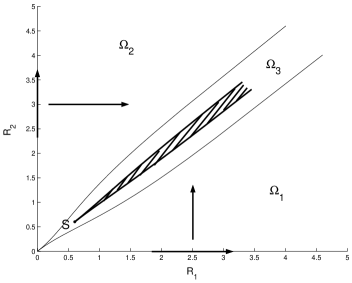
Figure 2: Distributed successive refinement for the quadratic Gaussian CEO problem

In Fig. 2, the arrows denote the possible directions for the distributed successive refinement in $\Omega_{1}$ and $\Omega_{3}$. For illustration, we pick a point $s$ in $\Omega_{2}$. The dark region is the set of points to which there exists a distributed successive refinement scheme from $s$. We can see that the distributed successive refinement behaves very differently in these three regions.

IV Conclusion

We discussed two closely related problems in distributed source coding: The first one is how to decompose a high complexity distributed source code into low complexity codes; The second one is how to construct a high rate distributed source code using low rate codes via distributed successive refinement. It turns out that, at least for the quadratic Gaussian CEO problem, the successive Wyner-Ziv coding scheme gives the answer to both problems. Besides the features (say, low complexity and robustness) we discussed in the paper, the concatenable chain structure of the successive Wyner-Ziv coding scheme seems especially attractive in wireless sensor networks, where channels are subject to fluctuation. In this case, by properly converting a high-rate distributed source code to a multistage code via the successive Wyner-Ziv coding scheme, one can match source rates to the channel rates adaptively.

[Proof of Lemma 3.5]

For any $r_{\mathcal{I}_{L}}\in\mathbb{R}^{L}_{+}$, define two set functions $f(\cdot,r_{\mathcal{I}_{L}}),f_{D}(\cdot,r_{\mathcal{I}_{L}}):2^{\mathcal{I}_{L}}\rightarrow\mathbb{R}_{+}$:

$$f(\mathcal{A},r_{\mathcal{I}_{L}}) = \frac{1}{2}\log\left(\frac{\frac{1}{\sigma^{2}_{X}}+\sum\limits_{i=1}^{L}\frac{1-\exp(-2r_{i})}{\sigma^{2}_{N_{i}}}}{\frac{1}{\sigma^{2}_{X}}+\sum\limits_{i\in\mathcal{I}_{L}\backslash\mathcal{A}}\frac{1-\exp(-2r_{i})}{\sigma^{2}_{N_{i}}}}\right)+\sum\limits_{i\in\mathcal{A}}r_{i},\forall\mbox{ nonempty set }\mathcal{A}\subseteq\mathcal{I}_{L},$$

$$f_{D}(\mathcal{A},r_{\mathcal{I}_{L}}) = \frac{1}{2}\log\frac{1}{D}-\frac{1}{2}\log\left(\frac{1}{\sigma^{2}_{X}}+\sum\limits_{i\in\mathcal{I}_{L}\backslash\mathcal{A}}\frac{1-\exp(-2r_{i})}{\sigma^{2}_{N_{i}}}\right)+\sum\limits_{i\in\mathcal{A}}r_{i},\forall\mbox{ nonempty set }\mathcal{A}\subseteq\mathcal{I}_{L},$$

and $f(\emptyset,r_{\mathcal{I}_{L}})=f_{D}(\emptyset,r_{\mathcal{I}_{L}})=0$.

Note that $f(\cdot,r_{\mathcal{I}_{L}})$ is a rank function and induces the contra-polymatroid $\mathcal{R}(r_{\mathcal{I}_{L}})$ defined in (17). Furthermore, for any nonempty set $\mathcal{A}\subseteq\mathcal{I}_{L}$,

$$f(\mathcal{A},r_{\mathcal{I}_{L}})-f_{D}(\mathcal{A},r_{\mathcal{I}_{L}}) = \frac{1}{2}\log\left(\frac{1}{\sigma^{2}_{X}}+\sum\limits_{i=1}^{L}\frac{1-\exp(-2r_{i})}{\sigma^{2}_{N_{i}}}\right)-\frac{1}{2}\log\frac{1}{D}.$$ (79)

By the supermodular property of $f(\cdot,r_{\mathcal{I}_{L}})$ and the equation (79), we can establish that, for any $r_{\mathcal{I}_{L}}$ satisfying $r_{i}>0$ $(\forall i\in\mathcal{I}_{L})$ and nonempty sets $\mathcal{S},\mathcal{T}\subseteq\mathcal{I}_{L}$,

• $$f(\mathcal{S},r_{\mathcal{I}_{L}})+f(\mathcal{T},r_{\mathcal{I}_{L}})<f(\mathcal{S}\cup\mathcal{T},r_{\mathcal{I}_{L}})+f(\mathcal{S}\cap\mathcal{T},r_{\mathcal{I}_{L}});$$ (80)

• If $1/\sigma^{2}_{X}+\sum_{i=1}^{L}(1-\exp(-2r_{i}))/\sigma^{2}_{N_{i}}\geq 1/D$, and $\mathcal{S}\nsubseteq\mathcal{T}$, $\mathcal{T}\nsubseteq\mathcal{S}$, then

  $$f_{D}(\mathcal{S},r_{\mathcal{I}_{L}})+f_{D}(\mathcal{T},r_{\mathcal{I}_{L}})<f_{D}(\mathcal{S}\cup\mathcal{T},r_{\mathcal{I}_{L}})+f_{D}(\mathcal{S}\cap\mathcal{T},r_{\mathcal{I}_{L}}).$$ (81)

It was shown in [34] that

$$\mathcal{R}(D)=\bigcup\limits_{r_{\mathcal{I}_{L}}\in\mathcal{F}(D)}\left\{R_{\mathcal{I}_{L}}:\sum\limits_{i\in\mathcal{A}}R_{i}\geq f_{D}(\mathcal{A},r_{\mathcal{I}_{L}}),\forall\mbox{ nonempty set }\mathcal{A}\subseteq\mathcal{I}_{L}\right\},$$ (82)

where $\mathcal{F}(D)$ is defined in (19). Hence there must exist a vector $r_{\mathcal{I}_{L}}\in\mathbb{R}^{L}_{+}$ satisfying the constraints (52) and (53) in Lemma III.5, i.e.,

$$\sum\limits_{i\in\mathcal{A}}R_{i}\geq f_{D^{*}(R_{\mathcal{I}_{L}})}(\mathcal{A},r_{\mathcal{I}_{L}}),\quad\forall\mbox{ nonempty set }\mathcal{A}\subseteq\mathcal{I}_{L},$$ (83)

and

$$\frac{1}{\sigma^{2}_{X}}+\sum\limits_{i=1}^{L}\frac{1-\exp(-r_{i})}{\sigma^{2}_{N_{i}}}\geq\frac{1}{D^{*}(R_{\mathcal{I}_{L}})}.$$ (84)

Let $\mathcal{G}=\{i\in\mathcal{I}_{L}:r_{i}>0\}$. Then (83) and (84) reduce to the following constraints:

$$\sum\limits_{i\in\mathcal{A}}R_{i}\geq f_{D^{*}(R_{\mathcal{I}_{L}})}(\mathcal{A},r_{\mathcal{I}_{L}}),\quad\forall\mbox{ nonempty set }\mathcal{A}\subseteq\mathcal{G},$$ (85)

and

$$\frac{1}{\sigma^{2}_{X}}+\sum\limits_{i\in\mathcal{G}}\frac{1-\exp(-r_{i})}{\sigma^{2}_{N_{i}}}\geq\frac{1}{D^{*}(R_{\mathcal{I}_{L}})}.$$ (86)

are still active. Thus without loss of generality, we can assume $\mathcal{G}=\mathcal{I}_{L}$.

It can be shown that in (83), if the constraints on $\sum_{i\in\mathcal{S}}R_{i}$ and $\sum_{i\in\mathcal{T}}R_{i}$ are tight, then either $\mathcal{S}\subseteq\mathcal{T}$ or $\mathcal{T}\subseteq\mathcal{S}$. Otherwise

$$f_{D^{*}(R_{\mathcal{I}_{L}})}(\mathcal{S},r_{\mathcal{I}_{L}})+f_{D^{*}(R_{\mathcal{I}_{L}})}(\mathcal{T},r_{\mathcal{I}_{L}})$$ (87)

$$= \sum\limits_{i\in\mathcal{S}}R_{i}+\sum\limits_{i\in\mathcal{T}}R_{i}$$ (88)

$$= \sum\limits_{i\in\mathcal{S}\cup\mathcal{T}}R_{i,j}+\sum\limits_{i\in\mathcal{S}\cap\mathcal{T}}R_{i}$$ (89)

$$\geq f_{D^{*}(R_{\mathcal{I}_{L}})}(\mathcal{S}\cup\mathcal{T},r_{\mathcal{I}_{L}})+f_{D^{*}(R_{\mathcal{I}_{L}})}(\mathcal{S}\cap\mathcal{T},r_{\mathcal{I}_{L}}),$$ (90)

contradictory to (81). Let $\mathcal{\widetilde{A}}=\bigcap_{k\in\mathcal{I}_{K}}\mathcal{A}_{k}$, where $\mathcal{A}_{k}(k\in\mathcal{I}_{K})$ are the sets for which the constraints on $\sum_{i\in\mathcal{A}_{k}}R_{i}$ are tight in (83). If there is no such an $\mathcal{A}_{k}$, let $\mathcal{\widetilde{A}}=\mathcal{I}_{L}$. $\mathcal{\widetilde{A}}$ is thus always nonempty.

Now suppose

$$\frac{1}{\sigma^{2}_{X}}+\sum\limits_{i=1}^{L}\frac{1-\exp(-r_{i})}{\sigma^{2}_{N_{i}}}>\frac{1}{D^{*}(R_{\mathcal{I}_{L}})}.$$ (91)

Pick any $i^{*}\in\widetilde{A}$, we can decreases $r_{i^{*}}$ to $r_{i^{*}}-\delta$ for some $\delta>0$ so that all the constraints in (83) and (91) become non-tight. Then we can decrease $D^{*}(R_{\mathcal{I}_{L}})$ to $D^{*}(R_{\mathcal{I}_{L}})-\epsilon$ for some $\epsilon>0$ without violating any constraints in (83) and (91). By (82) we have $R_{\mathcal{I}_{L}}\in\mathcal{R}(D^{*}(R_{\mathcal{I}_{L}})-\epsilon)$, contradictory to the definition of $D^{*}(R_{\mathcal{I}_{L}})$. Hence we can conclude that (54) holds, i.e.,

$$\frac{1}{\sigma^{2}_{X}}+\sum\limits_{i=1}^{L}\frac{1-\exp(-r_{i})}{\sigma^{2}_{N_{i}}}=\frac{1}{D^{*}(R_{\mathcal{I}_{L}})}.$$ (92)

Now we proceed to show that $r_{\mathcal{I}_{L}}$ must be unique.

It is easy to check that $1/\sigma^{2}_{X}+\sum_{i=1}^{L}(1-\exp(-2r_{i}))/\sigma^{2}_{N_{i}}$ is a strict concave function of $r_{\mathcal{I}_{L}}$ and for any nonempty set $\mathcal{A}\subseteq\mathcal{I}_{L}$, $f_{D}(\mathcal{A},r_{\mathcal{I}_{L}})$ is convex in $r_{\mathcal{I}_{L}}$.

Suppose both $r^{\prime}_{\mathcal{I}_{L}}$ and $r^{\prime\prime}_{\mathcal{I}_{L}}\in\mathbb{R}^{L}_{+}$ satisfy the constraints (83) and (84), and there exists some $i^{*}$ such that $r^{\prime}_{i^{*}}\neq r^{\prime\prime}_{i^{*}}$. We shall first show that $r^{\prime}_{i^{*}},r^{\prime\prime}_{i^{*}}$ are both finite. If not, without loss of generality suppose $r^{\prime}_{i^{*}}=\infty$, which implies that $R_{i^{*}}=\infty$. Now construct a new vector $r^{\prime\prime\prime}_{\mathcal{I}_{L}}$ such that $r^{\prime\prime\prime}_{i}=r^{\prime}_{i}=\infty$ if $i=i^{*}$ and $r^{\prime\prime\prime}_{i}=r^{\prime\prime}_{i}$ otherwise. Note: we have $r^{\prime\prime\prime}_{i^{*}}>r^{\prime\prime}_{i^{*}}$. It is easy to check that $r^{\prime\prime\prime}_{\mathcal{I}_{L}}$ satisfies the constraints (83) and (84) (Note: we let $\infty-\infty=0$). But we have

$$\frac{1}{\sigma^{2}_{X}}+\sum\limits_{i=1}^{L}\frac{1-\exp(-2r^{\prime\prime\prime}_{i})}{\sigma^{2}_{N_{i}}}>\frac{1}{\sigma^{2}_{X}}+\sum\limits_{i=1}^{L}\frac{1-\exp(-2r^{\prime\prime}_{i})}{\sigma^{2}_{N_{i}}}=\frac{1}{D^{*}(R_{\mathcal{I}_{L}})},$$ (93)

which is contradictory to (92).

Now let $\overline{r}_{i}=(r^{\prime}_{i}+r^{\prime\prime}_{i})/2$ for all $i\in\mathcal{I}_{L}$. Note that $\overline{r}_{i^{*}}$ is equal to neither $r^{\prime}_{i^{*}}$ nor $r^{\prime\prime}_{i^{*}}$ since $r^{\prime}_{i^{*}}\neq r^{\prime\prime}_{i^{*}}$ and both are finite. It is obvious that $\overline{r}_{\mathcal{I}_{L}}\in\mathbb{R}_{+}^{L}$. Furthermore, we have

$$\frac{1}{\sigma^{2}_{X}}+\sum\limits_{i=1}^{L}\frac{1-\exp(-\overline{r}_{i})}{\sigma^{2}_{N_{i}}} \geq \frac{1}{\sigma^{2}_{X}}+\frac{1}{2}\sum\limits_{i=1}^{L}\frac{1-\exp(-r^{\prime}_{i})}{\sigma^{2}_{N_{i}}}+\frac{1}{2}\sum\limits_{i=1}^{L}\frac{1-\exp(-r^{\prime\prime}_{i})}{\sigma^{2}_{N}}$$ (94)

$$\geq \frac{1}{D^{*}(R_{\mathcal{I}_{L}})},$$ (95)

and

$$\sum\limits_{i\in\mathcal{A}}R_{i} \geq \frac{1}{2}f_{D^{*}(R_{\mathcal{I}_{L}})}(\mathcal{A},r^{\prime}_{\mathcal{I}_{L}})+\frac{1}{2}f_{D^{*}(R_{\mathcal{I}_{L}})}(\mathcal{A},r^{\prime\prime}_{\mathcal{I}_{L}})$$ (96)

$$\geq f_{D^{*}(R_{\mathcal{I}_{L}})}(\mathcal{A},\overline{r}_{\mathcal{I}_{L}}),\quad\forall\mbox{ nonempty set }\mathcal{A}\subseteq\mathcal{I}_{L}.$$ (97)

Hence $\overline{r}_{\mathcal{I}_{L}}$ satisfies the constraints (83) and (84). Since $1/\sigma^{2}_{X}+\sum_{i=1}^{L}(1-\exp(-2r_{i}))/\sigma^{2}_{N_{i}}$ is a strictly concave function of $r_{\mathcal{I}_{L}}$, the inequality in (94) is strict, which results in a contradiction with (92).

Now only (55) remains to be proved. We shall first show that $r^{*}_{i}(R_{\mathcal{I}_{L}})=0$ implies $R_{i}=0$. Without loss of generality, suppose $r^{*}_{L}(R_{\mathcal{I}_{L}})=0$. Then it is easy to check that (83) still holds if we set $R_{L}=0$ on its left hand side. So if $R_{L}>0$, we can increase $r^{*}_{L}(R_{\mathcal{I}_{L}})$ by a small amount without violating (83) and (84), which is contradictory to the fact that $r^{*}_{L}(R_{\mathcal{I}_{L}})$ is unique. Hence without loss of generality, we can assume $r^{*}_{i}(R_{\mathcal{I}_{L}})>0$ for all $i\in\mathcal{I}_{L}$. Otherwise by restricting to the set $\mathcal{G}=\{i\in\mathcal{I}_{L}:r^{*}_{i}(R_{\mathcal{I}_{L}})>0\}$, the following argument can still be applied.

Since (54) holds, the righthand side of (83) becomes $f(\mathcal{A},r^{*}_{\mathcal{I}_{L}}(R_{\mathcal{I}_{L}}))$. By (80), it can be shown that if in (83), the constraints on $\sum_{i\in\mathcal{S}}R_{i}$ and $\sum_{i\in\mathcal{T}}R_{i}$ are tight, then either $\mathcal{S}\subseteq\mathcal{T}$ or $\mathcal{T}\subseteq\mathcal{S}$. Let $\mathcal{\widetilde{A}}=\bigcup_{k\in\mathcal{I}_{K}}\mathcal{A}_{k}$, where $\mathcal{A}_{k}(k\in\mathcal{I}_{K})$ are the sets for which the constraints on $\sum_{i\in\mathcal{A}_{k}}R_{i}$ are tight in (83). If there is no such an $\mathcal{A}_{k}$, let $\mathcal{\widetilde{A}}=\emptyset$.

If $\mathcal{\widetilde{A}}=\mathcal{I}_{L}$, we are done. Otherwise pick any $i^{*}\in\mathcal{I}_{L}\backslash\mathcal{\widetilde{A}}$. We can increase $r^{*}_{i^{*}}(R_{\mathcal{I}_{L}})$ to $r^{*}_{i^{*}}(R_{\mathcal{I}_{L}})+\delta$ for some $\delta>0$ without violating any constraints in (52) and (53), which is contradictory to the uniqueness of $r^{*}_{i^{*}}(R_{\mathcal{I}_{L}})$.

References

• [1] D. Schongberg, K. Ramchandran and S. S. Pradhan, โ€œDistributed code constructions for the entire Slepian-Wolf rate region for arbitrarily correlated sources,โ€ Proc. DCC04, Snowbird, UT, Mar. 2004.
• [2] T. P. Coleman, A. H. Lee, M. Mรฉdard and M. Effos, โ€œOn some new approaches to practical Slepian-Wolf compression inspired by channel coding,โ€ Proc. DCC04, Snowbird, UT, Mar. 2004.
• [3] S. Cheng and Z. Xiong, โ€œSuccessive refinement for the Wyner-Ziv problem and layered code design,โ€ Proc. DCC04, Snowbird, UT, Mar. 2004.
• [4] D. Slepian and J. K. Wolf, โ€œNoiseless coding of correlated information sources,โ€ IEEE Trans. Info. Theory, vol.IT-19, pp. 471-480, Jul. 1973.
• [5] A. D. Wyner and J. Ziv, โ€œThe rate-distortion function for source coding with side information at the decoder,โ€ IEEE Trans. Info. Theory, vol. 22, no. 1, pp. 1-10, Jan. 1976.
• [6] J. Edmonds, โ€œSubmodular functions, matroids and certain polyhedra, in Combinatorial structures and their applications (R. Guy, H. Hanani, N. Sauer, and J. Schonheim, eds.), pp. 69-87, Gordon and Breach, New York, 1970. (Proc. Calgary Int. Conf. 1969).
• [7] D. N. C. Tse and S. V. Hanly, โ€œMultiaccess fading channels-part I: polymatroid structure, optimal resource allocation and throughput capacities,โ€ IEEE Trans. Info. Theory, vol. 44, pp. 2796-2815, Nov. 1998.
• [8] B. Rimoldi and R. Urbanke, โ€œAsynchronous Slepian-Wolf coding via source-splitting,โ€ in IEEE International Symposium on Information Theory, Ulm, Germany, June 29 - July 4 1997, p. 271.
• [9] R. Zamir, S. Shamai and U. Erez, โ€œNested linear/lattice codes for structured multiterminal binning,โ€ IEEE Trans. Info. Theory, vol. 48, pp. 1250-1276, June 2002.
• [10] A. B. Carleial, โ€œOn the capacity of multiple-terminal communication networks,โ€ Ph.D. dissertation, Stanford Univ., Stanford, CA, Aug. 1975.
• [11] B. Rimoldi and R. Urbanke, โ€œA rate-splitting approach to the Gaussian multiple- access channel,โ€ IEEE Trans. Inform. Theory, vol. 42, pp. 364-375, Mar. 1996.
• [12] A. J. Grant, B. Rimoldi, R. L. Urbanke, and P. A. Whiting, โ€œRate-splitting multiple access for discrete memoryless channels,โ€ IEEE Trans. Inform. Theory, vol. 47, no. 3, pp. 873-890, Mar. 2001.
• [13] B. Rimoldi, โ€œGeneralized time sharing: a low-complexity capacity-achieving multiple- access technique,โ€ IEEE Trans. Inform. Theory, vol. 47, no. 6, pp. 2432-2442, Sept. 2001.
• [14] S. I. Gelโ€™fand and M. S. Pinsker, โ€œCoding of sources on the basis of observations with incomplete informationโ€. Problems of Information Transmission, 15(2):115-125, 1979.
• [15] T. J. Flynn and R. M. Gray, โ€œEncoding of correlated observations,โ€ IEEE Trans. Inform. Theory, vol.ย 33, pp.ย 773-787, Nov. 1987.
• [16] T. Berger, Z. Zhang, and H. Viswanathan, โ€œThe CEO problem,โ€ IEEE Trans. Inform. Theory, vol. 42, pp. 887-902, May 1996.
• [17] T. Berger, โ€œMultiterminal source coding,โ€ in The Information Theory Approach to Communications (G. Longo, ed.), vol. 229 of CISM Courses and Lectures, pp. 171-231, Springer-Verlag, Vienna/New York, 1978.
• [18] S. Y. Tung, โ€œMultiterminal source coding,โ€ Ph.D. dissertation, School of Electrical Engineering, Cornell Univ., Ithaca, NY, May 1978.
• [19] T. Berger, K. Housewright, J. Omura, S. Y. Tung, and J. Wolfowitz, โ€œAn upper bound on the rate-distortion function for source coding with partial side information at the decoder,โ€ IEEE Trans. Inform. Theory, vol. IT-25, pp.664-666, Nov., 1979.
• [20] J. Kรถrner and K. Marton, โ€œHow to encode the modulo-two sum of binary sources (Corresp.),โ€ IEEE Trans. on Inform. Theory, vol. 25, pp. 219-221, Mar 1979.
• [21] P. Viswanath, โ€œSum rate of multiterminal gaussian source coding,โ€ in Network Information Theory (P. Gupta, G. Kramer, and A. Wijngaarden, eds.), DIMACS: Series in Discrete Mathematics and Theoretical Computer Science, American Mathematical Society and DIMACS.
• [22] J. Chen, X. Zhang, T. Berger and S. B. Wicker, โ€œAn upper bound on the sum- Rate distortion function and its corresponding rate allocation schemes for the CEO problem,โ€ IEEE J. Select. Areas Commun., vol.ย 22, pp.ย 977-987, Aug. 2004.
• [23] H. G. Eggleston, Convexity. Cambridge, England: Cambridge Univ. Press, 1958.
• [24] T. M. Cover and J. A. Thomas, Elements of Information Theory. New York: Wiley, 1991.
• [25] S. C. Draper and G. W. Wornell, โ€œSide information aware coding strategies for sensor networks,โ€ IEEE J. Select. Areas Commun., vol.ย 22, pp.ย 966-976, Aug. 2004.
• [26] B. Rimoldi and R. Urbanke, โ€œOn the structure of the dominant face of multiple access channels,โ€ Proc. Information Theory and Communications Workshop, June 20-25, 1999, Kruger National Park, South Africa, pp.ย 12-14.
• [27] R. Ahlswede, โ€œMulti-way communication channels,โ€ in Proc. 2nd Int. Symp. Information Theory. Budapest, Hungary: Hungarian Acad. Sci., 1973, pp. 23-52.
• [28] H. Liao, โ€œMultiple access channels,โ€ Ph.D. dissertation, Dept. Elec. Eng., Univ. Hawaii, Honolulu, 1972.
• [29] A. D. Wyner, โ€œThe rate-distortion function for source coding with side information at the decoder-II: General sources,โ€ Inform. Contr., vol.ย 38, pp.ย 60-80, Jul. 1978.
• [30] Y. Oohama, โ€œGaussian multiterminal source coding,โ€ IEEE Trans. on Inform. Theory, vol.ย 43, no.ย 6, pp.ย 1912-1923, Nov. 1997.
• [31] Y. Oohama, โ€œThe rate-distortion function for the quadratic Gaussian CEO problem,โ€ IEEE Trans. on Inform. Theory, vol. 44, no. 3, pp. 1057-1070, May 1998.
• [32] H. Viswanathan and T. Berger, โ€œThe quadratic Gaussian CEO problem,โ€ IEEE Trans. Inform. Theory, vol. 43, pp. 1549-1559, Sept. 1997.
• [33] Y. Oohama, โ€œRate-distortion theory for Gaussian multiterminal source coding systems with several side informations at the decoder,โ€ IEEE Trans. on Inform Theory, vol. 51, pp. 2577-2593, July 2005.
• [34] V. Prabhakaran, D. Tse and K. Ramchandran, โ€œRate region of the quadratic Gaussian CEO problem,โ€ Proc. International Symposium on Information Theory, June 27-July 2, 2004, Chicago, USA, pp.ย 119.
• [35] S. Boyd and L. Vandenberghe, Convex Optimization. Cambridge, U.K.: Cambridge Univ. Press, 2004.
• [36] V. Koshelev, โ€œHierarchical coding of discrete sources,โ€ Probl. Pered. Inform., vol.ย 16, no.ย 3, pp.ย 31-49, 1980.
• [37] V. Koshelev, โ€œEstimation of mean error for a discrete successive-approximation scheme,โ€ Probl. Pered. Inform., vol.ย 17, no.ย 3, pp.ย 20-33, 1981.
• [38] W. H. R. Equitz and T. M. Cover, โ€œSuccessive refinement of information,โ€ IEEE Trans. on Inform. Theory, vol. 37, pp. 269-274, Mar. 1991.
• [39] B. Rimoldi, โ€œSuccessive refinement of information: Characterization of the achievable rates,โ€ IEEE Trans. Inform. Theory, vol.ย 40, pp.ย 253-259, Jan. 1994.
• [40] Y. Steinberg and N. Merhav, โ€œOn successive refinement for the Wyner-Ziv problem,โ€ IEEE Trans. Inform. Theory, vol.ย 50, pp.ย 1636- 1654, Aug. 2004.