Unbiased Matrix Rounding

Abstract

We show several ways to round a real matrix to an integer one such that the rounding errors in all rows and columns as well as the whole matrix are less than one. This is a classical problem with applications in many fields, in particular, statistics.

We improve earlier solutions of different authors in two ways. For rounding matrices of size $m\times n$, we reduce the runtime from $O((mn)^{2})$ to $O(mn\log(mn))$. Second, our roundings also have a rounding error of less than one in all initial intervals of rows and columns. Consequently, arbitrary intervals have an error of at most two. This is particularly useful in the statistics application of controlled rounding.

The same result can be obtained via (dependent) randomized rounding. This has the additional advantage that the rounding is unbiased, that is, for all entries $y_{ij}$ of our rounding, we have $E(y_{ij})=x_{ij}$, where $x_{ij}$ is the corresponding entry of the input matrix.

1 Introduction

In this paper, we analyze a rounding problem with strong connections to statistics, but also to different areas in discrete mathematics, computer science, and operations research. We show how to round a matrix to an integer one such that rounding errors in intervals of rows and columns are small.

Let $m,n$ be positive integers. For some set $S$, we write $S^{m\times n}$ to denote the set of $m\times n$ matrices with entries in $S$. For real numbers $a,b$ let $[a..b]:=\{z\in{\mathbb{Z}}\mid a\leq z\leq b\}$. We show the following.

Theorem 1.

For all $X\in[0,1)^{m\times n}$ a rounding $Y\in\{0,1\}^{m\times n}$ such that

$$\forall b\in[1..n],\;i\in[1..m] : \bigg{|}\sum_{j=1}^{b}(x_{ij}-y_{ij})\bigg{|}<1,$$

$$\forall b\in[1..m],\;j\in[1..n] : \bigg{|}\sum_{i=1}^{b}(x_{ij}-y_{ij})\bigg{|}<1,$$

$$\bigg{|}\sum_{i=1}^{m}\sum_{j=1}^{n}(x_{ij}-y_{ij})\bigg{|}<1$$

can be computed in time $O(mn\log(mn))$.

This result extends the famous rounding lemma of Baranyai [3] and several results on controlled rounding in statistics by Bacharach [2] and Causey, Cox and Ernst [7].

1.1 Baranyai’s Rounding Lemma and Applications in Statistics

Baranyai [3] used a weaker version of Theorem 1 to obtain his well-known results on coloring and partitioning complete uniform hypergraphs. He showed that any matrix can be rounded such that the errors in all rows, all columns and the whole matrix are less than one. He used a formulation as flow problem to prove this statement. This yields an inferior runtime than the bound in Theorem 1. However, algorithmic issues were not his focus.

In statistics, Baranyai’s result was independently obtained by Bacharach [2] (in a slightly weaker form) and again independently by Causey, Cox and Ernst [7]. There are two statistical applications for such rounding results. Note first that instead of rounding to integers, our result also applies to rounding to multiples of any other base (e.g., multiples of 10). Such a rounding can be used to improve the readability of data tables.

The main reason, however, to apply such a rounding procedure is confidentiality protection. Frequency counts that directly or indirectly disclose small counts may permit the identification of individual respondents. There are various methods to prevent this [25], one of which is controlled rounding [9]. Here, one tries to round an $(m+1)\times(n+1)$-table $\tilde{X}$ given by

$$\begin{array}[]{c|c}\left(x_{ij}\right)_{\genfrac{}{}{0.0pt}{}{i=1\ldots m}{j=1\ldots n}}&\left(\sum_{j=1}^{n}x_{ij}\right)_{i=1\ldots m}\\ \\ \hline\cr\\ \left(\sum_{i=1}^{m}x_{ij}\right)_{j=1\ldots n}&\sum_{i=1}^{m}\sum_{j=1}^{n}x_{ij}\\ \end{array}\noindent$$

to an $(m+1)\times(n+1)$-table $\tilde{Y}$ such that additivity is preserved, i.e., the last row and column of $\tilde{Y}$ contain the associated totals of $\tilde{Y}$. In our setting we round the $m\times n$-matrix $X$ defined by the $mn$ inner cells of the table $\tilde{X}$ to obtain a controlled rounding.

The additivity in the rounded table allows to derive information on the row and column totals of the original table. In contrast to other rounding algorithms, our result also permits to retrieve further reliable information from the rounded matrix, namely on the sums of consecutive elements in rows or columns. Such queries may occur if there is a linear ordering on statistical attributes. Here an example. Let $x_{ij}$ be the number of people in country $i$ that are $j$ years old. Say $Y$ is such that $\frac{1}{1000}Y$ is a rounding of $\frac{1}{1000}X$ as in Theorem 1. Now $\sum_{j=20}^{40}y_{ij}$ is the number of people in country $i$ that are between $20$ and $40$ years old, apart from an error of less than $2000$. Note that such guarantees are not provided by the results of Baranyai [3], Bacharach [2], and Causey, Cox and Ernst [7].

1.2 Unbiased Rounding

In Section 4, we present a randomized algorithm computing roundings as in Theorem 1. It has the additional property that each matrix entry is rounded up with probability equal to its fractional value. This is known as randomized rounding [20] in computer science and as unbiased controlled rounding [8, 15] in statistics. Here, a controlled rounding is computed such that the expected values of each table entry (including the totals) equals its fractional value in the original table.

To state our result more precisely, we introduce the following notation. For $x\in{\mathbb{R}}$ write $\lfloor x\rfloor:=\max\{z\in{\mathbb{Z}}\mid z\leq r\},\lceil x\rceil:=\min\{z\in{\mathbb{Z}}\mid z\geq r\}$ and $\{x\}:=x-\lfloor x\rfloor$.

Definition 2.

Let $x\in{\mathbb{R}}$. A random variable $y$ is called randomized rounding of $x$, denoted $y\approx x$, if $\Pr(y=\lfloor x\rfloor+1)=\{x\}$ and $\Pr(y=\lfloor x\rfloor)=1-\{x\}$. For a matrix $X\in{\mathbb{R}}^{m\times n}$, we call an ${m\times n}$ matrix-valued random variable $Y$ randomized rounding of $X$ if $y_{ij}\approx x_{ij}$ for all $i\in[1..m],j\in[1..n]$.

We then get the following randomized version of Theorem 1.

Theorem 3.

Let $X\in[0,1)^{m\times n}$ be a matrix having entries of binary length at most $\ell$. Then a randomized rounding $Y$ fulfilling the additional constraints that

$$\forall b\in[1..n],\;i\in[1..m] : \sum_{j=1}^{b}x_{ij}\approx\sum_{j=1}^{b}y_{ij},$$

$$\forall b\in[1..m],\;j\in[1..n] : \sum_{i=1}^{b}x_{ij}\approx\sum_{i=1}^{b}y_{ij},$$

$$\sum_{i=1}^{m}\sum_{j=1}^{n}x_{ij}\approx\sum_{i=1}^{m}\sum_{j=1}^{n}y_{ij}$$

can be computed in time $O(mn\ell)$.

For a matrix with arbitrary entries $x_{ij}:=\sum_{d=1}^{\ell}x_{ij}^{(d)}2^{-d}+x_{ij}^{\prime}$ where $x_{ij}^{\prime}<2^{-\ell}$ and $x_{ij}^{(d)}\in\{0,1\}$ for $i\in[1..m],j\in[1..n],d\in[1..\ell]$, we may use the $\ell$ highest bits to get an approximate randomized rounding. If (before doing so) we round the remaining part $x_{ij}^{\prime}$ of each entry to $2^{-\ell}$ with probability $2^{\ell}x_{ij}^{\prime}$ and to $0$ otherwise, we still have that $Y\approx X$, but we introduce an additional error of at most $2^{-\ell}mn$ in the constraints of Theorem 3.

1.3 Other Applications

One of the most basic rounding results states that any sequence $x_{1},\ldots,x_{n}$ of numbers can be rounded to an integer one $y_{1},\ldots,y_{n}$ such that the rounding errors $|\sum_{j=a}^{b}(x_{j}-y_{j})|$ are less than one for all $a,b\in[1..n]$. Such roundings can be computed efficiently in linear time by a one-pass algorithm resembling Kadane’s scanning algorithm (described in Bentley’s Programming Pearls [5]). Extensions in different directions have been obtained in [11, 12, 17, 21, 23]. This rounding problem has found a number of applications, among others in image processing [1, 22].

Theorem 1 extends this result to two-dimensional sequences. Here the rounding error in arbitrary intervals of a row or column is less than two. In [14] a lower bound of 1.5 is shown for this problem. Thus an error of less than one as in the one-dimensional case cannot be achieved.

Rounding a matrix while considering the errors in column sums and partial row sums also arises in scheduling [6, 18, 19, 24]. For this, however, one does not need our result in full generality. It suffices to use the linear-time one-pass algorithm given in [14]. This algorithm rounds a matrix having unit column sums and can be extend to compute a quasi rounding for arbitrary matrices. While this algorithm keeps the error in all initial row intervals small, for columns only the error over the whole column is considered.

1.4 Knuth’s Two-way Rounding

In [17], Knuth showed how to round a sequence of $n$ real numbers $x_{i}$ to $y_{i}\in\left\{\lfloor x_{i}\rfloor,\lceil x_{i}\rceil\right\}$ such that for two given permutations $\sigma_{1},\sigma_{2}\in S_{n}$, we have both $|\sum_{i=1}^{k}(x_{\sigma_{1}(i)}-y_{\sigma_{1}(i)})|\leq n/(n+1)$ and $|\sum_{i=1}^{k}(x_{\sigma_{2}(i)}-y_{\sigma_{2}(i)})|\leq n/(n+1)$ for all $k$. Knuth’s proof uses integer flows in a certain network [16]. On account of this his worst-case runtime is quadratic.

One application Knuth mentioned in [17] is that of matrix rounding. For this, simply choose a permutation $\sigma_{1}$ that enumerates the $x_{ij}$ row by row, and a permutation $\sigma_{2}$ that enumerates the $x_{ij}$ column by column. Applying Knuth’s algorithm to these permutations gives a rounding with errors smaller than one in all initial row and column intervals.

2 Preliminaries

In this section, we provide two easy extensions of the result stated in the introduction. First, we immediately obtain rounding errors of less than two in arbitrary intervals in rows and columns. This is supplied by the following lemma.

Lemma 4.

Let $Y$ be a rounding of a matrix $X$ such that the errors $|\sum_{j=1}^{b}(x_{ij}-y_{ij})|$ in all initial intervals of rows are at most $d$. Then the errors in arbitrary intervals of rows are at most $2d$, that is, for all $i\in[1..m]$ and all $1\leq a\leq b\leq n$,

$$\bigg{|}\sum_{j=a}^{b}(x_{ij}-y_{ij})\bigg{|}\leq 2d.$$

This also holds for column intervals, i.e., if the errors $|\sum_{i=1}^{b}(x_{ij}-y_{ij})|$ in all initial intervals of columns are at most $d^{\prime}$, then the errors $|\sum_{i=a}^{b}(x_{ij}-y_{ij})|$ in arbitrary intervals of columns are at most $2d^{\prime}$.

Proof.

Let $i\in[1..m]$ and $1\leq a\leq b\leq n$. Then

$$\bigg{|}\sum_{j=a}^{b}(x_{ij}-y_{ij})\bigg{|} = \bigg{|}\sum_{j=1}^{b}(x_{ij}-y_{ij})-\sum_{j=1}^{a-1}(x_{ij}-y_{ij})\bigg{|}$$

$$\leq \bigg{|}\sum_{j=1}^{b}(x_{ij}-y_{ij})\bigg{|}+\bigg{|}\sum_{j=1}^{a-1}(x_{ij}-y_{ij})\bigg{|}\ \leq\ 2d.$$

∎

From now on, we will only consider matrices having integral row and column sums. This is justified by the following lemma.

Lemma 5.

Assume that for any $X\in{\mathbb{R}}^{m\times n}$ with integral column and row sums a rounding $Y\in{\mathbb{Z}}^{m\times n}$ such that

$$\forall b\in[1..n],\;i\in[1..m] : \bigg{|}\sum_{j=1}^{b}(x_{ij}-y_{ij})\bigg{|}<1,$$ (1)

$$\forall b\in[1..m],\;j\in[1..n] : \bigg{|}\sum_{i=1}^{b}(x_{ij}-y_{ij})\bigg{|}<1$$ (2)

can be computed in time T(m,n). Then for all $\tilde{X}\in{\mathbb{R}}^{m\times n}$ with arbitrary column and row sums a rounding $\tilde{Y}\in{\mathbb{Z}}^{m\times n}$ satisfying (1), (2) and

$$\bigg{|}\sum_{i=1}^{m}\sum_{j=1}^{n}(x_{ij}-y_{ij})\bigg{|}<1$$ (3)

can be computed in time $T(m+1,n+1)+O(mn)$.

Proof.

Given an arbitrary matrix $\tilde{X}\in{\mathbb{R}}^{m\times n}$, we add an extra row taking what is missing towards integral column sums and add an extra column taking what is missing towards integral row sums. Hence, let $X\in{\mathbb{R}}^{(m+1)\times(n+1)}$ be such that

$$x_{ij}=\tilde{x}_{ij} \text{ for all }i\in[1..m],\;j\in[1..n],$$

$$x_{m+1,j}=\bigg{\lceil}\sum_{i=1}^{m}\tilde{x}_{ij}\bigg{\rceil}-\sum_{i=1}^{m}\tilde{x}_{ij} \text{ for all }j\in[1..n],$$

$$x_{i,n+1}=\bigg{\lceil}\sum_{j=1}^{n}\tilde{x}_{ij}\bigg{\rceil}-\sum_{j=1}^{n}\tilde{x}_{ij} \text{ for all }i\in[1..m],$$

$$x_{m+1,n+1}=\bigg{\lceil}\sum_{i=1}^{m}\tilde{x}_{i,n+1}\bigg{\rceil}-\sum_{i=1}^{m}\tilde{x}_{i,n+1} = \bigg{\lceil}\sum_{j=1}^{n}\tilde{x}_{m+1,j}\bigg{\rceil}-\sum_{j=1}^{n}\tilde{x}_{m+1,j}.$$

Clearly, $X$ has integral row and column sums. Therefore it can be rounded to $Y\in{\mathbb{Z}}^{(m+1)\times(n+1)}$ satisfying (1) and (2) in time $T(m+1,n+1)$.

For (3), observe that if a row (resp. column) sum is integral, the rounding error in the row (resp. column) is $0$. Then the rounding error in the whole matrix is also $0$, if all row and column sums are integral. Using this and the triangle inequality, we get inequality (3) as follows.

$$\bigg{|}\sum_{i=1}^{m}\sum_{j=1}^{n}(x_{ij}-y_{ij})\bigg{|} = \bigg{|}\sum_{i=1}^{m+1}\sum_{j=1}^{n+1}(x_{ij}-y_{ij})-\sum_{i=1}^{m+1}(x_{i,n+1}-y_{i,n+1})$$

$$-\sum_{j=1}^{n+1}(x_{m+1,j}-y_{m+1,j})+(x_{m+1,n+1}-y_{m+1,n+1})\bigg{|}$$

$$\leq 0+0+0+|x_{m+1,n+1}-y_{m+1,n+1}|<1.$$

By setting $\tilde{y}_{ij}=y_{ij}$ for all $i\in[1..m]$ and $j\in[1..n]$, we obtain the desired rounding $\tilde{Y}\in{\mathbb{Z}}^{m\times n}$. ∎

3 Bitwise Rounding

In this section, we present an alternative approach which will lead to a superior runtime. It uses a classical result on rounding problems, namely, that the problem of rounding arbitrary numbers can be reduced to the one of rounding half-integral numbers. For $X\in\{0,\tfrac{1}{2}\}^{m\times n}$, our rounding problem turns out to be much simpler. In fact, it can be solved in linear time.

3.1 The Binary Rounding Method

The following rounding method was introduced by Beck and Spencer [4] in 1984. They used it to prove the existence of two-colorings of ${\mathbb{N}}$ having small discrepancy in all arithmetic progressions of arbitrary length and bounded difference.

Given arbitrary numbers that have to be rounded, they use their binary expansion and (assuming all of them to be finite) round ‘digit by digit’. To do the latter, they only need to understand the corresponding rounding problem for half-integral numbers. That is, an $\ell$-bit number $x=x^{\prime}+\tfrac{1}{2}x^{\prime\prime},x^{\prime}\in\{0,\tfrac{1}{2}\}$ can be recursively rounded by rounding the $(\ell-1)$-bit number $x^{\prime\prime}$ to $y^{\prime\prime}\in\{0,1\}$ and then rounding $x^{\prime}+\tfrac{1}{2}y^{\prime\prime}\in\{0,\tfrac{1}{2},1\}$ to $y\in\{0,1\}$. The resulting rounding errors are at most twice the ones incurred by the half-integral roundings.

If some numbers do not have a finite binary expansion, one can use a sufficiently large finite length approximation. To get rid of additional errors caused by this, we invoke a slight refinement of the binary rounding method. In [10] it was proven that the extra factor of two can be reduced to an extra factor of $2(1-\frac{1}{2r})$, where $r$ is the number of rounding errors we want to keep small.

In our setting, the number of rounding errors is the number of all initial row and column intervals, i.e., $r=2mn$. In summary, we have the following.

Lemma 6.

Assume that for any $X\in\{0,\frac{1}{2}\}^{m\times n}$ a rounding $Y\in\{0,1\}^{m\times n}$ can be computed in time $T$ that satisfies

$$\forall b\in[1..n],\;i\in[1..m]:\bigg{|}\sum_{j=1}^{b}(x_{ij}-y_{ij})\bigg{|}\leq D,$$

$$\forall b\in[1..m],\;j\in[1..n]:\bigg{|}\sum_{i=1}^{b}(x_{ij}-y_{ij})\bigg{|}\leq D.$$

Then for all $\ell\in{\mathbb{N}}$ and $X\in[0,1)^{m\times n}$ a rounding $Y\in\{0,1\}^{m\times n}$ such that

$$\forall b\in[1..n],\;i\in[1..m]:\bigg{|}\sum_{j=1}^{b}(x_{ij}-y_{ij})\bigg{|}\leq 2(1-\tfrac{1}{4mn})D+2^{-\ell}b,$$

$$\forall b\in[1..m],\;j\in[1..n]:\bigg{|}\sum_{i=1}^{b}(x_{ij}-y_{ij})\bigg{|}\leq 2(1-\tfrac{1}{4mn})D+2^{-\ell}b$$

can be computed in time $O(\ell\,T)$.

3.2 Rounding Half-Integral Matrices

It remains to show how to solve the rounding problem for half-integral matrices. Based on Lemma 5, we can assume integrality of row and column sums.

Here is an outline of our approach. For each row and column, we consider the sequence of its $\tfrac{1}{2}$–entries and partition them into disjoint pairs of neighbors. From the two $\tfrac{1}{2}$s forming such a pair, exactly one is rounded to $1$ and the other to $0$. Thus, if such a pair is contained in an initial interval, it does not contribute to the rounding error.

To make the idea precise, assume some row contains exactly $2K$ entries of value $\tfrac{1}{2}$. We call the $(2k-1)$–th and $(2k)$–th $\tfrac{1}{2}$–entry of this row a row pair, for all $1\leq k\leq K$. The $\tfrac{1}{2}$s of a row pair are mutually referred to as row neighbors. Similarly, we define column pairs and column neighbors. Figure 1LABEL:sub@subfig:matrix shows a half-integral matrix together with row and column pairs marked by boxes. Since each $\tfrac{1}{2}$ belongs to a row pair and a column pair, the task of rounding is non-trivial.

Our solution makes use of an auxiliary graph ${\cal G}_{X}$ which contains the necessary information about row and column neighbors. Each $\tfrac{1}{2}$–entry is represented by a vertex that is labeled with the corresponding matrix indices. Each pair is represented by an edge connecting the vertices that correspond to the paired $\tfrac{1}{2}$s. Figure 1LABEL:sub@subfig:graph shows the auxiliary graph that belongs to the matrix of Figure 1LABEL:sub@subfig:matrix.

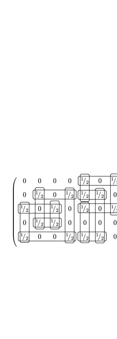
(a)

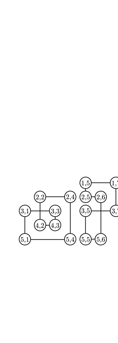
(b)

Figure 1: Example for the construction of an auxiliary graph. LABEL:sub@subfig:matrix Input matrix $X$ with its row and column pairs. LABEL:sub@subfig:graph Auxiliary graph ${\cal G}_{X}$. Vertices are labeled with matrix indices and edges connect vertices of row and column pairs. ${\cal G}_{X}$ is a disjoint union of even cycles.

We collect some properties of this auxiliary graph.

Lemma 7.

Let $X\in\{0,\tfrac{1}{2}\}^{m\times n}$ be a matrix with integral row and column sums.

1. Every vertex of ${\cal G}_{X}$ has degree 2.

2. ${\cal G}_{X}$ is a disjoint union of even cycles.

3. ${\cal G}_{X}$ is bipartite.

Proof.

(a) Because of the integrality of the row and column sums, the number of $\tfrac{1}{2}$–entries in each row and column is even. Hence each $\tfrac{1}{2}$–entry has a row and a column neighbor. In consequence, each vertex is incident with exactly two edges. (b) The edge sequence of a path in ${\cal G}_{X}$ corresponds to an alternating sequence of row and column pairs. Therefore any cycle in ${\cal G}_{X}$ consists of an even number of edges. Since each vertex has degree two, ${\cal G}_{X}$ is a disjoint union of cycles. (c) Clearly, every even cycle is bipartite. ∎

With this result, we are able to find the desired roundings.

Lemma 8.

Let $X\in\{0,\tfrac{1}{2}\}^{m\times n}$ and let $V_{0}\dot{\cup}V_{1}$ be a bipartition of ${\cal G}_{X}$. Define $Y=(y_{ij})\in\{0,1\}^{m\times n}$ by

$$y_{ij}=\begin{cases}0,&\text{if }x_{ij}=0\\ 0,&\text{if }x_{ij}=\tfrac{1}{2}\text{ and }(i,j)\in V_{0}\\ 1,&\text{if }x_{ij}=\tfrac{1}{2}\text{ and }(i,j)\in V_{1}.\end{cases}$$

Then $Y$ has the property that

$$\forall b\in[1..n],\;i\in[1..m] : \bigg{|}\sum_{j=1}^{b}(x_{ij}-y_{ij})\bigg{|}\leq\tfrac{1}{2},$$ (4)

$$\forall b\in[1..m],\;j\in[1..n] : \bigg{|}\sum_{i=1}^{b}(x_{ij}-y_{ij})\bigg{|}\leq\tfrac{1}{2}.$$ (5)

Proof.

Because $0$s of $X$ are maintained in $Y$, it suffices to consider $\tfrac{1}{2}$–entries to determine the rounding error in initial intervals. Since the rounded values for the $(2k-1)$-th and $(2k)$-th $\tfrac{1}{2}$–entry sum up to 1 by construction, there is no error in initial intervals that contain an even number of $\tfrac{1}{2}$s, and an error of $\tfrac{1}{2}$ if they contain an odd number of $\tfrac{1}{2}$s. ∎

After these considerations, we are able to present an algorithm that solves the problem in two steps: first we compute the auxiliary graph and afterwards the output matrix. To construct ${\cal G}_{X}$, we transform the input matrix $X$ column by column from left to right. Of course, generating the labeled vertices is trivial. The column neighbors are detected just by numbering the $\tfrac{1}{2}$–entries within a column from top to bottom. When there are $2k$ such entries, we insert an edge between the vertices with number $2i-1$ and $2i$ with $1\leq i\leq k$. The strategy to detect row neighbors is the same but we need more information. Therefore we store for each row the parity of its $\tfrac{1}{2}$–entries so far and, if the parity is odd, further a pointer to the last occurrence of $\tfrac{1}{2}$ in this row. Then, if the current $\tfrac{1}{2}$ is an even occurrence, we have a pointer to the preceding $\tfrac{1}{2}$, and are able to insert an edge between the corresponding vertices in ${\cal G}_{X}$.

The output matrix $Y$ can be computed from $X$ as follows. Every $0$ in $X$ is kept and every $\tfrac{1}{2}$–sequence that corresponds to a cycle in ${\cal G}_{X}$ is substituted by an alternating $0$–$1$–sequence. By Lemma 7, this is always possible. It does not matter which of the two alternating $0$–$1$ sequences we choose.

The graph ${\cal G}_{X}$ can be realized with adjacency lists (the vertex degree is always 2). The additional information per row can be realized by a simple pointer–array of length $m$ (a special nil–value indicates even parity).

Since the runtime of each step is bounded by the size of the input matrix, the entire algorithm takes time $O(mn)$. In addition to the constant amount of space we need for each of the $m$ rows, we store all $k$ entries of value $\tfrac{1}{2}$ in the auxiliary graph. This leads to a total space consumption of $O(m+k)$. Summarizing the above, we obtain the following lemma.

Lemma 9.

Let $X\in\{0,\tfrac{1}{2}\}^{m\times n}$. Then a rounding $Y\in\{0,1\}^{m\times n}$ satisfying the inequalities (4) and (5) can be computed in time $O(mn)$.

3.3 Final Result

By combining Lemma 6 and 9, we obtain the following result.

Theorem 10.

For all $\ell\in{\mathbb{N}}$ and $X\in[0,1)^{m\times n}$ a rounding $Y\in\{0,1\}^{m\times n}$ such that

$$\forall b\in[1..n],\;i\in[1..m]:\bigg{|}\sum_{j=1}^{b}(x_{ij}-y_{ij})\bigg{|}\leq 1-\tfrac{1}{4mn}+2^{-\ell}b,$$

$$\forall b\in[1..m],\;j\in[1..n]:\bigg{|}\sum_{i=1}^{b}(x_{ij}-y_{ij})\bigg{|}\leq 1-\tfrac{1}{4mn}+2^{-\ell}b$$

can be computed in time $O(\ell mn)$.

For $\ell>\log_{2}(4mn\,\max\{m,n\})$ the above theorem together with Lemma 5 yields Theorem 1 in the introduction.

4 Unbiased Rounding

In this section we give a randomized algorithm that computes a randomized rounding satisfying Theorem 3. First observe, that the $\{0,\tfrac{1}{2}\}$ case has a very simple randomized solution. Whenever it has to round a cycle, it chooses one of the two alternating $0$–$1$–sequences for each cycle uniformly at random. Then, each $x_{ij}=\tfrac{1}{2}$ is rounded up with probability $\tfrac{1}{2}$.

Now consider the output of the bitwise rounding algorithm using the randomized rounding algorithm for the half-integral case as subroutine. We adapt the proofs of [13] to show that this algorithm computes an unbiased controlled rounding.

Theorem 11.

Let $X\in[0,1)^{m\times n}$ be a matrix containing entries with binary representation of length at most $\ell$. Let $Y$ be a random variable modeling the output of the randomized algorithm. Then $Y\approx X$ and

$$\forall b\in[1..n],\;i\in[1..m] : \sum_{j=1}^{b}y_{ij}\approx\sum_{j=1}^{b}x_{ij},$$ (6)

$$\forall b\in[1..m],\;j\in[1..n] : \sum_{i=1}^{b}y_{ij}\approx\sum_{i=1}^{b}x_{ij}.$$ (7)

Proof.

We prove $Y\approx X$ by induction. For $\ell=1$ it is clear that $\Pr(y_{ij}=1)=x_{ij}$. If $\ell>1$, write $x_{ij}=x_{ij}^{\prime}+\tfrac{1}{2}x_{ij}^{\prime\prime}$, where $x_{ij}^{\prime}\in\{0,\tfrac{1}{2}\}$ and $x_{ij}^{\prime\prime}\in[0,1)$ has bit-length $\ell-1$. Let $y_{ij}^{\prime\prime}$ be the rounding computed for $x_{ij}^{\prime\prime}$. Then $\Pr(y_{ij}^{\prime\prime}=1)=x_{ij}^{\prime\prime}$ by induction. Now the algorithm will round $\tilde{x}_{ij}:=x_{ij}^{\prime}+\tfrac{1}{2}y_{ij}^{\prime\prime}\in\{0,\tfrac{1}{2},1\}$ to $y_{ij}$. If $y_{ij}^{\prime\prime}=1$, then $\tilde{x}_{ij}$ will be rounded up with probability $1$ if $x_{ij}^{\prime}=\tfrac{1}{2}$ and with probability $\tfrac{1}{2}$ otherwise. If, on the other hand, $y_{ij}^{\prime\prime}=0$, then $\tilde{x}_{ij}$ will be rounded up with probability $x_{ij}^{\prime}$. Thus

$$\Pr(y_{ij}=1)=x_{ij}^{\prime\prime}(\tfrac{1}{2}+x_{ij}^{\prime})+(1-x_{ij}^{\prime\prime})x_{ij}^{\prime}=x_{ij}^{\prime}+\tfrac{1}{2}x_{ij}^{\prime\prime}=x_{ij}.$$

To prove equation (6), observe that $s_{y}:=\sum_{j=1}^{b}y_{ij}$ is a rounding of $s_{x}:=\sum_{j=1}^{b}x_{ij}$ by Lemma 6. We also have $E(s_{y})=\sum_{j=1}^{b}E(y_{ij})=s_{x}$ by linearity of expectation. But also $E(s_{y})=\Pr(s_{y}=\lfloor s_{x}\rfloor)\lfloor s_{x}\rfloor+\Pr(s_{y}=\lfloor s_{x}\rfloor+1)(\lfloor s_{x}\rfloor+1)$, which is only possible if $s_{y}\approx s_{x}$. The proof of (7) is analogous. ∎

References

- [1] T. Asano. Digital halftoning: Algorithm engineering challenges. IEICE Trans. on Inf. and Syst., E86-D:159–178, 2003.
- [2] M. Bacharach. Matrix rounding problems. Management Science (Series A), 12:732–742, 1966.
- [3] Zs. Baranyai. On the factorization of the complete uniform hypergraph. In Infinite and finite sets (Colloq., Keszthely, 1973; dedicated to P. Erdős on his 60th birthday), Vol. I, pages 91–108. Colloq. Math. Soc. Jánōs Bolyai, Vol. 10. North-Holland, Amsterdam, 1975.
- [4] J. Beck and J. Spencer. Well distributed 2-colorings of integers relative to long arithmetic progressions. Acta Arithm., 43:287–298, 1984.
- [5] J. L. Bentley. Algorithm design techniques. Commun. ACM, 27:865–871, 1984.
- [6] N. Brauner and Y. Crama. The maximum deviation just-in-time scheduling problem. Discrete Appl. Math., 134:25–50, 2004.
- [7] B. D. Causey, L. H. Cox, and L. R. Ernst. Applications of transportation theory to statistical problems. Journal of the American Statistical Association, 80:903–909, 1985.
- [8] L. H. Cox. A constructive procedure for unbiased controlled rounding. Journal of the American Statistical Association, 82:520–524, 1987.
- [9] L. H. Cox and L. R. Ernst. Controlled rounding. Informes, 20:423–432, 1982.
- [10] B. Doerr. Linear and hereditary discrepancy. Combinatorics, Probability and Computing, 9:349–354, 2000.
- [11] B. Doerr. Lattice approximation and linear discrepancy of totally unimodular matrices. In Proceedings of the 12th Annual ACM-SIAM Symposium on Discrete Algorithms (SODA), pages 119–125, 2001.
- [12] B. Doerr. Global roundings of sequences. Information Processing Letters, 92:113–116, 2004.
- [13] B. Doerr. Generating randomized roundings with cardinality constraints and derandomizations. In 23rd Annual Symposium on Theoretical Aspects of Computer Science, 2006.
- [14] B. Doerr, T. Friedrich, C. Klein, and R. Osbild. Rounding of sequences and matrices, with applications. In Third Workshop on Approximation and Online Algorithms, volume 3879 of Lecture Notes in Computer Science, pages 96–109. Springer, 2006.
- [15] I. P. Fellegi. Controlled random rounding. Survey Methodology, 1:123–133, 1975.
- [16] L. R. Ford, Jr., and D. R. Fulkerson. Flows in Networks. Princeton University Press, 1962.
- [17] D. E. Knuth. Two-way rounding. SIAM J. Discrete Math., 8:281–290, 1995.
- [18] Y. Monden. What makes the Toyota production system really tick? Industrial Eng., 13:36–46, 1981.
- [19] Y. Monden. Toyota Production System. Industrial Engineering and Management Press, Norcross, GA, 1983.
- [20] P. Raghavan. Probabilistic construction of deterministic algorithms: Approximating packing integer programs. J. Comput. Syst. Sci., 37:130–143, 1988.
- [21] K. Sadakane, N. Takki-Chebihi, and T. Tokuyama. Combinatorics and algorithms on low-discrepancy roundings of a real sequence. In ICALP 2001, volume 2076 of Lecture Notes in Computer Science, pages 166–177, Berlin Heidelberg, 2001. Springer-Verlag.
- [22] K. Sadakane, N. Takki-Chebihi, and T. Tokuyama. Discrepancy-based digital halftoning: Automatic evaluation and optimization. In Geometry, Morphology, and Computational Imaging, volume 2616 of Lecture Notes in Computer Science, pages 301–319, Berlin Heidelberg, 2003. Springer-Verlag.
- [23] J. Spencer. Ten lectures on the probabilistic method, volume 64 of CBMS-NSF Regional Conference Series in Applied Mathematics. Society for Industrial and Applied Mathematics (SIAM), Philadelphia, PA, 1994.
- [24] G. Steiner and S. Yeomans. Level schedules for mixed-model, just-in-time processes. Management Science, 39:728–735, 1993.
- [25] L. Willenborg and T. de Waal. Elements of Statistical Disclosure Control, volume 155 of Lecture Notes in Statistics. Springer, 2001.