New results on rewrite-based satisfiability procedures

Abstract

Program analysis and verification require decision procedures to reason on theories of data structures. Many problems can be reduced to the satisfiability of sets of ground literals in theory $T$. If a sound and complete inference system for first-order logic is guaranteed to terminate on $T$-satisfiability problems, any theorem-proving strategy with that system and a fair search plan is a $T$-satisfiability procedure. We prove termination of a rewrite-based first-order engine on the theories of records, integer offsets, integer offsets modulo and lists. We give a modularity theorem stating sufficient conditions for termination on a combinations of theories, given termination on each. The above theories, as well as others, satisfy these conditions. We introduce several sets of benchmarks on these theories and their combinations, including both parametric synthetic benchmarks to test scalability, and real-world problems to test performances on huge sets of literals. We compare the rewrite-based theorem prover E with the validity checkers CVC and CVC Lite. Contrary to the folklore that a general-purpose prover cannot compete with reasoners with built-in theories, the experiments are overall favorable to the theorem prover, showing that not only the rewriting approach is elegant and conceptually simple, but has important practical implications.

Research supported in part by MIUR grant no. 2003-097383. First author’s address: Viale Causa 13, 16145 Genova, Italy, armando@dist.unige.it. Second and fourth authors’ address: Strada Le Grazie 15, 37134 Verona, Italy, mariapaola.bonacina@univr.it, schulz@eprover.org. Third author’s address: 615 Rue Du Jardin Botanique, B.P. 101, 54600 Villers-lès-Nancy, France, silvio.ranise@loria.fr.

1 Introduction

Decision procedures for satisfiability in theories of data types, such as arrays, lists and records, are at the core of many state-of-the-art verification tools (e.g., PVS [Owre et al. (1992)], ACL2 [Kaufmann et al. (2000)], Simplify [Detlefs et al. (2005)], CVC [Barrett et al. (2000)], ICS [de Moura et al. (2004)], CVC Lite [Barrett and Berezin (2004)], Zap [Lahiri and Musuvathi (2005a)], MathSAT [Bozzano et al. (2005)], Yices [Dutertre and de Moura (2006)] and Barcelogic [Nieuwenhuis and Oliveras (2007)]). The design, proof of correctness, and implementation of satisfiability procedures present several issues, that have brought them to the forefront of research in automated reasoning applied to verification.

First, most verification problems involve more than one theory, so that one needs procedures for combinations of theories, such as those pioneered by [Nelson and Oppen (1979)] and [Shostak (1984)]. Combination is complicated: for instance, understanding, formalizing and proving correct Shostak’s method required much work (e.g., [Cyrluk et al. (1996), Rueß and Shankar (2001), Barrett et al. (2002b), Ganzinger (2002), Ranise et al. (2004)]). The need for combination of theories means that decision procedures ought to be easy to modify, extend, integrate into, or at least interface, with other decision procedures or more general systems. Second, satisfiability procedures need to be proved correct and complete: a key part is to show that whenever the algorithm reports satisfiable, a model of the input does exist. Model-construction arguments for concrete procedures are specialized for those, so that each new procedure requires a new proof. Frameworks that offer a higher level of abstraction (e.g., [Bachmair et al. (2003), Ganzinger (2002)]) often focus on combining the quantifier-free theory of equality, with at most one additional theory, while problems from applications, and existing systems, combine many. Third, although systems begin to offer some support for adding theories, developers usually have to write a large amount of new code for each procedure, with little software reuse and high risk of errors.

If one could use first-order theorem-proving strategies, combination would become conceptually much simpler, because combining theories would amount to giving as input to the strategy the union of the presentations of the theories. No ad hoc correctness and completeness proofs would be needed, because a sound and complete theorem-proving strategy is a semi-decision procedure for unsatisfiability. Existing first-order provers, that embody the results of years of research on data structures and algorithms for deduction, could be applied, or at least their code could be reused, offering a higher degree of assurance about soundness and completeness of the procedure. Furthermore, theorem-proving strategies support proof generation and model generation, that are two more desiderata of satisfiability procedures (e.g., [Necula and Lee (1998), Stump and Dill (2002), Lahiri and Musuvathi (2005a)]), in a theory-independent way. Indeed, if the input is unsatisfiable, the strategy generates a proof with no additional effort. If it is satisfiable, the strategy generates a saturated set, that, if finite, may form a basis for model generation [Caferra et al. (2004)].

The crux is termination: in order to have a decision procedure, one needs to prove that a complete theorem-proving strategy is bound to terminate on satisfiability problems in the theories of interest. Results of this nature were obtained in [Armando et al. (2003)]: a refutationally complete rewrite-based inference system, named $\cal SP$ (from superposition), was shown to generate finitely many clauses on satisfiability problems in the theories of non-empty lists, arrays with or without extensionality, encryption, finite sets with extensionality, homomorphism, and the combination of lists and arrays. This work was extended in [Lynch and Morawska (2002)], by using a meta-saturation procedure to add complexity characterizations. Since the inference system $\cal SP$ reduces to ground completion on a set of ground equalities and inequalities, it terminates and represents a decision procedure also for the quantifier-free theory of equality.

These termination results suggest that, at least in principle, rewrite-based theorem provers might be used “off the shelf” as validity checkers. The common expectation, however, is that validity checkers with built-in theories will be much faster than theorem provers that take theory presentations as input. In this paper, we bring evidence that using rewrite-based theorem provers can be a pratical option. Our contributions include:

• New termination results, showing that $\cal SP$ generates finitely many clauses from satisfiability problems in the theories of more data structures, records with or without extensionality and possibly empty lists, and in two fragments of integer arithmetic, the theories of integer offsets and integer offsets modulo;

• A general modularity theorem, that states sufficient conditions for $\cal SP$ to terminate on satisfiability problems in a union of theories, if it terminates on the satisfiability problems of each theory taken separately;

• A report on experiments where six sets of parametric synthetic benchmarks were given to the rewrite-based theorem prover E [Schulz (2002), Schulz (2004)], the Cooperating Validity Checker CVC [Stump et al. (2002)] and its successor CVC Lite [Barrett and Berezin (2004)]: contrary to expectation, the general first-order prover with the theory presentations in input was, overall, comparable with the validity checkers with built-in theories, and in some cases even outperformed them.

Among the termination results, the one for the theory of integer offsets is perhaps the most surprising, because the axiomatization is infinite. All the theories considered in this paper (i.e., records with or without extensionality, lists, integer offsets, integer offsets modulo, arrays with or without extensionality and the quantifier-free theory of equality) satisfy the hypotheses of the modularity theorem, so that a fair $\cal SP$-strategy is a satisfiability procedure for any of their combinations. This shows the flexibility of the rewrite-based approach.

For the experiments, we chose a state-of-the-art theorem prover that implements $\cal SP$, and two systems that combine decision procedures with built-in theories à la Nelson-Oppen. At the time of these experiments, CVC and CVC Lite were the only state-of-the-art tools implementing a correct and complete procedure for arrays with extensionality, namely that of [Stump et al. (2001)]. We worked with parametric synthetic benchmarks, because they allow one to assess the scalability of systems by a sort of experimental asymptotic analysis. Three sets of benchmarks involve the theory of arrays with extensionality, one combines the theory of arrays with that of integer offsets, one is about queues, and one is about circular queues. In order to complete our appraisal, we tested E on sets of literals extracted from real-world problems of the UCLID suite [Lahiri and Seshia (2004)], and found it solves them extremely fast. The selection of problems emphasizes the combination of theories, because it is relevant in practice. The synthetic benchmarks on queues feature the theories of records, arrays and integer offsets, because a queue can be modelled as a record, that unites a partially filled array with two indices that represent head and tail. Similarly, the benchmarks on circular queues involve the theories of records, arrays and integer offsets modulo, because a circular queue of length $k$ is a queue whose indices take integer values modulo $k$. The UCLID problems combine the theory of integer offsets and the quantifier-free theory of equality.

1.1 Previous work

Most termination results for theorem-proving methods are based on identifying generic syntactic constraints that the input must satisfy to induce termination (e.g., [Fermüller et al. (2001), Caferra et al. (2004)] for two overviews). Our results are different, because they apply to specific theories, and in this respect they can be considered of a more semantic nature. There are a few other recent works that experiment with the application of first-order theorem provers to decidable theories of data structures. A proof of correctness of a basic Unix-style file system implementation was obtained in [Arkoudas et al. (2004)], by having a proof checker invoke the SPASS [Weidenbach et al. (1999)] and Vampire [Riazanov and Voronkov (2002)] provers for non-inductive reasoning on lists and arrays, on the basis of their first-order presentations. The haRVey system [Déharbe and Ranise (2003)] is a verification tool based on the rewriting approach that we propound in this paper. It integrates the E prover with a SAT solver, based on ordered binary decision diagrams, to implement decision procedures for a few theories. Experiments with haRVey offered additional evidence of the effectiveness of the rewriting approach [Ranise and Déharbe (2003)].

The collection of theories considered here is different from that treated in [Armando et al. (2003)]. Lists à la Shostak (with $\operatorname{cons}$, $\operatorname{car}$, $\operatorname{cdr}$ and three axioms) and lists à la Nelson-Oppen (with $\operatorname{cons}$, $\operatorname{car}$, $\operatorname{cdr}$, $\operatorname{atom}$ and four axioms) were covered in [Armando et al. (2003)]. Both axiomatize non-empty lists, since there is no symbol such as nil to represent the empty list. Here we consider a different presentation, with $\operatorname{cons}$, $\operatorname{car}$, $\operatorname{cdr}$, $\operatorname{nil}$ and six axioms, that allows for empty lists. In an approach where the axioms are given in input to a theorem prover, a different presentation represents a different problem, because termination on satisfiability problems including a presentation does not imply termination on satisfiability problems including another presentation. To wit, the finite saturated sets generated by $\cal SP$ are different (cf. Lemma 11 in this article with Lemmata 4.1 and 5.1 in [Armando et al. (2003)]). Application of a rewrite-based engine to the theories of records, integer offsets and integer offsets modulo is studied here for the first time. Although the presentation of the theory of records resembles that of arrays, the treatment of extensionality is different and the generated saturated sets are very different (cf. Lemma 2 and 14 in this article). The only overlap with [Armando et al. (2003)] is represented by the theory of arrays, for which we redo only the case analysis of generated clauses, because that reported in [Armando et al. (2003)] is incomplete (cf. Lemma 14 in this article with Lemma 7.2 in [Armando et al. (2003)]). A short version and an extended abstract of this article were presented in [Armando et al. (2005b)] and [Armando et al. (2005a)], respectively. Very preliminary experiments with a few of the synthetic benchmarks were reported in [Armando et al. (2002)].

2 Background

We employ the basic notions from logic usually assumed in theorem proving. For notation, the symbol $\simeq$ denotes equality; $\bowtie$ stands for either $\simeq$ or $\mathop{\not\simeq}$; $=$ denotes identity; $l,r,u,t$ are terms; $v,w,x,y,z$ are variables; other lower-case Latin letters are constant or function symbols based on arity; $L$ is a literal; $C$ and $D$ denote clauses, that is, multisets of literals interpreted as disjunctions; $\varphi$ is a formula; and $\sigma$ is used for substitutions. More notation will be introduced as needed.

A theory is presented by a set of sentences, called its presentation or axiomatization. Given a presentation ${\cal T}$, the theory $\mathit{Th}\,\cal T$ is the set of all its logical consequences, or theorems: $\mathit{Th}\,\cal T=\{\varphi\ |\ {\cal T}\models\varphi\}$. Thus, a theory is a deductively-closed presentation. An equational theory is a theory presented by a set of universally quantified equations. A Horn clause is a clause with at most one positive literal, and a definite Horn clause, or non-negative Horn clause, is a clause with at most and at least one positive literal. A Horn theory is presented by a set of non-negative Horn clauses, and a Horn equational theory is Horn theory where the only predicate is equality. From a model-theoretic point of view, the term theory refers to the family of models of ${\cal T}$, or ${\cal T}$-models. A model is called trivial if its domain has only one element. It is customary to ascribe to a model the cardinality of its domain, so that a model is said to be finite or infinite if its domain is.

By ${\cal T}$-atom, ${\cal T}$-literal, ${\cal T}$-clause, ${\cal T}$-sentence and ${\cal T}$-formula, we mean an atom, a literal, a clause, a sentence and a formula, respectively, on ${\cal T}$’s signature, omitting the ${\cal T}$ when it is clear from context. Equality is the only predicate, so that all ${\cal T}$-atoms are ${\cal T}$-equations. The problem of ${\cal T}$-satisfiability, or, equivalently, satisfiability modulo ${\cal T}$, is the problem of deciding whether a set $S$ of ground ${\cal T}$-literals is satisfiable in ${\cal T}$, or has a ${\cal T}$-model. The more general ${\cal T}$-decision problem consists of deciding whether a set $S$ of quantifier-free ${\cal T}$-formulæ is satisfiable in ${\cal T}$. In principle, the ${\cal T}$-decision problem can be reduced to the ${\cal T}$-satisfiability problem via reduction of every quantifier-free ${\cal T}$-formula to disjunctive normal form. However, this is not pratical in general. In this paper, we are concerned only with ${\cal T}$-satisfiability. ${\cal T}$-satisfiability is important, because many problems reduce to ${\cal T}$-satisfiability: the word problem, or the problem of deciding whether ${\cal T}\models\forall\bar{x}\ l\simeq r$, where $l\simeq r$ is a ${\cal T}$-equation, the uniform word problem, or the problem of deciding whether ${\cal T}\models\forall\bar{x}\ C$, where $C$ is a Horn ${\cal T}$-clause, and the clausal validity problem, or the problem of deciding whether ${\cal T}\models\forall\bar{x}\ C$, where $C$ is a ${\cal T}$-clause, all reduce, through skolemization, to deciding the unsatisfiability of a set of ground literals, since all variables are universally quantified.

The traditional approach to ${\cal T}$-satisfiability is that of “little” engines of proofs (e.g., [Shankar (2002)]), which consists of building each theory into a dedicated inference engine. Since the theory is built into the engine, the input of the procedure consists of $S$ only. The most basic example is that of congruence closure algorithms for satisfiability of sets of ground equalities and inequalities (e.g., [Shostak (1978), Nelson and Oppen (1980), Downey et al. (1980), Bachmair et al. (2003)]). Theories are built into the congruence closure algorithm by generating the necessary instances of the axioms (see [Nelson and Oppen (1980)] for non-empty lists) or by adding pre-processing with respect to the axioms and suitable case analyses (see [Stump et al. (2001)] for arrays with extensionality). Theories are combined by using the method of [Nelson and Oppen (1979)]. Two properties relevant to this method are convexity and stable infiniteness:

Definition 1

A theory $\mathit{Th}\,\cal T$ is convex, if for any conjunction $H$ of ${\cal T}$-atoms and for ${\cal T}$-atoms $P_{i}$, $1\leq i\leq n$, ${\cal T}\models H\supset\bigvee_{i=1}^{n}P_{i}$ implies that there exists a $j$, $1\leq j\leq n$, such that ${\cal T}\models H\supset P_{j}$.

In other words, if $\bigvee_{i=1}^{n}P_{i}$ is true in all models of ${\cal T}\cup H$, there exists a $P_{j}$ that is true in all models of ${\cal T}\cup H$. This excludes the situation where all models of ${\cal T}\cup H$ satisfy some $P_{j}$, but no $P_{j}$ is satisfied by all. Since Horn theories are those theories whose models are closed under intersection – a fact due to Alfred Horn [Horn (1951), Lemma 7] – it follows that Horn theories, hence equational theories, are convex. The method of Nelson-Oppen without case analysis (also known as “branching” or “splitting”) is complete for combinations where all theories are convex (e.g., [Nelson and Oppen (1979), Barrett et al. (2002b), Ganzinger (2002)]). The method of Nelson-Oppen with case analysis is complete for combinations where all involved theories are stably infinite [Tinelli and Harandi (1996)]:

Definition 2

A theory $\mathit{Th}\,\cal T$ is stably infinite, if for any quantifier-free ${\cal T}$-formula $\varphi$, $\varphi$ has a ${\cal T}$-model if and only if it has an infinite ${\cal T}$-model.

When combining the quantifier-free theory of equality with only one other theory, the requirement of stable infiniteness can be dropped [Ganzinger (2002)]. For first-order logic, compactness implies that if a set of formulæ has models with domains of arbitrarily large finite cardinality, then it has models with infinite domains (e.g., [van Dalen (1989)] for a proof). Thus, for ${\cal T}$ a first-order presentation, and $\varphi$ a quantifier-free ${\cal T}$-formula, if $\varphi$ has arbitrarily large finite ${\cal T}$-models, it has infinite ${\cal T}$-models; or, equivalently, if it has no infinite ${\cal T}$-model, there is a finite bound on the size of its ${\cal T}$-models. Using this property, one proves (cf. Theorem 4 in [Barrett et al. (2002b)]):

Theorem 2.1

(Barrett, Dill and Stump 2002) Every convex first-order theory with no trivial models is stably-infinite.

Thus, stable infiniteness is a weaker property characterizing the theories that can be combined according to the Nelson-Oppen scheme.

If a decision procedure with a built-in theory is a little engine of proof, an inference system for full first-order logic with equality can be considered a “big” engine of proof (e.g., [Stickel (2002)]). One such engine is the rewrite-based inference system $\cal SP$, whose expansion and contraction inference rules are listed in Figures 1 and 2, respectively. Expansion rules add what is below the inference line to the clause set that contains what is above the inference line. Contraction rules remove what is above the double inference line and add what is below the double inference line. Combinations of these inference rules or variants thereof form the core of most theorem provers for first-order logic with equality, such as Otter [McCune (2003)], SPASS [Weidenbach et al. (1999)], Vampire [Riazanov and Voronkov (2002)], and E [Schulz (2002)], to name a few. Formulations with different terminologies (e.g., left and right superposition in place of paramodulation and superposition) appear in the vast literature on the subject (e.g., [Plaisted (1993), Bonacina (1999), Nieuwenhuis and Rubio (2001), Dershowitz and Plaisted (2001)] for surveys where more references can be found).

A fundamental assumption of rewrite-based inference systems is that the universe of terms, hence those of literals and clauses, is ordered by a well-founded ordering. $\cal SP$ features a complete simplification ordering (CSO) $\succ$ on terms, extended to literals and clauses by multiset extension as usual. A simplification ordering is stable ($l\succ r$ implies $l\sigma\succ r\sigma$ for all substitutions $\sigma$), monotonic ($l\succ r$ implies $t[l]\succ t[r]$ for all $t$, where the notation $t[l]$ represents a term where $l$ appears as subterm in context $t$), and has the subterm property (i.e., it contains the subterm ordering $\rhd$: $l\rhd r$ implies $l\succ r$). An ordering with these properties is well-founded. A CSO is also total on ground terms. The most commonly used CSO’s are instances of the recursive path ordering (RPO) and the Knuth-Bendix ordering (KBO). An RPO is based on a precedence (i.e., a partial ordering on the signature) and the attribution of a status to each symbol in the signature (either lexicographic or multiset status). If all symbols have lexicographic status, the ordering is called lexicographic (recursive) path ordering (LPO). A KBO is based on a precedence and the attribution of a weight to each symbol. All instances of RPO and KBO are simplification orderings. All instances of KBO and LPO based on a total precedence are CSO’s. Definitions, results and references on orderings for rewrite-based inference can be found in [Dershowitz and Plaisted (2001)].

Superposition	$\begin{array}[]{c}{C\vee l[u^{\prime}]\simeq r~{}~{}~{}D\vee u\simeq t}\\ \hline\cr{(C\vee D\vee l[t]\simeq r)\sigma}\end{array}\begin{array}[]{cccc}(i),&(ii),&(iii),&(iv)\end{array}$
Paramodulation	$\begin{array}[]{c}{C\vee l[u^{\prime}]\mathop{\not\simeq}r~{}~{}~{}D\vee u\simeq t}\\ \hline\cr{(C\vee D\vee l[t]\mathop{\not\simeq}r)\sigma}\end{array}\begin{array}[]{cccc}(i),&(ii),&(iii),&(iv)\end{array}$
Reflection	$\begin{array}[]{c}{C\vee u^{\prime}\mathop{\not\simeq}u}\\ \hline\cr{C\sigma}\end{array}\begin{array}[]{c}\forall L\in C:(u^{\prime}\simeq u)\sigma\not\prec L\sigma\end{array}$
Equational Factoring	$\begin{array}[]{c}{C\vee u\simeq t\vee u^{\prime}\simeq t^{\prime}}\\ \hline\cr{(C\vee t\mathop{\not\simeq}t^{\prime}\vee u\simeq t^{\prime})\sigma}\end{array}\begin{array}[]{c}(i),\ \ \forall L\in\{u^{\prime}\simeq t^{\prime}\}\cup C:(u\simeq t)\sigma\not\prec L\sigma\end{array}$

where $\sigma$ is the most general unifier (mgu) of $u$ and $u^{\prime}$, $u^{\prime}$ is not a variable in Superposition and Paramodulation, and the following abbreviations hold:

(i)

is $u\sigma\not\preceq t\sigma$,

(ii)

is $\forall L\in D:(u\simeq t)\sigma\not\preceq L\sigma$,

(iii)

is $l[u^{\prime}]\sigma\not\preceq r\sigma$, and

(iv)

is $\forall L\in C:(l[u^{\prime}]\bowtie r)\sigma\not\preceq L\sigma$.

Figure 1: Expansion inference rules of $\cal SP$.

Strict Subsumption	$\begin{array}[]{c}{C~{}~{}~{}~{}D}\\ \hline\cr\hline\cr{C}\end{array}$	$D\stackrel{{\scriptstyle\scriptscriptstyle\bullet}}{{}}\!\!\!>C$
Simplification	$\begin{array}[]{c}{C[u]~{}~{}~{}~{}l\simeq r}\\ \hline\cr\hline\cr{C[r\sigma],~{}~{}~{}l\simeq r}\end{array}$	$\begin{array}[]{c}u=l\sigma,\ \ \ l\sigma\succ r\sigma,\ \ \ C[u]\succ(l\simeq r)\sigma\end{array}$
Deletion	$\begin{array}[]{c}{C\vee t\simeq t}\\ \hline\cr\hline\cr{}\hfil\end{array}$

where $D\stackrel{{\scriptstyle\scriptscriptstyle\bullet}}{{}}\!\!\!>C$ if $D\stackrel{{\scriptstyle\scriptscriptstyle\bullet}}{{}}\!\!\!\geq C$ and $C\not\stackrel{{\scriptstyle\scriptscriptstyle\bullet}}{{}}\!\!\!\geq D$; and $D\stackrel{{\scriptstyle\scriptscriptstyle\bullet}}{{}}\!\!\!\geq C$ if $C\sigma\subseteq D$ (as multisets) for some substitution $\sigma$. In practice, theorem provers such as E apply also subsumption of variants: if $D\stackrel{{\scriptstyle\scriptscriptstyle\bullet}}{{}}\!\!\!\geq C$ and $C\stackrel{{\scriptstyle\scriptscriptstyle\bullet}}{{}}\!\!\!\geq D$, the oldest clause is retained.

Figure 2: Contraction inference rules of $\cal SP$.

A well-founded ordering $\succ$ provides the basis for a notion of redundancy: a ground clause $C$ is redundant in $S$ if for ground instances $\{D_{1},\ldots D_{k}\}$ of clauses in $S$ it is $\{D_{1},\ldots D_{k}\}\models C$ and $\{D_{1},\ldots D_{k}\}\prec\{C\}$; a clause is redundant if all its ground instances are. An inference is redundant if it uses or generates a redundant clause and a set of clauses is saturated if all expansion inferences in the set are redundant. In $\cal SP$, clauses deleted by contraction are redundant and expansion inferences that do not respect the ordering constraints are redundant.

Let $\cal SP_{\succ}$ be $\cal SP$ with CSO $\succ$. An $\cal SP_{\succ}$-derivation is a sequence of sets of clauses

$$S_{0}\mathop{\vdash}_{\cal SP_{\succ}}S_{1}\mathop{\vdash}_{\cal SP_{\succ}}\ldots S_{i}\mathop{\vdash}_{\cal SP_{\succ}}\ldots$$

where at each step an $\cal SP_{\succ}$-inference is applied. A derivation is characterized by its limit, defined as the set of persistent clauses

$$S_{\infty}=\bigcup_{j\geq 0}\bigcap_{i\geq j}S_{i}.$$

A derivation is fair if all expansion inferences become redundant eventually, and a fair derivation generates a saturated limit.

Since inference systems are non-deterministic, a theorem-proving strategy is obtained by adding a search plan, that drives rule application. A search plan is fair if it only generates fair derivations. An $\cal SP_{\succ}$-strategy is a theorem-proving strategy with inference system $\cal SP_{\succ}$. If the inference system is refutationally complete and the search plan is fair, the theorem-proving strategy is complete: $S_{\infty}$ is saturated and the empty clause $\Box$ is in $S_{\infty}$ if and only if $S_{0}$ is unsatisfiable. A proof of the refutational completeness of $\cal SP$ can be found in [Nieuwenhuis and Rubio (2001)] and definitions and references for redundancy, saturation and fairness in (e.g., [Bonacina and Hsiang (1995), Nieuwenhuis and Rubio (2001), Bonacina and Dershowitz (2007)]).

For additional notations and conventions used in the paper, $Var(t)$ denotes the set of variables occurring in $t$; the depth of a term $t$ is written $depth(t)$, and $depth(t)=0$, if $t$ is either a constant or a variable, $depth(t)=1+max\{depth(t_{i})\mathop{:}\,1\leq i\leq n\}$, if $t$ is a compound term $f(t_{1},\ldots,t_{n})$. A term is flat if its depth is $0$ or $1$. For a literal, $depth(l\bowtie r)=depth(l)+depth(r)$. A positive literal is flat if its depth is $0$ or $1$. A negative literal is flat if its depth is $0$. Let $\Gamma=\langle D,J\rangle$ be the interpretation with domain $D$ and interpretation function $J$. Since our usage of interpretations is fairly limited, we use $\Gamma$ without specifying $D$ or $J$ whenever possible. Lower case letters surmounted by a hat, such as $\hat{d}$ and $\hat{e}$, denote elements of the domain $D$. As usual, $[t]_{\Gamma}$ denotes the interpretation of term $t$ in $\Gamma$. Generalizing this notation, if $c$ is a constant symbol and $f$ a function symbol, we use $[c]_{\Gamma}$ in place of $J(c)$ for the interpretation of $c$ in $\Gamma$ and $[f]_{\Gamma}$ in place of $J(f)$ for the interpretation of $f$ in $\Gamma$. Small capital letters, such as s, denote sorts. If there are many sorts, $D$ is replaced by a tuple of sets, one per sort, and $[\textsc{s}]_{\Gamma}$ denotes the one corresponding to s in $\Gamma$.

3 Rewrite-based satisfiability procedures

The rewriting approach to ${\cal T}$-satisfiability aims at applying an inference system such as $\cal SP$ to clause sets $S_{0}=\mathcal{T}\cup S$, where $\mathcal{T}$ is a presentation of a theory and $S$ a set of ground ${\cal T}$-literals. This is achieved through the following phases, that, together, define a rewrite-based methodology for satisfiability procedures:

1. ${\cal T}$-reduction: specific inferences, depending on ${\cal T}$, are applied to the problem to remove certain literals or symbols and obtain an equisatisfiable ${\cal T}$-reduced problem.

2. Flattening: all ground literals are transformed into flat literals, or flattened, by introducing new constants and new equations, yielding an equisatisfiable ${\cal T}$-reduced flat problem. For example, a literal $store(a_{1},i_{1},v_{1})\simeq store(a_{2},i_{2},v_{2})$ is replaced by the literals $store(a_{1},i_{1},v_{1})\simeq c_{1}$, $store(a_{2},i_{2},v_{2})\simeq c_{2}$ and $c_{1}\simeq c_{2}$. Depending on ${\cal T}$, flattening may precede or follow ${\cal T}$-reduction.

3. Ordering selection and termination: $\cal SP_{\succ}$ is shown to generate finitely many clauses when applied fairly to a ${\cal T}$-reduced flat problem. Such a result may depend on simple properties of the ordering $\succ$: an ordering that satisfies them is termed ${\cal T}$-good, and an $\cal SP_{\succ}$-strategy is ${\cal T}$-good if $\succ$ is. It follows that a fair ${\cal T}$-good $\cal SP_{\succ}$-strategy is guaranteed to terminate on a ${\cal T}$-reduced flat problem. The ${\cal T}$-goodness requirement may be vacuous, meaning that any CSO is ${\cal T}$-good.

This methodology can be fully automated, except for the proof of termination and the definition of ${\cal T}$-goodness: indeed, ${\cal T}$-reduction is made of mechanical inferences, flattening is a mechanical operation, and contemporary theorem provers feature mechanisms to generate automatically orderings for given signatures and with given properties.

Let ${\cal E}$ denote the empty presentation, that is, the presentation of the quantifier-free theory of equality. If ${\cal T}$ is $\mathcal{E}$, $S$ is a set of ground equational literals built from free function and constant symbols, and $\mathcal{SP}_{\succ}$ reduces to ground completion, which is guaranteed to terminate, with no need of flattening, ${\cal T}$-reduction or ${\cal T}$-goodness. Therefore, any fair $\cal SP_{\succ}$-strategy is a satisfiability procedure for the quantifier-free theory of equality. In the rest of this section we apply the rewrite-based methodology to several theories. For each theory, the signature contains the function symbols indicated and a finite set of constant symbols. A supply of countably many new constant symbols is assumed to be available for flattening.

3.1 The theory of records

Records aggregate attribute-value pairs. Let $\textit{Id}=\{id_{1},\ldots,id_{n}\}$ be a set of attribute identifiers and $\textsc{t}_{1},\ldots,\textsc{t}_{n}$ be $n$ sorts. Then, $\textsc{rec}(id_{1}:\textsc{t}_{1},\ldots,id_{n}:\textsc{t}_{n})$, abbreviated rec, is the sort of records that associate a value of sort $\textsc{t}_{i}$ to the attribute identifier $id_{i}$, for $1\leq i\leq n$. The signature of the theory of records has a pair of function symbols $\operatorname{rselect}_{i}:\textsc{rec}\rightarrow\textsc{t}_{i}$ and $\operatorname{rstore}_{i}:\textsc{rec}\times\textsc{t}_{i}\rightarrow\textsc{rec}$ for each $i$, $1\leq i\leq n$. The presentation, named $\mathcal{R}(id_{1}:\textsc{t}_{1},\ldots,id_{n}:\textsc{t}_{n})$, or $\mathcal{R}$ for short, is given by the following axioms, where $x$ is a variable of sort rec and $v$ is a variable of sort $\textsc{t}_{i}$:

$$\forall x,v.\ \operatorname{rselect}_{i}(\operatorname{rstore}_{i}(x,v))\simeq v i 1\leq i\leq n$$ for all , (1)

$$\forall x,v.\ \operatorname{rselect}_{j}(\operatorname{rstore}_{i}(x,v))\simeq\operatorname{rselect}_{j}(x) i,j 1\leq i\neq j\leq n$$ for all , (2)

For the theory of records with extensionality, the presentation, named $\mathcal{R}^{e}$, includes also the following axiom, that states that two records are equal if all their fields are:

$$\forall x,y.\ (\bigwedge_{i=1}^{n}\operatorname{rselect}_{i}(x)\simeq\operatorname{rselect}_{i}(y)\supset x\simeq y)$$ (3)

where $x$ and $y$ are variables of sort rec. ${\cal R}$ and $\mathcal{R}^{e}$ are Horn theories, and therefore they are convex. We begin with ${\cal R}$-reduction, that allows us to reduce $\mathcal{R}^{e}$-satisfiability to ${\cal R}$-satisfiability:

Definition 3

A set of ground ${\cal R}$-literals is ${\cal R}$-reduced if it contains no literal $l\mathop{\not\simeq}r$, where $l$ and $r$ are terms of sort rec.

Given a set of ground ${\cal R}$-literals $S$ and a literal $L=l\mathop{\not\simeq}r\in S$, such that $l$ and $r$ are terms of sort rec, ${\cal R}$-reduction first replaces $L$ by the clause

$$C_{L}=\bigvee_{i=1}^{n}\operatorname{rselect}_{i}(l)\mathop{\not\simeq}\operatorname{rselect}_{i}(r)$$

that is the resolvent of $L$ and the clausal form of (3). Thus, if $S=S_{1}\uplus S_{2}$, where $S_{2}$ contains the literals $l\mathop{\not\simeq}r$ with $l$ and $r$ of sort rec and $S_{1}$ all the other literals, $S$ is replaced by $S_{1}\cup\{C_{L}\mathop{:}\,L\in S_{2}\}$. Then, this set of clauses is reduced into disjunctive normal form, yielding a disjunction of ${\cal R}$-reduced sets of literals. Let $Red_{{\cal R}}(S)$ denote the class of ${\cal R}$-reduced sets thus obtained.

Lemma 1

Given a set of ground ${\cal R}$-literals $S$, $\mathcal{R}^{e}\cup S$ is satisfiable if and only if $\mathcal{R}\cup Q$ is, for some $Q\in Red_{{\cal R}}(S)$.

Proof:
($\Leftarrow$) Let $\Gamma$ be a many-sorted model of $\mathcal{R}\cup Q$. The claim is that there exists an interpretation $\Gamma^{\prime}$ that satisfies $\mathcal{R}^{e}\cup S$. The only non-trivial part is to show that $\Gamma^{\prime}$ satisfies the extensionality axiom of $\mathcal{R}^{e}$, because in order to satisfy extensionality $\Gamma^{\prime}$ needs to interpret the equality predicate $\simeq$ also on records, whereas $\Gamma$ does not. To simplify notation, let $\sim_{\Gamma}$ stand for $[\simeq]_{\Gamma}$ and $\sim_{\Gamma^{\prime}}$ stand for $[\simeq]_{\Gamma^{\prime}}$. Then let $\Gamma^{\prime}$ be the interpretation that is identical to $\Gamma$, except that $\sim_{\Gamma^{\prime}}$ is defined as follows:

• for all $\hat{a},\hat{b}\in[\textsc{rec}]_{\Gamma}$, $\hat{a}\sim_{\Gamma^{\prime}}\hat{b}$ if and only if $[\operatorname{rselect}_{i}]_{\Gamma}(\hat{a})\sim_{\Gamma}[\operatorname{rselect}_{i}]_{\Gamma}(\hat{b})$ for all $i$, $1\leq i\leq n$, and

• for all $\hat{a},\hat{b}\in[\textsc{t}_{i}]_{\Gamma}$, $\hat{a}\sim_{\Gamma^{\prime}}\hat{b}$ if and only if $\hat{a}\sim_{\Gamma}\hat{b}$, for all $i$, $1\leq i\leq n$.

The relation $\sim_{\Gamma^{\prime}}$ is clearly an equivalence. To prove that it is a congruence, we only need to show that if $\hat{a}\sim_{\Gamma^{\prime}}\hat{b}$, then $[\operatorname{rstore}_{i}]_{\Gamma}(\hat{a},\hat{e})\sim[\operatorname{rstore}_{i}]_{\Gamma}(\hat{b},\hat{e})$ for all $i$, $1\leq i\leq n$ and $\hat{e}\in[\textsc{t}_{i}]_{\Gamma}$. By way of contradiction, assume that $\hat{a}\sim_{\Gamma^{\prime}}\hat{b}$, but $[\operatorname{rstore}_{i}]_{\Gamma}(\hat{a},\hat{e})\not\sim_{\Gamma^{\prime}}[\operatorname{rstore}_{i}]_{\Gamma}(\hat{b},\hat{e})$ for some $i$, $1\leq i\leq n$, and $\hat{e}\in[\textsc{t}_{i}]_{\Gamma}$. In other words, by definition of $\sim_{\Gamma^{\prime}}$, it is $[\operatorname{rselect}_{k}]_{\Gamma}([\operatorname{rstore}_{i}]_{\Gamma}(\hat{a},\hat{e}))\not\sim_{\Gamma}[\operatorname{rselect}_{k}]_{\Gamma}([\operatorname{rstore}_{i}]_{\Gamma}(\hat{b},\hat{e}))$ for some $k$, $1\leq k\leq n$. There are two cases: either $k=i$ or $k\neq i$. If $k=i$, then, since $\Gamma$, whence $\Gamma^{\prime}$, is a model of axiom (1), it follows that $\hat{e}\not\sim_{\Gamma}\hat{e}$, a contradiction. If $k\neq i$, since $\Gamma$, whence $\Gamma^{\prime}$, is a model of axiom (2), it follows that $[\operatorname{rselect}_{k}]_{\Gamma}(\hat{a})\not\sim_{\Gamma}[\operatorname{rselect}_{k}]_{\Gamma}(\hat{b})$, which contradicts the assumption $a\sim_{\Gamma^{\prime}}b$. Thus, $\sim_{\Gamma^{\prime}}$ is well defined, and $\Gamma^{\prime}$ is a model of $\mathcal{R}^{e}\cup S$.
($\Rightarrow$) This case is simple and is omitted for brevity. $\Box$

Termination depends on a case analysis showing that only certain clauses can be generated, and resting on a simple assumption on the CSO:

Definition 4

A CSO $\succ$ is ${\cal R}$-good if $t\succ c$ for all ground compound terms $t$ and constants $c$.

Most orderings can meet this requirement easily: for instance, for RPO’s, it is sufficient to assume a precedence where all constant symbols are smaller than all function symbols.

Lemma 2

All clauses in the limit $S_{\infty}$ of the derivation $S_{0}\mathop{\vdash}_{\cal SP}S_{1}\ldots S_{i}\mathop{\vdash}_{\cal SP}\ldots$ generated by a fair ${\cal R}$-good $\cal SP_{\succ}$-strategy from $S_{0}=\mathcal{R}\cup S$, where $S$ is an $\mathcal{R}$-reduced set of ground flat $\mathcal{R}$-literals, belong to one of the following classes, where $r,r^{\prime}$ are constants of sort rec, and $e,e^{\prime}$ are constants of sort $\textsc{t}_{i}$ for some $i$, $1\leq i\leq n$:

1. the empty clause;

2. the clauses in $\mathcal{R}$:

   1. $\operatorname{rselect}_{i}(\operatorname{rstore}_{i}(x,v))\simeq v$, for all $i$, $1\leq i\leq n$

   2. $\operatorname{rselect}_{j}(\operatorname{rstore}_{i}(x,v))\simeq\operatorname{rselect}_{j}(x)$, for all $i,j$, $1\leq i\neq j\leq n$;

3. ground flat unit clauses of the form:

   1. $r\simeq r^{\prime}$,

   2. $e\simeq e^{\prime}$,

   3. $e\mathop{\not\simeq}e^{\prime}$,

   4. $\operatorname{rstore}_{i}(r,e)\simeq r^{\prime}$, for some $i$, $1\leq i\leq n$,

   5. $\operatorname{rselect}_{i}(r)\simeq e$, for some $i$, $1\leq i\leq n$;

4. $\operatorname{rselect}_{i}(r)\simeq\operatorname{rselect}_{i}(r^{\prime})$, for some $i$, $1\leq i\leq n$.

Proof: we recall that inequalities $r\mathop{\not\simeq}r^{\prime}$ are not listed in (iii), because $S$ is $\mathcal{R}$-reduced. All clauses in the classes above are unit clauses, and therefore have a unique maximal literal. Since $\succ$ is an ${\cal R}$-good CSO, the left side of each literal is maximal (for (iii.a), (iii.b), (iii.c) and (iv) this can be assumed without loss of generality). The proof is by induction on the index $i$ of the sequence $\{{S_{i}}\}_{i}$. For $i=0$, all clauses in $S_{0}$ are in (ii) or (iii). For the inductive case, we assume the claim is true for $i$ and we prove it for $i+1$. Equational factoring applies to a clause with at least two positive literals, and therefore does not apply to unit clauses. Reflection may apply only to a clause in (iii.c) to yield the empty clause. For binary inferences, we consider each class in turn:

• Inferences within (ii): None applies.

• Inferences within (iii): The only possible inferences produce ground flat unit clauses in (iii) or the empty clause.

• Inferences between a clause in (iii) and a clause in (ii): A superposition of a clause in (iii.d) into one in (ii.a) yields a clause of the form $\operatorname{rselect}_{i}(r^{\prime})\simeq e$ which is in (iii.e). A superposition of a clause in (iii.d) into one in (ii.b) yields a clause of the form $\operatorname{rselect}_{j}(r^{\prime})\simeq\operatorname{rselect}_{j}(r)$ which is in (iv). No other inferences apply.

• Inferences between a clause in (iv) and a clause in (ii)-(iv): the only applicable inferences are simplifications between clauses in (iii.a), (iii.e) and (iv) which yield clauses in (iii.e) or (iv). $\Box$

Since only finitely many clauses of the kinds enumerated in Lemma 2 can be built from a finite signature, the saturated limit $S_{\infty}$ is finite, and a fair derivation is bound to terminate:

Lemma 3

A fair ${\cal R}$-good $\cal SP_{\succ}$-strategy is guaranteed to terminate when applied to $\mathcal{R}\cup S$, where $S$ is an ${\cal R}$-reduced set of ground flat ${\cal R}$-literals.

Theorem 3.1

A fair ${\cal R}$-good $\cal SP_{\succ}$-strategy is a polynomial satisfiability procedure for $\mathcal{R}$ and an exponential satisfiability procedure for $\mathcal{R}^{e}$.

Proof: it follows from Lemmas 1 and 3 that a fair ${\cal R}$-good $\cal SP_{\succ}$-strategy is a satisfiability procedure for $\mathcal{R}$ and $\mathcal{R}^{e}$. For the complexity, let $m$ be the number of subterms occurring in the input set of literals $S$. Let $h$ be the number of literals of $S$ in the form $l\mathop{\not\simeq}r$, with $l$ and $r$ terms of sort rec. $Red_{{\cal R}}(S)$ contains $n^{h}$ sets, where $n$ is a constant, the number of field identifiers in the presentation. Since $h$ is $O(m)$, $Red_{{\cal R}}(S)$ contains $O(n^{m})$ sets. Since flattening is a $O(m)$ operation, after flattening there are $O(n^{m})$ sets, each with $O(m)$ subterms. For each set, inspection of the types of clauses and inferences allowed by Lemma 3 shows that the number of generated clauses is $O(m^{2})$. In other words, the size of the set of clauses during the derivation is bound by a constant $k$ which is $O(m^{2})$. Since each inference step takes polynomial time in $k$, the procedure is polynomial for each set, and therefore for $\mathcal{R}$, and exponential for $\mathcal{R}^{e}$. $\Box$

3.2 The theory of integer offsets

The theory of integer offsets is a fragment of the theory of the integers, which is applied in verification (e.g., [Bryant et al. (2002)]). Its signature does not assume sorts, or assumes a single sort for the integers, and has two unary function symbols $\operatorname{s}$ and $\operatorname{p}$, that represent the successor and predecessor functions, respectively. Its presentation, named ${\cal I}$, is given by the following infinite set of sentences, as in, e.g., [Ganzinger et al. (2004)]:

$$\forall x.\operatorname{s}(\operatorname{p}(x)) \simeq x$$ (4)

$$\forall x.\operatorname{p}(\operatorname{s}(x)) \simeq x$$ (5)

$$\forall x.\operatorname{s}^{i}(x) \mathop{\not\simeq} x~{}~{}~{}~{}~{}~{}~{}~{}~{}\text{ for $i>0$}$$ (6)

where $\operatorname{s}^{1}(x)=\operatorname{s}(x)$, $\operatorname{s}^{i+1}(x)=\operatorname{s}(\operatorname{s}^{i}(x))$ for $i\geq 1$, and the sentences in (6) are called acyclicity axioms. For convenience, let $Ac=\{\forall x.\operatorname{s}^{i}(x)\mathop{\not\simeq}x\mathop{:}\,i>0\}$ and $Ac(n)=\{\forall x.\operatorname{s}^{i}(x)\mathop{\not\simeq}x\mathop{:}\,0<i\leq n\}$. Like the theory of records, ${\cal I}$ is also Horn, and therefore convex.

Remark 1

Axiom (5) implies that $\operatorname{s}$ is injective:

$$\forall x,y.\ \operatorname{s}(x)\simeq\operatorname{s}(y)\supset x\simeq y$$ (7)

Indeed, consider the set $\{\operatorname{p}(\operatorname{s}(x))\simeq x,\operatorname{s}(a)\simeq\operatorname{s}(b),a\mathop{\not\simeq}b\}$, where $\{\operatorname{s}(a)\simeq\operatorname{s}(b),a\mathop{\not\simeq}b\}$ is the clausal form of the negation of (7). Superposition of $\operatorname{s}(a)\simeq\operatorname{s}(b)$ into $\operatorname{p}(\operatorname{s}(x))\simeq x$ generates $\operatorname{p}(\operatorname{s}(b))\simeq a$. Superposition of $\operatorname{p}(\operatorname{s}(b))\simeq a$ into $\operatorname{p}(\operatorname{s}(x))\simeq x$ generates $a\simeq b$, that contradicts $a\mathop{\not\simeq}b$.

Definition 5

A set of ground flat ${\cal I}$-literals is ${\cal I}$-reduced if it does not contain occurrences of $\operatorname{p}$.

Given a set $S$ of ground flat ${\cal I}$-literals, the symbol $\operatorname{p}$ may appear only in literals of the form $\operatorname{p}(c)\simeq b$. Negative ground flat literals have the form $c\mathop{\not\simeq}b$, and therefore do not contain $\operatorname{p}$. ${\cal I}$-reduction consists of replacing every equation $\operatorname{p}(c)\simeq b$ in $S$ by $c\simeq\operatorname{s}(b)$. The resulting ${\cal I}$-reduced form of $S$ is denoted $Red_{{\cal I}}(S)$. ${\cal I}$-reduction reduces satisfiability with respect to ${\cal I}$ to satisfiability with respect to $Ac$, so that axioms (4) and (5) can be removed, provided lemma (7) is added:

Lemma 4

Let $S$ be a set of ground flat ${\cal I}$-literals. $\mathcal{I}\cup S$ is satisfiable if and only if $Ac\cup\{(\ref{inj})\}\cup Red_{{\cal I}}(S)$ is.

Proof:
($\Rightarrow$) It follows from Remark 1 and the observation that $\mathcal{I}\cup S\models Red_{{\cal I}}(S)$, since $c\simeq\operatorname{s}(b)$ is a logical consequence of $\mathcal{I}$ and $\operatorname{p}(c)\simeq b$, as it can be generated by a superposition of $\operatorname{p}(c)\simeq b$ into axiom $\operatorname{s}(\operatorname{p}(x))\simeq x$.
($\Leftarrow$) Let $\Gamma$ be a model of $Ac\cup\{(\ref{inj})\}\cup Red_{{\cal I}}(S)$ and let $D$ be its domain. We build a model $\Gamma^{\prime}$ of $\mathcal{I}\cup S$. $\Gamma^{\prime}$ interprets all constants in $S$ in the same way as $\Gamma$ does. The crucial point is that $\operatorname{p}$ does not occur in $Ac\cup\{(\ref{inj})\}\cup Red_{{\cal I}}(S)$, so that $\Gamma$ does not interpret it, whereas $\Gamma^{\prime}$ should. Since not all elements of $D$ may have predecessor in $D$ itself, the domain $D^{\prime}$ of $\Gamma^{\prime}$ will be a superset of $D$, containing as many additional elements as are needed to interpret $\operatorname{p}$. We construct recursively families of sets $\{D_{i}\}_{i}$ and functions $\{s_{i}\}_{i}$ and $\{p_{i}\}_{i}$ in such a way that, at the limit, all elements have predecessor:

• Base case: $i=0$. Let $D_{0}=D$, $s_{0}=[s]_{\Gamma}$ and $p_{0}=\emptyset$. By establishing $s_{0}=[s]_{\Gamma}$, the interpretation of $\operatorname{s}$ on $D$ is preserved: for all $\hat{d}\in D$, $[s]_{\Gamma}(\hat{d})=[s]_{\Gamma^{\prime}}(\hat{d})$. We start by partitioning $D_{0}$ into the subset $E_{0}$ of elements that are successors of some other element, and the subset $F_{0}$ of those that are not: $E_{0}=\{\hat{e}\mathop{:}\,s_{0}(\hat{d})=\hat{e}\ for\ some\ \hat{d}\in D_{0}\}$ and $F_{0}=D_{0}\setminus E_{0}$. For all $\hat{e}\in E_{0}$, we define $p_{1}(\hat{e})=\hat{d}$ such that $s_{0}(\hat{d})=\hat{e}$: such a $\hat{d}$ exists by definition of $E_{0}$ and it is unique because $\Gamma\models(\ref{inj})$. Thus, $p_{1}$ is well-defined on $E_{0}$. Next, we define $p_{1}$ on $F_{0}$. Let $D^{\prime}_{0}$ be a set disjoint from $D_{0}$ and let $\eta_{0}\colon F_{0}\to D^{\prime}_{0}$ be a bijection: intuitively, $\eta_{0}$ maps each element of $F_{0}$ to its predecessor that is missing in $D_{0}$. Indeed, for all $\hat{d}\in F_{0}$, we define $p_{1}(\hat{d})=\eta_{0}(\hat{d})$. Then we define $s_{1}$: for all $\hat{e}\in D_{0}$, $s_{1}(\hat{e})=s_{0}(\hat{e})$ and for all $\hat{e}\in D^{\prime}_{0}$, $s_{1}(\hat{e})=\hat{d}$, where $\hat{d}$ is the element such that $\eta_{0}(\hat{d})=\hat{e}$. Establishing that $D_{1}=D_{0}\uplus D^{\prime}_{0}$ closes the base case.

• Recursive case: suppose that for $i\geq 1$, we have a $D_{i-1}\subseteq D_{i}$, where we have defined $s_{i}$ and $p_{i}$ in such way that for all $\hat{d}\in D_{i-1}$, there exists an $\hat{e}\in D_{i}$ such that $s_{i}(\hat{d})=\hat{e}$ and $p_{i}(\hat{e})=\hat{d}$. On the other hand, there may be elements in $D_{i}$ that are not successors of any other element, so that their predecessor is not defined. Thus, let $E_{i}=\{\hat{e}\mathop{:}\,s_{i}(\hat{d})=\hat{e}\ for\ some\ \hat{d}\in D_{i}\}$ and $F_{i}=D_{i}\setminus E_{i}$. Let $D^{\prime}_{i}$ be a set of new elements and $\eta_{i}\colon F_{i}\to D^{\prime}_{i}$ a bijection. Then, let $D_{i+1}=D_{i}\uplus D^{\prime}_{i}$. For $p_{i+1}$, for all $\hat{e}\in E_{i}$, $p_{i+1}(\hat{e})=\hat{d}$ such that $s_{i}(\hat{d})=\hat{e}$ and for all $\hat{d}\in F_{i}$, $p_{i+1}(\hat{d})=\eta_{i}(\hat{d})$. For $s_{i+1}$, for all $\hat{e}\in D_{i}$, $s_{i+1}(\hat{e})=s_{i}(\hat{e})$ and for all $\hat{e}\in D^{\prime}_{i}$, $s_{i+1}(\hat{e})=\hat{d}$, where $\hat{d}$ is the element such that $\eta_{i}(\hat{d})=\hat{e}$.

Then we define $D^{\prime}=\bigcup_{i}D_{i}$, $[\operatorname{s}]_{\Gamma^{\prime}}=\bigcup_{i}s_{i}$ and $[\operatorname{p}]_{\Gamma^{\prime}}=\bigcup_{i}p_{i}$. We show that $\Gamma^{\prime}\models\mathcal{I}\cup S$. Axioms (4) and (5) are satisfied, since, by construction, for all $\hat{e}\in D^{\prime}$, $[p]_{\Gamma^{\prime}}(\hat{e})=\hat{d}$ and $[s]_{\Gamma^{\prime}}(\hat{d})=\hat{e}$. The only equations in $S\setminus Red_{{\cal I}}(S)$ are the $\operatorname{p}(c)\simeq b$ for which $\operatorname{s}(b)\simeq c\in Red_{{\cal I}}(S)$. Let $[b]_{\Gamma^{\prime}}=\hat{d}$ and $[c]_{\Gamma^{\prime}}=\hat{e}$: since $\Gamma\models\operatorname{s}(b)\simeq c$, it follows that $\hat{e}\in E_{0}$, and $\Gamma^{\prime}\models\operatorname{p}(c)\simeq b$. $\Box$

Example 1

Let $S=\{\operatorname{s}(c)\simeq c^{\prime}\}$ and let $\Gamma$ be the model with domain IN, such that $c$ is interpreted as $0$ and $c^{\prime}$ as $1$. Then $D_{0}=\hbox{\rm I\hbox{\hskip-2.0ptN}}$, $E_{0}=\hbox{\rm I\hbox{\hskip-2.0ptN}}\setminus\{0\}$ and $F_{0}=\{0\}$. At the first step of the construction, we can take $D_{0}^{\prime}=\{-1\}$, and have $p_{1}(0)=-1$ and $s_{1}(-1)=0$. Then $F_{1}=\{-1\}$, and we can take $D_{1}^{\prime}=\{-2\}$, and so on. At the limit, $D^{\prime}$ is the set $\mathbb{Z}$ of the integers.

The next step is to bound the number of axioms in $Ac$ needed to solve the problem. The intuition is that the bound will be given by the number of elements whose successor is determined by a constraint $\operatorname{s}(c)\simeq c^{\prime}$ in $S$. Such a constraint establishes that, in any model $\Gamma$ of $S$, the successor of $[c]_{\Gamma}$ must be $[c^{\prime}]_{\Gamma}$. We call $\operatorname{s}$-free an element that is not thus constrained:

Definition 6

Let $S$ be a satisfiable ${\cal I}$-reduced set of ground flat ${\cal I}$-literals, $\Gamma$ be a model of $S$ with domain $D$ and $C_{S}$ be the set of constants $C_{S}=\{c\mathop{:}\,\operatorname{s}(c)\simeq c^{\prime}\in S\}$. An element $\hat{d}\in D$ is $\operatorname{s}$-free in $S$ for $\Gamma$, if for no $c\in C_{S}$, it is the case that $[c]_{\Gamma}=\hat{d}$.

We shall see that it is sufficient to consider $Ac(n)$, where $n$ is the cardinality of $C_{S}$.

Example 2

If $S=\{\operatorname{s}(c_{1})\simeq c_{2},\operatorname{s}(c_{1})\simeq c_{3},c_{2}\simeq c_{3}\}$, then $C_{S}=\{c_{1}\}$ and $|C_{S}|=1$. In the worst case, however, all occurrences of $\operatorname{s}$ apply to different constants, so that $|C_{S}|$ is the number of occurrences of $\operatorname{s}$ in $S$.

We begin with a notion of $\operatorname{s}$-path that mirrors the paths in the graph $(D,[s]_{\Gamma})$ defined by an interpretation $\Gamma$:

Definition 7

Let $S$ be a satisfiable ${\cal I}$-reduced set of ground flat ${\cal I}$-literals and let $\Gamma$ be a model of $S$ with domain $D$. For all $m\geq 2$, a tuple $\langle\hat{d}_{1},\operatorname{s},\hat{d}_{2},\operatorname{s},\ldots\hat{d}_{m},\operatorname{s}\rangle$ is an $\operatorname{s}$-path of length $m$ if

1. $\forall i,j$, $1\leq i\neq j\leq m$, $\hat{d}_{i}\neq\hat{d}_{j}$ and

2. $\forall i$, $1\leq i<m$, $\hat{d}_{i+1}=[s]_{\Gamma}(\hat{d}_{i})$.

It is an $\operatorname{s}$-cycle if, additionally, $[s]_{\Gamma}(\hat{d}_{m})=\hat{d}_{1}$.

It is clear to see that $\Gamma\models Ac(n)$ if and only if $\Gamma$ has no $\operatorname{s}$-cycles of length smaller or equal to $n$.

Lemma 5

Let $S$ be an ${\cal I}$-reduced set of ground flat ${\cal I}$-literals with $|C_{S}|=n$. If there is an $\operatorname{s}$-path $p$ of length $m>n$ in a model $\Gamma$ of $S$, then $p$ includes an element that is $\operatorname{s}$-free in $S$.

Proof: by way of contradiction, assume that no element in $p=\langle\hat{d}_{1},\operatorname{s},\hat{d}_{2},\operatorname{s},\ldots\hat{d}_{m},\operatorname{s}\rangle$ is $\operatorname{s}$-free in $S$. By Definition 6, this means that for all $j$, $1\leq j\leq m$, there is a constant $c_{j}\in C_{S}$ such that $[c_{j}]_{\Gamma}=\hat{d}_{j}$. Since by Definition 7 all elements in an $\operatorname{s}$-path are distinct, it follows that $C_{S}$ should contain at least $m$ elements, or $n\geq m$, which contradicts the hypothesis that $m>n$. $\Box$

Lemma 6

Let $S$ be an ${\cal I}$-reduced set of ground flat ${\cal I}$-literals with $|C_{S}|=l$. For $n\geq l$, if $\mathit{Ac}(n)\cup\{(\ref{inj})\}\cup S$ is satisfiable then $\mathit{Ac}(n+1)\cup\{(\ref{inj})\}\cup S$ is.

Proof: let $\Gamma=\langle D,J\rangle$ be a model of $\mathit{Ac}(n)\cup\{(\ref{inj})\}\cup S$. $\Gamma$ has no $\operatorname{s}$-cycles of length smaller or equal to $n$. We build a model $\Gamma^{\prime}$ with no $\operatorname{s}$-cycles of length smaller or equal to $n+1$. Let $P=\{p\mathop{:}\,p\ is\ an\operatorname{s}\!-\!cycle\ of\ length\ n+1\}$. If $P=\emptyset$, $\Gamma\models\mathit{Ac}(n+1)$ and $\Gamma^{\prime}$ is $\Gamma$ itself. If $P\neq\emptyset$, there is some $p\in P$. Since $n+1>l$, by Lemma 5, there is some $\hat{d}$ in $p$ that is $\operatorname{s}$-free in $S$ for $\Gamma$. Let $E_{p}=\{\hat{e}_{j}\mathop{:}\,j\geq 0\}$ be a set disjoint from $D$, and let $J_{p}$ be the interpretation function that is identical to $J$, except that $J_{p}(\operatorname{s})(\hat{d})=\hat{e}_{0}$ and $J_{p}(\operatorname{s})(\hat{e}_{j})=\hat{e}_{j+1}$ for all $j\geq 0$. By extending $D$ into $D\cup E_{p}$ and extending $J$ into $J_{p}$, we obtain a model where the $\operatorname{s}$-cycle $p$ has been broken. By repeating this transformation for all $p\in P$, we obtain the $\Gamma^{\prime}$ sought for. Indeed, $\Gamma^{\prime}\models\mathit{Ac}(n+1)$, because it has no $\operatorname{s}$-cycles of length smaller or equal to $n+1$. $\Gamma^{\prime}\models S$, because it interprets constants in the same way as $\Gamma$, and for each $\operatorname{s}(c)\simeq e\in S$, $[c]_{\Gamma}$ is not $\operatorname{s}$-free in $S$, which means $[\operatorname{s}(c)]_{\Gamma^{\prime}}=[\operatorname{s}(c)]_{\Gamma}$. To see that $\Gamma^{\prime}\models(\ref{inj})$, let $\hat{d}$ and $\hat{d}^{\prime}$ be two elements such that $[\operatorname{s}]_{\Gamma^{\prime}}(\hat{d})=[\operatorname{s}]_{\Gamma^{\prime}}(\hat{d}^{\prime})$. If $[\operatorname{s}]_{\Gamma^{\prime}}(\hat{d})\in D$, then $[\operatorname{s}]_{\Gamma^{\prime}}(\hat{d})=[\operatorname{s}]_{\Gamma}(\hat{d})$, so that $\hat{d}=\hat{d}^{\prime}$, because $\Gamma\models(\ref{inj})$. If $[\operatorname{s}]_{\Gamma^{\prime}}(\hat{d})\not\in D$, then $[\operatorname{s}]_{\Gamma^{\prime}}(\hat{d})=\hat{e}$ for some $\hat{e}$ introduced by the above construction, so that $\hat{d}$ is the unique element whose successor is $\hat{e}$, and $\hat{d}=\hat{d}^{\prime}$. $\Box$

By compactness, we have the following:

Corollary 1

Let $S$ be an ${\cal I}$-reduced set of ground flat ${\cal I}$-literals with $|C_{S}|=n$. $\mathit{Ac}\cup\{(\ref{inj})\}\cup S$ is satisfiable if and only if $\mathit{Ac}(n)\cup\{(\ref{inj})\}\cup S$ is.

Proof: the “only if” direction is trivial and for the “if” direction induction using Lemma 6 shows that for all $k\geq 0$, if $\mathit{Ac}(n)\cup\{(\ref{inj})\}\cup S$ is satisfiable, then so is $\mathit{Ac}(n+k)\cup\{(\ref{inj})\}\cup S$. $\Box$

Definition 8

A CSO $\succ$ is ${\cal I}$-good if $t\succ c$ for all constants $c$ and all terms $t$ whose root symbol is $\operatorname{s}$.

For instance, a precedence where all constant symbols are smaller than $\operatorname{s}$ will yield an ${\cal I}$-good RPO.

Lemma 7

All clauses in the limit $S_{\infty}$ of the derivation $S_{0}\mathop{\vdash}_{\cal SP}S_{1}\ldots S_{i}\mathop{\vdash}_{\cal SP}\ldots$ generated by a fair ${\cal I}$-good $\cal SP_{\succ}$-strategy from $S_{0}=\mathit{Ac}(n)\cup\{(\ref{inj})\}\cup S$, where $S$ is an $\mathcal{I}$-reduced set of ground flat $\mathcal{I}$-literals with $|C_{S}|=n$, belong to one of the following classes, where $b_{1},\ldots b_{k}$, $d_{1},\ldots d_{k}$, $c$, $d$ and $e$ are constants ($k\geq 0$):

1. the empty clause;

2. the clauses in $\mathit{Ac}(n)\cup\{(\ref{inj})\}$:

   1. $\operatorname{s}^{i}(x)\mathop{\not\simeq}x$, for all $i$, $0<i\leq n$,

   2. $\operatorname{s}(x)\mathop{\not\simeq}\operatorname{s}(y)\vee x\simeq y$;

3. ground flat unit clauses of the form:

   1. $c\simeq d$,

   2. $c\mathop{\not\simeq}d$,

   3. $\operatorname{s}(c)\simeq d$;

4. other clauses of the following form:

   1. $\operatorname{s}(x)\mathop{\not\simeq}d\vee x\simeq c\vee\bigvee_{i=1}^{k}d_{i}\mathop{\not\simeq}b_{i}$,

   2. $c\simeq e\vee\bigvee_{i=1}^{k}d_{i}\mathop{\not\simeq}b_{i}$,

   3. $\bigvee_{i=1}^{k}d_{i}\mathop{\not\simeq}b_{i}$,

   4. $\operatorname{s}(c)\simeq e\vee\bigvee_{i=1}^{k}d_{i}\mathop{\not\simeq}b_{i}$,

   5. $\operatorname{s}^{j}(c)\mathop{\not\simeq}e\vee\bigvee_{i=1}^{k}d_{i}\mathop{\not\simeq}b_{i}$, $1\leq j\leq n-1$.

Proof: since $\succ$ is a CSO, the first literal is the only maximal literal in (ii.b). Since it is ${\cal I}$-good, the first literal is the only maximal literal in (iv.a), (iv.d) and (iv.e). For the same reason, the left hand side is maximal in the maximal literals in (iii.c), (iv.a), (iv.d) and (iv.e). The proof is by induction on the sequence $\{{S_{i}}\}_{i}$. For the base case, all clauses in $S_{0}$ are in (ii) or (iii). For the inductive case, we consider all possible inferences, excluding upfront equational factoring, which applies to a clause with at least two positive literals, and therefore does not apply to Horn clauses.

• Inferences within (ii): Reflection applies to (ii.b) to generate $x\simeq x$, that gets deleted by deletion.

• Inferences within (iii): The only possible inferences produce ground flat unit clauses in (iii) or the empty clause.

• Inferences between a clause in (iii) and a clause in (ii): A paramodulation of an equality of kind (iii.c) into an inequality of type (ii.a) yields inequalities $\operatorname{s}^{i-1}(d)\mathop{\not\simeq}c$, $1\leq i\leq n$, that are in (iv.e) with $k=0$ (for $i>1$) or (iii.b) (for $i=1$). A paramodulation of a (iii.c) equality into (ii.b) yields $\operatorname{s}(x)\mathop{\not\simeq}d\vee x\simeq c$ which is in (iv.a) with $k=0$.

• Inferences between a clause in (iv) and a clause in (ii): A paramodulation of a clause in (iv.d) into (ii.a) produces a clause in (iv.c) or (iv.e), and a paramodulation of a clause in (iv.d) into (ii.b) produces a clause in (iv.a).

• Inferences between a clause in (iv) and a clause in (iii): A simplification of a clause in (iv) by an equality in (iii.a) or (iii.c) generates another clause in (iv). Paramodulating an equality of kind (iii.c) into a (iv.a) clause yields a (iv.b) clause. Similarly, superposing a (iii.c) unit with a (iv.d) clause gives a (iv.b) clause. The only possible remaining inferences between a clause in (iv) and one in (iii) are paramodulations or superpositions of a (iv.b) clause into clauses in (iii), that add clauses in (iv.b), (iv.c) and (iv.d).

• Inferences within (iv): Reflection applies to clauses in (iv.b) and (iv.c) to yield clauses in (iv.b) or (iii.a) and (iv.c) or (iii.b), respectively. A paramodulation or superposition of a (iv.b) clause into a (iv.b), (iv.c), (iv.d) or (iv.e) clause generates clauses also in (iv.b), (iv.c), (iv.d) or (iv.e), respectively. A superposition of a clause of kind (iv.d) into a (iv.a) clause gives a clause in (iv.b). A superposition between two (iv.d) clauses adds a (iv.b) clause. A paramodulation of a clause of type (iv.d) into a (iv.e) clause yields a clause in (iv.e) or (iv.c). $\Box$

Given a finite signature, only finitely many clauses of the types allowed by Lemma 7 can be formed. Thus, we have:

Lemma 8

A fair ${\cal I}$-good $\cal SP_{\succ}$-strategy is guaranteed to terminate when applied to $\mathit{Ac}(n)\cup\{(\ref{inj})\}\cup S$, where $S$ is an ${\cal I}$-reduced set of ground flat ${\cal I}$-literals with $|C_{S}|=n$.

Theorem 3.2

A fair ${\cal I}$-good $\cal SP_{\succ}$-strategy is an exponential satisfiability procedure for $\mathcal{I}$.

Proof: the main result follows from Lemma 4, Corollary 1 and Lemma 8. For the complexity, let $m$ be the number of subterms occurring in the input set of literals $S$. $Red_{{\cal I}}(S)$ has the same number of subterms as $S$, since ${\cal I}$-reduction replaces literals of the form $\operatorname{p}(c)\simeq b$ by literals of the form $c\simeq\operatorname{s}(b)$. Flattening is $O(m)$. The number $n$ of retained acyclicity axioms, according to Lemma 8, is also $O(m)$, since in the worst case it is given by the number of occurrences of $\operatorname{s}$ in $S$. By the proof of Lemma 7, at most $h=O(m^{2})$ distinct literals and at most $O(2^{h})$ clauses can be generated. Thus, the size of the database of clauses during the derivation is bound by a constant $k$ which is $O(2^{h})$. Since each inference step takes polynomial time in $k$, the overall procedure is $O(2^{m^{2}})$. $\Box$

Corollary 2

A fair $\cal SP_{\succ}$-strategy is a polynomial satisfiability procedure for the theory presented by the set of acyclicity axioms $Ac$.

Proof: the proof of Lemma 7 shows that if the input includes only $\mathit{Ac}(n)\cup S$, the only generated clauses are finitely many ground flat unit clauses from $S$ (inferences within (iii)), and finitely many equalities in the form $\operatorname{s}^{i-1}(d)\mathop{\not\simeq}c$, for $1\leq i\leq n$, by paramodulation of equalities $\operatorname{s}(c)\simeq d\in S$ into axioms $\operatorname{s}^{i}(x)\mathop{\not\simeq}x$ (inferences between a clause in (iii) and a clause in (ii)). It follows that the number of clauses generated during the derivation is $O(m^{2})$, where $m$ is the number of subterms occurring in the input set of literals. The size of the database of clauses during the derivation is bound by a constant $k$ which is $O(m^{2})$, and since each inference step takes polynomial time in $k$, a polynomial procedure results. $\Box$

3.3 The theory of integer offsets modulo

The above treatment extends to the theory of integer offsets modulo, which makes possible to describe data structures with indices ranging over the integers modulo $k$, such as circular queues. A presentation for this theory, named ${\cal I}_{k}$, is obtained from ${\cal I}$ by replacing $Ac$ with the following $k$ axioms

$$\forall x.\operatorname{s}^{i}(x)\mathop{\not\simeq}x 1\leq i\leq k-1$$ for (8)

$$\forall x.\operatorname{s}^{k}(x)\simeq x$$ (9)

where $k>1$. ${\cal I}_{k}$ also is Horn and therefore convex.

Definition 5 and Lemma 4 apply also to ${\cal I}_{k}$, whereas Lemma 6 is no longer necessary, because ${\cal I}_{k}$ is finite to begin with. Termination is guaranteed by the following lemma, where $C(k)=\{\forall x.\operatorname{s}^{k}(x)\simeq x\}$:

Lemma 9

A fair ${\cal I}$-good $\cal SP_{\succ}$-strategy is guaranteed to terminate when applied to $\mathit{Ac}(k-1)\cup C(k)\cup\{(\ref{inj})\}\cup S$, where $S$ is an ${\cal I}$-reduced set of ground flat ${\cal I}_{k}$-literals.

Proof: the proof of termination rests on the proof of Lemma 7, with $n=k-1$ and the following additional cases to account for the presence of $C(k)$. As far as inferences between axioms are concerned (i.e., within group (ii) in the proof of Lemma 7), $C(k)$ does not introduce any, because $\operatorname{s}^{k}(x)\simeq x$ cannot paramodulate into $\operatorname{s}^{i}(x)\mathop{\not\simeq}x$, since $i<k$, and cannot paramodulate into (7), since $k>1$. For inferences between axioms and literals in $S$ (i.e., groups (ii) and (iii) in the proof of Lemma 7), the presence of $C(k)$ introduces superpositions of literals $\operatorname{s}(c)\simeq d\in S$ into $\operatorname{s}^{k}(x)\simeq x$, generating $\operatorname{s}^{i-1}(d)\simeq c$ for $1\leq i\leq k$. If we use $j$ in place of $i-1$ and $n$ in place of $k-1$, we have $\operatorname{s}^{j}(d)\simeq c$ for $0\leq j\leq n$. Excluding the cases $j=0$ and $j=1$ that are already covered by classes (iii.a) and (iii.c) of Lemma 7, we have an additional class of clauses, with respect to those of Lemma 7:

1. $\operatorname{s}^{j}(d)\simeq c$ for $2\leq j\leq n$.

Thus, we only need to check the inferences induced by clauses of type (v). There are only two possibilities. Paramodulations of equalities in (v) into inequalities in (ii.a) gives more clauses in (iv.e) with $k=0$. Paramodulations of equalities in (v) into clauses in (iv.e) gives more clauses in (iv.c) or (iv.e). Since only finitely many clauses of types (i-v) can be formed from a finite signature, termination follows. $\Box$

Theorem 3.3

A fair ${\cal I}$-good $\cal SP_{\succ}$-strategy is an exponential satisfiability procedure for ${\cal I}_{k}$.

Proof: it follows the same pattern of the proof of Theorem 3.2, with Lemma 9 in place of Lemma 8. $\Box$

Alternatively, since ${\cal I}_{k}$ is finite, it is possible to omit ${\cal I}$-reduction and show termination on the original problem format. The advantage is that it is not necessary to include the injectivity property (7), so that the resulting procedure is polynomial. Furthermore, abandoning the framework of ${\cal I}$-reduction, that was conceived to handle the infinite presentation of ${\cal I}$, one can add axioms for $\operatorname{p}$ that are dual of (8) and (9), resulting in the presentation ${\cal I}_{k}^{\prime}$ made of (4), (5), (8), (9) and:

$$\forall x.\operatorname{p}^{i}(x)\mathop{\not\simeq}x 1\leq i\leq k-1$$ for (10)

$$\forall x.\operatorname{p}^{k}(x)\simeq x$$ (11)

with $k>1$. ${\cal I}_{k}^{\prime}$ is also Horn and therefore convex.

Definition 9

A CSO $\succ$ is ${\cal I}_{k}^{\prime}$-good if $t\succ c$ for all ground compound terms $t$ and constants $c$.

Lemma 10

A fair ${\cal I}_{k}^{\prime}$-good $\cal SP_{\succ}$-strategy is guaranteed to terminate when applied to ${\cal I}_{k}^{\prime}\cup S$, where $S$ is a set of ground flat ${\cal I}_{k}^{\prime}$-literals.

Proof: termination follows from the general observation that the only persistent clauses, that can be generated by $\cal SP_{\succ}$ from ${\cal I}_{k}^{\prime}\cup S$, are unit clauses $l\bowtie r$, such that $l$ and $r$ are terms in the form $\operatorname{s}^{j}(u)$ or $\operatorname{p}^{j}(u)$, where $0\leq j\leq k-1$ and $u$ is either a constant or a variable. Indeed, if a term in this form with $j\geq k$ were generated, it would be simplified by axioms (9) $\operatorname{s}^{k}(x)\simeq x$ or (11) $\operatorname{p}^{k}(x)\simeq x$. Similarly, if a term where $\operatorname{s}$ is applied over $\operatorname{p}$ or vice versa were generated, it would be simplified by axioms (4) $\operatorname{s}(\operatorname{p}(x))\simeq x$ or (5) $\operatorname{p}(\operatorname{s}(x))\simeq x$. Given a finite number of constants and with variants removed by subsumption, the bound on term depth represented by $k$ implies that there are only finitely many such clauses. $\Box$

Theorem 3.4

A fair ${\cal I}_{k}^{\prime}$-good $\cal SP_{\succ}$-strategy is a polynomial satisfiability procedure for ${\cal I}_{k}^{\prime}$.

Proof: termination was established in Lemma 10. To see that the procedure is polynomial, let $m$ be the number of subterms in the input set of ground literals. After flattening, we have $O(m)$ subterms, and since ${\cal I}_{k}^{\prime}$ has $O(k)$ subterms, the input to the $\cal SP_{\succ}$-strategy has $O(m+k)$ subterms. By the proof of Lemma 10, only unit clauses are generated, so that their number is $O((m+k)^{2})$. Since the size of the database of clauses during the derivation is bound by a constant $h$ which is $O((m+k)^{2})$, and each inference takes polynomial time in $h$, the overall procedure is polynomial. $\Box$

3.4 The theory of possibly empty lists

Different presentations were proposed for a theory of lists. A “convex theory of $\operatorname{cons}$, $\operatorname{car}$ and $\operatorname{cdr}$,” was studied by [Shostak (1984)], and therefore it is named ${\cal L}_{Sh}$. Its signature contains $\operatorname{cons}$, $\operatorname{car}$ and $\operatorname{cdr}$, and its axioms are:

$$\forall x,y.\ \operatorname{car}(\operatorname{cons}(x,y))\simeq x$$ (12)

$$\forall x,y.\ \operatorname{cdr}(\operatorname{cons}(x,y))\simeq y$$ (13)

$$\forall y.\ \operatorname{cons}(\operatorname{car}(y),\operatorname{cdr}(y))\simeq y$$ (14)

The presentation adopted by [Nelson and Oppen (1980)], hence called ${\cal L}_{NO}$, adds the predicate symbol $\operatorname{atom}$ to the signature, and the axioms

$$\forall x,y.\ \neg\operatorname{atom}(\operatorname{cons}(x,y))$$ (15)

$$\forall y.\ \neg\operatorname{atom}(y)\supset\operatorname{cons}(\operatorname{car}(y),\operatorname{cdr}(y))\simeq y$$ (16)

to axioms (12) and (13).

A third presentation also appeared in [Nelson and Oppen (1980)], but was not used in their congruence-closure-based algorithm. Its signature features the constant symbol $\operatorname{nil}$, together with $\operatorname{cons}$, $\operatorname{car}$ and $\operatorname{cdr}$, but not $\operatorname{atom}$. This presentation, that we call ${\cal L}$, adds to (12) and (13) the following four axioms:

$$\forall x,y.\ \operatorname{cons}(x,y)\mathop{\not\simeq}\operatorname{nil}$$ (17)

$$\forall y.\ y\mathop{\not\simeq}\operatorname{nil}\supset\operatorname{cons}(\operatorname{car}(y),\operatorname{cdr}(y))\simeq y$$ (18)

$$\operatorname{car}(\operatorname{nil})\simeq\operatorname{nil}$$ (19)

$$\operatorname{cdr}(\operatorname{nil})\simeq\operatorname{nil}$$ (20)

${\cal L}$ is not convex, because $y\simeq\operatorname{nil}\vee\operatorname{cons}(\operatorname{car}(y),\operatorname{cdr}(y))\simeq y$ is in $\mathit{Th}\,\cal L$, but neither disjunct is.

Unlike the presentation of records given earlier, and that of arrays, that will be given in the next section, these presentations of lists are unsorted, or lists and their elements belong to the same sort. This is desirable because it allows lists of lists. Also, neither ${\cal L}_{Sh}$ nor ${\cal L}_{NO}$ nor ${\cal L}$ exclude cyclic lists (that is, a model of anyone of these presentations can satisfy $\operatorname{car}(x)\simeq x$). The rewriting approach was already applied to both ${\cal L}_{Sh}$ and ${\cal L}_{NO}$ in [Armando et al. (2003)]. The following analysis shows that it applies to ${\cal L}$ as well.

Definition 10

A CSO $\succ$ is ${\cal L}$-good if (1) $t\succ c$ for all ground compound terms $t$ and constants $c$, (2) $t\succ\operatorname{nil}$ for all terms $t$ whose root symbol is $\operatorname{cons}$.

It is sufficient to impose a precedence $>$, such that function symbols are greater than constant symbols, including $\operatorname{cons}>\operatorname{nil}$, to make an RPO, or a KBO with a simple weighting scheme (e.g., weight given by arity), ${\cal L}$-good. No ${\cal L}$-reduction is needed, and the key result is the following:

Lemma 11

All clauses in the limit $S_{\infty}$ of the derivation $S_{0}\mathop{\vdash}_{\cal SP}S_{1}\ldots S_{i}\mathop{\vdash}_{\cal SP}\ldots$ generated by a fair ${\cal L}$-good $\cal SP_{\succ}$-strategy from $S_{0}=\mathcal{L}\cup S$, where $S$ is a set of ground flat $\mathcal{L}$-literals, belong to one of the following classes, where $c_{i}$ and $d_{i}$ for all $i$, $1\leq i\leq n$, and $e_{1},e_{2},e_{3}$ are constants (constants include $\operatorname{nil}$):

1. the empty clause;

2. the clauses in $\mathcal{L}$:

   1. $\operatorname{car}(\operatorname{cons}(x,y))\simeq x$,

   2. $\operatorname{cdr}(\operatorname{cons}(x,y))\simeq y$,

   3. $\operatorname{cons}(x,y)\mathop{\not\simeq}\operatorname{nil}$,

   4. $\operatorname{cons}(\operatorname{car}(y),\operatorname{cdr}(y))\simeq y\vee y\simeq\operatorname{nil}$,

   5. $\operatorname{car}(\operatorname{nil})\simeq\operatorname{nil}$,

   6. $\operatorname{cdr}(\operatorname{nil})\simeq\operatorname{nil}$;

3. ground flat unit clauses of the form:

   1. $c_{1}\simeq c_{2}$,

   2. $c_{1}\mathop{\not\simeq}c_{2}$,

   3. $\operatorname{car}(c_{1})\simeq c_{2}$,

   4. $\operatorname{cdr}(c_{1})\simeq c_{2}$,

   5. $\operatorname{cons}(c_{1},c_{2})\simeq c_{3}$;

4. non-unit clauses of the following form:

   1. $\operatorname{cons}(e_{1},\operatorname{cdr}(e_{2}))\simeq e_{3}\vee\bigvee_{i=1}^{n}c_{i}\bowtie d_{i}$,

   2. $\operatorname{cons}(\operatorname{car}(e_{1}),e_{2})\simeq e_{3}\vee\bigvee_{i=1}^{n}c_{i}\bowtie d_{i}$,

   3. $\operatorname{cons}(\operatorname{car}(e_{1}),\operatorname{cdr}(e_{2}))\simeq e_{3}\vee\bigvee_{i=1}^{n}c_{i}\bowtie d_{i}$,

   4. $\operatorname{cons}(e_{1},e_{2})\simeq e_{3}\vee\bigvee_{i=1}^{n}c_{i}\bowtie d_{i}$,

   5. $\operatorname{car}(e_{1})\simeq\operatorname{car}(e_{2})\vee\bigvee_{i=1}^{n}c_{i}\bowtie d_{i}$,

   6. $\operatorname{cdr}(e_{1})\simeq\operatorname{cdr}(e_{2})\vee\bigvee_{i=1}^{n}c_{i}\bowtie d_{i}$,

   7. $\operatorname{car}(e_{1})\simeq e_{2}\vee\bigvee_{i=1}^{n}c_{i}\bowtie d_{i}$,

   8. $\operatorname{cdr}(e_{1})\simeq e_{2}\vee\bigvee_{i=1}^{n}c_{i}\bowtie d_{i}$,

   9. $\bigvee_{i=1}^{n}c_{i}\bowtie d_{i}$.

Proof: since $\succ$ is an ${\cal L}$-good CSO, each clause in the above classes has a unique maximal literal, which is the first one in the above listing (up to a permutation of indices for (iv.i)). Furthermore, the left side in each maximal literal is maximal (for (iii.a), (iii.b), (iv.e), (iv.f), (iv.i) this can be assumed without loss of generality). The proof is by induction on the sequence $\{{S_{i}}\}_{i}$. For the base case, input clauses are in (ii) or (iii). For the inductive case, we consider all classes in order:

• Inferences within (ii): All inferences between axioms generate clauses that get deleted. Superposition of (ii.a) into (ii.d) generates $\operatorname{cons}(x,\operatorname{cdr}(\operatorname{cons}(x,y)))\simeq\operatorname{cons}(x,y)\vee\operatorname{cons}(x,y)\simeq\operatorname{nil}$, which is simplified by (ii.b) to $\operatorname{cons}(x,y)\simeq\operatorname{cons}(x,y)\vee\operatorname{cons}(x,y)\simeq\operatorname{nil}$, which is deleted. Superposition of (ii.d) into (ii.a) produces $\operatorname{car}(y)\simeq\operatorname{car}(y)\vee y\simeq\operatorname{nil}$ which is deleted. Superposition of (ii.b) into (ii.d) yields $\operatorname{cons}(\operatorname{car}(\operatorname{cons}(x,y)),y)\simeq\operatorname{cons}(x,y)\vee\operatorname{cons}(x,y)\simeq\operatorname{nil}$, whose simplification by (ii.a) gives $\operatorname{cons}(x,y)\simeq\operatorname{cons}(x,y)\vee\operatorname{cons}(x,y)\simeq\operatorname{nil}$, which is deleted. Superposition of (ii.d) into (ii.b) generates $\operatorname{cdr}(y)\simeq\operatorname{cdr}(y)\vee y\simeq\operatorname{nil}$ which gets deleted. Paramodulation of (ii.d) into (ii.c) produces the tautology $y\simeq\operatorname{nil}\vee y\mathop{\not\simeq}\operatorname{nil}$, which is eliminated by a step of reflection followed by one of deletion. Superposition of (ii.e) into (ii.d) yields $\operatorname{cons}(\operatorname{nil},\operatorname{cdr}(\operatorname{nil}))\simeq\operatorname{nil}\vee\operatorname{nil}\simeq\operatorname{nil}$ which is deleted. Similarly, superposition of (ii.f) into (ii.d) yields $\operatorname{cons}(\operatorname{car}(\operatorname{nil}),\operatorname{nil})\simeq\operatorname{nil}\vee\operatorname{nil}\simeq\operatorname{nil}$ which is also deleted, and no other inferences apply among axioms.

• Inferences within (iii): Inferences on the maximal terms in (iii) can generate only more ground flat unit clauses like those in (iii) or the empty clause.

• Inferences between a clause in (iii) and a clause in (ii): Inferences between an axiom and a ground flat unit clause generate either more ground flat unit clauses or non-unit clauses in the classes (iv.a) and (iv.b). Indeed, the only applicable inferences are: superposition of a unit of kind (iii.c) into (ii.d), which gives a clause in the form $\operatorname{cons}(c_{2},\operatorname{cdr}(c_{1}))\simeq c_{1}\vee c_{1}\simeq\operatorname{nil}$ of class (iv.a); superposition of a unit of kind (iii.d) into (ii.d), which gives a clause in the form $\operatorname{cons}(\operatorname{car}(c_{1}),c_{2})\simeq c_{1}\vee c_{1}\simeq\operatorname{nil}$ of class (iv.b); superposition of a unit of kind (iii.e) into (ii.a), (ii.b), (ii.c), which generates unit clauses in (iii.c), (iii.d) and (iii.b), respectively.

• Inferences between a clause in (iv) and a clause in (ii): We consider the clauses in (ii) in order. For (ii.a): superposing a clause of kind (iv.a) or (iv.d) into (ii.a) generates $\operatorname{car}(e_{3})\simeq e_{1}\vee\bigvee_{i=1}^{n}c_{i}\bowtie d_{i}$, that is in (iv.g); superposing a clause of kind (iv.b) or (iv.c) into (ii.a) generates $\operatorname{car}(e_{1})\simeq\operatorname{car}(e_{3})\vee\bigvee_{i=1}^{n}c_{i}\bowtie d_{i}$ that is in (iv.e). For (ii.b): superposing a clause of kind (iv.a) or (iv.c) into (ii.b) generates $\operatorname{cdr}(e_{2})\simeq\operatorname{cdr}(e_{3})\vee\bigvee_{i=1}^{n}c_{i}\bowtie d_{i}$ that is in (iv.f); superposing a clause of kind (iv.b) or (iv.d) into (ii.b) generates $\operatorname{cdr}(e_{3})\simeq e_{2}\vee\bigvee_{i=1}^{n}c_{i}\bowtie d_{i}$, that is in (iv.h). Paramodulating clauses of classes (iv.a), (iv.b), (iv.c) and (iv.d) into (ii.c) gives clauses in class (iv.i). For (ii.d): a superposition of (ii.d) into (iv.c) or (iv.c) into (ii.d) yields a clause in (iv.i); a superposition of (iv.e) or (iv.f) into (ii.d) produces $\operatorname{cons}(\operatorname{car}(e_{2}),\operatorname{cdr}(e_{1}))\simeq e_{1}\vee e_{1}\simeq\operatorname{nil}\vee\bigvee_{i=1}^{n}c_{i}\bowtie d_{i}$ or $\operatorname{cons}(\operatorname{car}(e_{1}),\operatorname{cdr}(e_{2}))\simeq e_{1}\vee e_{1}\simeq\operatorname{nil}\vee\bigvee_{i=1}^{n}c_{i}\bowtie d_{i}$ that are in (iv.c); a superposition of (iv.g) into (ii.d) produces $\operatorname{cons}(e_{2},\operatorname{cdr}(e_{1}))\simeq e_{1}\vee e_{1}\simeq\operatorname{nil}\vee\bigvee_{i=1}^{n}c_{i}\bowtie d_{i}$ that is in (iv.a); a superposition of (iv.h) into (ii.d) produces $\operatorname{cons}(\operatorname{car}(e_{1}),e_{2})\simeq e_{1}\vee e_{1}\simeq\operatorname{nil}\vee\bigvee_{i=1}^{n}c_{i}\bowtie d_{i}$ that is in (iv.b). Clause (ii.e) can simplify clauses in (iv.b), (iv.c), (iv.e), (iv.g), to clauses in (iv.d), (iv.a), (iv.g), (iv.i), respectively. Clause (ii.f) can simplify clauses in (iv.a), (iv.c), (iv.f), (iv.h), to clauses in (iv.d), (iv.b), (iv.h), (iv.i), respectively. No other inferences apply.

• Inferences between a clause in (iv) and a clause in (iii): The only possible expansion inference here is a paramodulation of a clause in (iv.i) into a clause in (iii.b), which generates another clause in (iv.i). All other possible steps are simplifications, where an equality of class (iii) reduces a clause in (iv) to another clause in (iv).

• Inferences within (iv): Reflection applied to a clause in (iv) generates either the empty clause or a clause in (iv). Equational factoring applies only to a clause in (iv.i), to yield another clause of the same kind. The only other applicable inferences are superpositions that generate more clauses in (iv). Specifically, clauses of kind (iv.a) superpose with clauses in (iv.a), (iv.f), (iv.h) and (iv.i) to generate clauses in (iv.i), (iv.a) and (iv.d). Clauses of kind (iv.b) superpose with clauses in (iv.b), (iv.e), (iv.g) and (iv.i) to generate clauses in (iv.i), (iv.b) and (iv.d). Clauses of kind (iv.c) superpose with clauses in (iv.c), (iv.e), (iv.f), (iv.g), (iv.h) and (iv.i) to generate clauses in (iv.i), (iv.c), (iv.a) and (iv.b). Clauses of kind (iv.d) superpose with clauses in (iv.d) and (iv.i) to generate clauses in (iv.i) and (iv.d). Clauses of kind (iv.e) superpose with clauses in (iv.e), (iv.g) and (iv.i) to generate clauses in (iv.e) and (iv.g). Clauses of kind (iv.f) superpose with clauses in (iv.f), (iv.h) and (iv.i) to generate clauses in (iv.f) and (iv.h). Clauses of kind (iv.g) superpose with clauses in (iv.g) and (iv.i) to generate clauses in (iv.i) and (iv.g). Clauses of kind (iv.h) superpose with clauses in (iv.h) and (iv.i) to generate clauses in (iv.i) and (iv.h). Clauses of kind (iv.i) superpose with clauses in (iv.i) to generate clauses in (iv.i). $\Box$

It follows that the limit is finite and a fair derivation is bound to halt:

Lemma 12

A fair ${\cal L}$-good $\cal SP_{\succ}$-strategy is guaranteed to terminate when applied to $\mathcal{L}\cup S$, where $S$ is a set of ground flat ${\cal L}$-literals.

Theorem 3.5

A fair ${\cal L}$-good $\cal SP_{\succ}$-strategy is an exponential satisfiability procedure for $\mathcal{L}$.

Proof: let $m$ be the number of subterms occurring in the input set of literals. After flattening the number of subterms is $O(m)$. The types of clauses listed in Lemma 11 include literals of depth at most $2$ (cf. (iv.a), (iv.b) and (iv.c)). Hence, at most $h=O(m^{3})$ distinct literals and at most $O(2^{h})$ clauses can be generated. It follows that the size of the set of clauses during the derivation is bound by a constant $k$ which is $O(2^{h})$. Since applying an inference takes polynomial time in $k$, the overall complexity is $O(2^{m^{3}})$. $\Box$

Exponential complexity was expected, because it was shown already in [Nelson and Oppen (1980)] that the satisfiability problem for ${\cal L}$ is NP-complete.

3.5 The theory of arrays

Let index, elem and array be the sorts of indices, elements and arrays, respectively. The signature has two function symbols, $\operatorname{select}:\textsc{array}\times\textsc{index}\rightarrow\textsc{elem}$, and $\operatorname{store}:\textsc{array}\times\textsc{index}\times\textsc{elem}\rightarrow\textsc{array}$, with the usual meaning. The standard presentation, denoted $\mathcal{A}$, is made of two axioms, where $x$ is a variable of sort array, $w$ and $z$ are variables of sort index and $v$ is a variable of sort elem:

$$\forall x,z,v.\ \operatorname{select}(\operatorname{store}(x,z,v),z)\simeq v$$ (21)

$$\forall x,z,w,v.\ (z\mathop{\not\simeq}w\supset\operatorname{select}(\operatorname{store}(x,z,v),w)\simeq\operatorname{select}(x,w))$$ (22)

This theory also is not convex, because $z\simeq w\vee\operatorname{select}(\operatorname{store}(x,z,v),w)\simeq\operatorname{select}(x,w))$ is valid in the theory, but neither disjunct is. For the theory of arrays with extensionality, the presentation, named $\mathcal{A}^{e}$, includes also the extensionality axiom

$$\forall x,y.\ (\forall z.\operatorname{select}(x,z)\simeq\operatorname{select}(y,z)\supset x\simeq y)$$ (23)

where $x$ and $y$ are variables of sort array, and $z$ is a variable of sort index.

Definition 11

A set of ground ${\cal A}$-literals is ${\cal A}$-reduced if it contains no literal $l\mathop{\not\simeq}r$, where $l$ and $r$ are terms of sort array.

Given a set of ground ${\cal A}$-literals $S$, ${\cal A}$-reduction consists of replacing every literal $l\mathop{\not\simeq}r\in S$, where $l$ and $r$ are terms of sort array, by $select(l,sk_{l,r})\mathop{\not\simeq}select(r,sk_{l,r})$, where $sk_{l,r}$ is a Skolem constant of sort index. The resulting ${\cal A}$-reduced form of $S$, denoted $Red_{{\cal A}}(S)$, is related to the original problem by the following (cf. Lemma 7.1 in [Armando et al. (2003)]):

Lemma 13

(Armando, Ranise and Rusinowitch 2003) Let $S$ be a set of ground $\mathcal{A}$-literals. $\mathcal{A}^{e}\cup S$ is satisfiable if and only if $\mathcal{A}\cup Red_{{\cal A}}(S)$ is.

Definition 12

A CSO $\succ$ is ${\cal A}$-good if (1) $t\succ c$ for all ground compound terms $t$ and constants $c$, and (2) $a\succ e\succ j$, for all constants $a$ of sort array, $e$ of sort elem and $j$ of sort index.

If $\succ$ is an RPO, it is sufficient to impose a precedence $>$, such that function symbols are greater than constant symbols, and $a>e>j$ for all constants $a$ of sort array, $e$ of sort elem and $j$ of sort index, for $\succ$ to be ${\cal A}$-good. If it is a KBO, the same precedence and a simple choice of weights will do.

Lemma 14

All clauses in the limit $S_{\infty}$ of the derivation $S_{0}\mathop{\vdash}_{\cal SP}S_{1}\ldots S_{i}\mathop{\vdash}_{\cal SP}\ldots$ generated by a fair $\mathcal{A}$-good $\cal SP_{\succ}$-strategy from $S_{0}=\mathcal{A}\cup S$, where $S$ is an $\mathcal{A}$-reduced set of ground flat $\mathcal{A}$-literals, belong to one of the following classes, where $a,a^{\prime}$ are constants of sort array, $i$,$i_{1},\ldots,i_{n}$,$i_{1}^{\prime},\ldots,i_{n}^{\prime}$, $j_{1},\ldots,j_{m}$,$j_{1}^{\prime},\ldots,j_{m}^{\prime}$ are constants of sort index ($n,m\geq 0$), $e,e^{\prime}$ are constants of sort elem, and $c_{1},c_{2}$ are constants of either sort index or sort elem:

1. the empty clause;

2. the clauses in $\mathcal{A}$:

   1. $\operatorname{select}(\operatorname{store}(x,z,v),z)\simeq v$ and

   2. $\operatorname{select}(\operatorname{store}(x,z,v),w)\simeq\operatorname{select}(x,w)\vee z\simeq w$;

3. ground flat unit clauses of the form:

   1. $a\simeq a^{\prime}$,

   2. $c_{1}\simeq c_{2}$,

   3. $c_{1}\mathop{\not\simeq}c_{2}$,

   4. $\operatorname{store}(a,i,e)\simeq a^{\prime}$,

   5. $\operatorname{select}(a,i)\simeq e$; and

4. non-unit clauses of the following form:

   1. $\operatorname{select}(a,x)\simeq\operatorname{select}(a^{\prime},x)\vee x\simeq i_{1}\vee\ldots\vee x\simeq i_{n}\vee j_{1}\bowtie j_{1}^{\prime}\vee\ldots\vee j_{m}\bowtie j_{m}^{\prime}$,
      for $x\in\textsc{index}$,

   2. $\operatorname{select}(a,i)\simeq e\vee i_{1}\bowtie i_{1}^{\prime}\vee\ldots\vee i_{n}\bowtie i_{n}^{\prime}$,

   3. $e\simeq e^{\prime}\vee i_{1}\bowtie i_{1}^{\prime}\vee\ldots\vee i_{n}\bowtie i_{n}^{\prime}$,

   4. $e\mathop{\not\simeq}e^{\prime}\vee i_{1}\bowtie i_{1}^{\prime}\vee\ldots\vee i_{n}\bowtie i_{n}^{\prime}$,

   5. $i_{1}\simeq i_{1}^{\prime}\vee i_{2}\bowtie i_{2}^{\prime}\vee\ldots\vee i_{n}\bowtie i_{n}^{\prime}$,

   6. $i_{1}\mathop{\not\simeq}i_{1}^{\prime}\vee i_{2}\bowtie i_{2}^{\prime}\vee\ldots\vee i_{n}\bowtie i_{n}^{\prime}$,

   7. $t\simeq a^{\prime}\vee i_{1}\bowtie i_{1}^{\prime}\vee\ldots\vee i_{n}\bowtie i_{n}^{\prime}$, where $t$ is either $a$ or $\operatorname{store}(a,i,e)$.

Proof: we recall that inequalities $a\mathop{\not\simeq}a^{\prime}$ are not listed in (iii), because $S$ is $\mathcal{A}$-reduced. Since $\succ$ is total on ground terms and ${\cal A}$-good, each clause in the above classes has a unique maximal literal, which is the first one in the above listing (up to a permutation of indices for (iv.e) and (iv.f)). Classes (iv.e) and (iv.f) are really one class separated in two classes based on the sign of the maximal literal. The proof is by induction on the sequence $\{{S_{i}}\}_{i}$. For the base case, input clauses are in (ii) or (iii). For the inductive case, we have:

• Inferences within (ii): The only inference that applies to the axioms in $\mathcal{A}$ is a superposition of (ii.a) into (ii.b) that generates the trivial clause $z\simeq z\vee\operatorname{select}(x,z)\simeq v$, which is eliminated by deletion.

• Inferences within (iii): Inferences between ground flat unit clauses can produce only ground flat unit clauses in (iii) or the empty clause.

• Inferences between a clause in (iii) and a clause in (ii): Superposition of (iii.d) $\operatorname{store}(a,i,e)\simeq a^{\prime}$ into (ii.a) $\operatorname{select}(\operatorname{store}(x,z,v),z)\simeq v$ yields $\operatorname{select}(a^{\prime},i)\simeq e$ which is in (iii.e). Superposition of (iii.d) into (ii.b) $\operatorname{select}(\operatorname{store}(x,z,v),w)\simeq\operatorname{select}(x,w)\vee z\simeq w$ yields $\operatorname{select}(a^{\prime},w)\simeq\operatorname{select}(a,w)\vee i\simeq w$ which is in (iv.a).

• Inferences between a clause in (iv) and a clause in (ii): Superposition of (iv.g) $\operatorname{store}(a,i,e)\simeq a^{\prime}\vee i_{1}\bowtie i_{1}^{\prime}\vee\ldots\vee i_{n}\bowtie i_{n}^{\prime}$ into (ii.a) yields $\operatorname{select}(a^{\prime},i)\simeq e\vee i_{1}\bowtie i_{1}^{\prime}\vee\ldots\vee i_{n}\bowtie i_{n}^{\prime}$, which is in (iv.b). Superposition of (iv.g) into (ii.b) yields $\operatorname{select}(a^{\prime},w)\simeq\operatorname{select}(a,w)\vee i\simeq w\vee i_{1}\bowtie i_{1}^{\prime}\vee\ldots\vee i_{n}\bowtie i_{n}^{\prime}$, which is in (iv.a). No other inferences apply.

• Inferences between a clause in (iv) and a clause in (iii): For an inference to apply to (iii.a) and (iv) it must be that $a$ (or $a^{\prime}$) appears in a clause in (iv). Similarly, for an inference to apply to (iii.b) and (iv) it must be that $c_{1}$ (or $c_{2}$) appears in a clause in (iv). In either case, simplification of the clause of class (iv) by the clause of class (iii) applies. Such a step can only generate a clause in (iv). The only inference that can apply to (iii.c) and (iv) is a paramodulation of a clause in (iv) into a clause in (iii.c). If $c_{1},c_{2}\in\textsc{elem}$, paramodulation of (iv.c) into (iii.c) generates a clause in (iv.d). If $c_{1},c_{2}\in\textsc{index}$, paramodulation of (iv.e) into (iii.c) produces a clause in (iv.f) or (iv.e), depending on the sign of the maximal literal in the resulting clause. We consider next (iii.d) and (iv). The only possible application of simplification consists of applying (iii.d) to reduce a clause in (iv.g) to a clause in the same class. A superposition of (iv.c) or (iv.e) into (iii.d) generates a clause in (iv.g). No other inferences are possible. Last come (iii.e) and (iv). As a simplifier, (iii.e) may apply only to (iv.b) to yield a clause in (iv.c). All possible superpositions, namely superposition of (iii.e) and (iv.a), superposition of (iv.e) into (iii.e), and superposition of (iv.g) into (iii.e) give clauses of class (iv.b).

• Inferences within (iv): Equational factoring applies only to a clause of class (iv.e) to yield a clause in (iv.e) or (iv.f). Reflection applies to a clause in (iv.d) or (iv.f), to yield a clause in one of (iii.b), (iii.c), (iv.e) or (iv.f). Then, for each kind of clause we consider all binary inferences it can have with clauses that follows in the list. We begin with (iv.a): superposition of (iv.a) and (iv.a) gives (iv.a); superposition of (iv.a) and (iv.b) gives (iv.b); superposition of (iv.g) into (iv.a) gives (iv.a). Second comes (iv.b): superposition of (iv.b) and (iv.b) gives (iv.c); superposition of (iv.e) into (iv.b) gives (iv.b); superposition of (iv.g) into (iv.b) gives (iv.b). Next there is (iv.c): superposition of (iv.c) and (iv.c) gives (iv.c); paramodulation of (iv.c) into (iv.d) gives (iv.d); superposition of (iv.c) into (iv.g) gives (iv.g). For (iv.e) and (iv.f), we have: superposition of (iv.e) and (iv.e) gives (iv.e) or (iv.f); paramodulation of (iv.e) into (iv.f) gives (iv.e) or (iv.f); superposition of (iv.e) into (iv.g) gives (iv.g). Last, all possible applications of superposition within (iv.g) give (iv.g). $\Box$

Thus, we have (cf. Lemma 7.3 and Theorem 7.2 in [Armando et al. (2003)]):

Lemma 15

(Armando, Ranise and Rusinowitch 2003) A fair ${\cal A}$-good $\cal SP_{\succ}$-strategy is guaranteed to terminate when applied to $\mathcal{A}\cup S$, where $S$ is an ${\cal A}$-reduced set of ground flat ${\cal A}$-literals.

Theorem 3.6

(Armando, Ranise and Rusinowitch 2003) A fair ${\cal A}$-good $\cal SP_{\succ}$-strategy is an exponential satisfiability procedure for $\mathcal{A}$ and $\mathcal{A}^{e}$.

4 Rewrite-based satisfiability: combination of theories

A big-engines approach is especially well-suited for the combination of theories, because it makes it possible to combine presentations rather than algorithms. The inference engine is the same for all theories considered, and studying a combination of theories amounts to studying the behavior of the inference engine on a problem in the combination. In a little-engines approach, on the other hand, there is in principle a different engine for each theory, and studying a combination of theories may require studying the interactions among different inference engines.

In the rewrite-based methodology, the combination problem is the problem of showing that an $\cal SP_{\succ}$-strategy decides ${\cal T}$-satisfiability, where ${\cal T}=\bigcup_{i=1}^{n}{\cal T}_{i}$, knowing that it decides ${\cal T}_{i}$-satisfiability for all $i$, $1\leq i\leq n$. Since ${\cal T}_{i}$-reduction applies separately for each theory, and flattening is harmless, one only has to prove termination. The main theorem in this section establishes sufficient conditions for $\cal SP_{\succ}$ to terminate on ${\cal T}$-satisfiability problems if it terminates on ${\cal T}_{i}$-satisfiability problems for all $i$, $1\leq i\leq n$. A first condition is that the ordering $\succ$ be ${\cal T}$-good:

Definition 13

Let ${\cal T}_{1},\ldots,{\cal T}_{n}$ be presentations of theories. A CSO $\succ$ is ${\cal T}$-good, where ${\cal T}=\bigcup_{i=1}^{n}{\cal T}_{i}$, if it is ${\cal T}_{i}$-good for all $i$, $1\leq i\leq n$.

The second condition will serve the purpose of excluding paramodulations from variables, when considering inferences across theories. This is key, since a variable may paramodulate into any proper non-variable subterm:

Definition 14

A clause $C$ is variable-inactive for $\succ$ if no maximal literal in $C$ is an equation $t\simeq x$ where $x\not\in Var(t)$. A set of clauses is variable-inactive for $\succ$ if all its clauses are.

Definition 15

A theory presentation ${\cal T}$ is variable-inactive for $\cal SP_{\succ}$ if the limit $S_{\infty}$ of any fair $\cal SP_{\succ}$-derivation from $S_{0}=\mathcal{T}\cup S$ is variable-inactive for $\succ$.

For satisfiability problems, $S$ is ground, hence immaterial for variable-inactivity. If axioms persist, as generally expected, ${\cal T}\subseteq S_{\infty}$, and Definition 15 requires that they are variable-inactive. If they do not persist, they are irrelevant, because a fair strategy does not need to perform inferences from clauses that do not persist.

The third condition is that the signatures do not share function symbols, which excludes paramodulations from compound terms. Sharing of constant symbols, including those introduced by flattening, is allowed. Thus, the only inferences across theories are paramodulations from constants into constants, that are finitely many:

Theorem 4.1

Let ${\cal T}_{1},\ldots,{\cal T}_{n}$ be presentations of theories, with no shared function symbol, and let ${\cal T}=\bigcup_{i=1}^{n}{\cal T}_{i}$. Assume that for all $i$, $1\leq i\leq n$, $S_{i}$ is a ${\cal T}_{i}$-reduced set of ground flat ${\cal T}_{i}$-literals. If for all $i$, $1\leq i\leq n$, a fair ${\cal T}_{i}$-good $\cal SP_{\succ}$-strategy is guaranteed to terminate on $\mathcal{T}_{i}\cup S_{i}$, and ${\cal T}_{i}$ is variable-inactive for $\cal SP_{\succ}$, then a fair ${\cal T}$-good $\cal SP_{\succ}$-strategy is guaranteed to terminate on $\mathcal{T}\cup S_{1}\cup\ldots\cup S_{n}$.

Proof: let $S_{\infty}^{i}$ be the set of persistent clauses generated by $\cal SP_{\succ}$ from $\mathcal{T}_{i}\cup S_{i}$. Since $\cal SP_{\succ}$ terminates on $\mathcal{T}_{i}\cup S_{i}$, for all $i$, $1\leq i\leq n$, we are concerned only with binary expansion inferences between a clause in $S_{\infty}^{i}$ and a clause in $S_{\infty}^{j}$, with $1\leq i\neq j\leq n$. We consider first paramodulations from variables. Assume that a literal $t\simeq x$ occurs in a clause $C$ in $S_{\infty}^{i}$. If $x\in Var(t)$, it is $t\succ x$ by the subterm property of the CSO, and therefore, there is no paramodulation from $x$. If $x\not\in Var(t)$, $t\simeq x$ is not maximal in $C$, because $S_{\infty}^{i}$ is variable-inactive by hypothesis. In other words, there is another literal $L$ in $C$ such that $L\succ t\simeq x$. By stability of $\succ$, $L\sigma\succ(t\simeq x)\sigma$ for all substitutions $\sigma$. Thus, no instance $(t\simeq x)\sigma$ can be maximal, so that, again, there is no paramodulation from $x$. Therefore, there are no paramodulations from variables. Since there are no shared function symbols, no paramodulation from a compound term applies to a clause in $S_{\infty}^{i}$ and a clause in $S_{\infty}^{j}$. The only possible inferences are those where a clause $a\simeq t\vee C$ paramodulates into a clause $l[a]\bowtie u\vee D$, where $a$ is a constant, $t$ is also a constant (it cannot be a variable, because $a\simeq t\vee C$ is variable-inactive, and it cannot be a compound term, because $\succ$ is stable and good), the context $l$ may be empty, the mgu is empty, and $C$ and $D$ are disjunctions of literals. Since there are only finitely many constants, only finitely many such steps may apply. $\Box$

Corollary 3

Let ${\cal T}_{1},\ldots,{\cal T}_{n}$ be presentations of theories, with no shared function symbol, and let ${\cal T}=\bigcup_{i=1}^{n}{\cal T}_{i}$. If for all $i$, $1\leq i\leq n$, a fair ${\cal T}_{i}$-good $\cal SP_{\succ}$-strategy is a satisfiability procedure for $\mathcal{T}_{i}$, and $\mathcal{T}_{i}$ is variable-inactive for $\cal SP_{\succ}$, then a fair ${\cal T}$-good $\cal SP_{\succ}$-strategy is a satisfiability procedure for $\mathcal{T}$.

The requirement of being variable-inactive is rather natural for equational theories:

Theorem 4.2

If ${\cal T}$ is a presentation of an equational theory with no trivial models, then ${\cal T}$ is variable-inactive for $\cal SP_{\succ}$ for any CSO $\succ$.

Proof: by way of contradiction, assume that ${\cal T}$ is not variable-inactive, that is, for some variable inactive $S_{0}$, $S_{\infty}$ is not variable inactive. Thus, there is an equation $t\simeq x\in S_{\infty}$ such that $x\not\in Var(t)$. Since $\cal SP$ is sound, $S_{0}\models t\simeq x$. An equation $t\simeq x$ such that $x\not\in Var(t)$ is satisfied only by a trivial model. Thus, $S_{0}$ has only trivial models. Since ${\cal T}\subset S_{0}$, a model of $S_{0}$ is also a model of ${\cal T}$. It follows that ${\cal T}$ has trivial models, contrary to the hypothesis. $\Box$

Given an equational presentation ${\cal T}$, the addition of the axiom $\exists x\exists y\ x\mathop{\not\simeq}y$ is sufficient to exclude trivial models. Since the clausal form of this axiom is the ground flat literal $sk_{1}\mathop{\not\simeq}sk_{2}$, where $sk_{1}$ and $sk_{2}$ are two Skolem constants, this addition preserves all termination results for $\cal SP_{\succ}$ on ${\cal T}$-satisfiability problems.

For Horn theories, refutational completeness is preserved if $\cal SP_{\succ}$ is specialized to a maximal unit strategy, that restricts superposition to unit clauses and paramodulates unit clauses into maximal negative literals [Dershowitz (1991)]. Equational factoring is not needed for Horn theories. This strategy resembles positive unit resolution in the non-equational case and has the same character of a purely forward-reasoning strategy. At the limit, all proofs in $S_{\infty}$ are valley proofs, that is, equational rewrite proofs in the form $u\mathop{\rightarrow}^{*}\circ\mathop{\leftarrow}^{*}t$. It follows that all non-unit clauses are redundant in $S_{\infty}$:

Theorem 4.3

If ${\cal T}$ is a presentation of a Horn equational theory with no trivial models, then ${\cal T}$ is variable-inactive for $\cal SP_{\succ}$ for any CSO $\succ$ and the maximal unit strategy.

Proof: it is the same as for Theorem 4.2, because $S_{\infty}$ only contains unit clauses. $\Box$

For first-order theories, the requirement that $S_{\infty}$ be variable-inactive excludes the generation of clauses in the form $a_{1}\simeq x\vee\ldots\vee a_{n}\simeq x$, where for all $i$, $1\leq i\leq n$, $a_{i}$ is a constant. Such a disjunction may be generated, but only within a clause that contains at least one greater literal, such as one involving function symbols (e.g., clauses of type (iv.a) in Lemma 14).

Theorem 4.4

Let ${\cal T}$ be a presentation of a first-order theory: if $a_{1}\simeq x\vee\ldots\vee a_{n}\simeq x\in S_{\infty}$, where $S_{\infty}$ is the limit of any fair $\cal SP_{\succ}$-derivation from $S_{0}=\mathcal{T}\cup S$, for any CSO $\succ$, then $\mathit{Th}\,\cal T$ is not stably infinite. Furthermore, if ${\cal T}$ has no trivial models, $\mathit{Th}\,\cal T$ is also not convex.

Proof: since $\cal SP$ is sound, $a_{1}\simeq x\vee\ldots\vee a_{n}\simeq x\in S_{\infty}$ implies $S_{0}\models\forall x\ a_{1}\simeq x\vee\ldots\vee a_{n}\simeq x$. It follows that $S_{0}$ has no infinite model. On the other hand, $a_{1}\simeq x\vee\ldots\vee a_{n}\simeq x\in S_{\infty}$ implies that $S_{0}$ is satisfiable, because if $S_{0}$ were unsatisfiable, by the refutational completeness of $\cal SP$, $S_{\infty}$ would contain only the empty clause. Thus, $S_{0}$ has models, but has no infinite model. Equivalently, $S$ has ${\cal T}$-models, but has no infinite ${\cal T}$-model. This means that $\mathit{Th}\,\cal T$ is not stably infinite, and, if it has no trivial models, it is also not convex by Theorem 2.1. $\Box$

In other words, if ${\cal T}$ is not variable-inactive for $\cal SP_{\succ}$, because it generates a clause in the form $a_{1}\simeq x\vee\ldots\vee a_{n}\simeq x$, then ${\cal T}$ is not stably infinite either.

The notion of a clause in the form $a_{1}\simeq x\vee\ldots\vee a_{n}\simeq x$ was “lifted” in [Bonacina et al. (2006)] to those of variable clause and cardinality constraint clause. A variable clause is a clause containing only equations between variables or their negations. The antecedent-mgu (a-mgu, for short) of a variable clause $C$ is the most general unifier of the unification problem $\{x\mathop{=}^{?}y\mathop{:}\,x\mathop{\not\simeq}y\in C\}$. Then, a variable clause $C$ is a cardinality constraint clause, if $C^{+}\mu$ is not empty and contains no trivial equation $x\simeq x$, where $\mu$ is the a-mgu of $C$ and $C^{+}$ is made of the positive literals in $C$. This notion allows one to prove the following (cf. Lemma 5.2 in [Bonacina et al. (2006)]):

Lemma 16

(Bonacina, Ghilardi, Nicolini, Ranise and Zucchelli 2006) If $S_{0}$ is a finite satisfiable set of clauses, then $S_{0}$ admits no infinite models if and only if the limit $S_{\infty}$ of any fair $\cal SP_{\succ}$-derivation from $S_{0}$ contains a cardinality constraint clause.

Next, we note that a cardinality constraint clause cannot be variable-inactive, because it must have some positive literal in the form $x\simeq y$ that is maximal. For example, in $z\mathop{\not\simeq}y\vee x\simeq y\vee z\simeq w$, all three literals are maximal. Thus, it follows that:

Theorem 4.5

If a first-order theory ${\cal T}$ is variable-inactive for $\cal SP_{\succ}$, then it is stably-infinite.

Proof: assume that ${\cal T}$ is not stably-infinite. Then there exists a quantifier-free ${\cal T}$-formula $\varphi$, that has a ${\cal T}$-model but no infinite ${\cal T}$-model. Let $S_{0}$ be the clausal form of ${\cal T}\cup\{\varphi\}$: $S_{0}$ is finite, satisfiable and admits no infinite model. By Lemma 16, the limit $S_{\infty}$ of a fair $\cal SP_{\succ}$-derivation from $S_{0}$ contains a cardinality constraint clause. Thus, $S_{\infty}$, and hence ${\cal T}$, is not variable-inactive for $\cal SP_{\succ}$. $\Box$

We conclude by applying Theorem 4.1 to any combination of the theories studied in Section 3. The goodness requirement (Definition 13) is easily satisfied: any CSO is good for ${\cal E}$, and it is simple to obtain an ordering that is simultaneously ${\cal R}$-good, ${\cal I}$-good, ${\cal L}$-good and ${\cal A}$-good. The reductions of ${\cal R}^{e}$ to ${\cal R}$ (Lemma 1) and ${\cal A}^{e}$ to ${\cal A}$ (Lemma 13) apply also when the signature contains free function symbols $f\colon\textsc{s}_{0},\ldots,\textsc{s}_{m-1}\to\textsc{s}_{m}$, $m\geq 1$, provided that none of the $\textsc{s}_{i}$, $1\leq i\leq m$, is rec or array, respectively. A function symbol satisfying this requirement is said to be record-safe or array-safe, respectively. Thus, we have:

Theorem 4.6

A fair $\cal SP_{\succ}$-strategy is a satisfiability procedure for any combination of the theories of records, with or without extensionality, integer offsets, integer offsets modulo, possibly empty lists, arrays, with or without extensionality, and the quantifier-free theory of equality, provided (1) $\succ$ is ${\cal R}$-good whenever records are included, (2) $\succ$ is ${\cal I}$-good whenever integer offsets are included, (3) $\succ$ is ${\cal L}$-good whenever lists are included and (4) $\succ$ is ${\cal A}$-good whenever arrays are included, and (5) all free function symbols are array-safe (record-safe) whenever arrays (records) with extensionality and the quantifier-free theory of equality are included.

Proof: for the quantifier-free theory of equality, $\mathcal{E}$ is vacuously variable-inactive for $\cal SP_{\succ}$. For the other theories, the lists of clauses in Lemma 2, Lemma 7, Lemma 9, Lemma 11 and Lemma 14, show that ${\cal R}$, $\mathcal{I}$, $\mathcal{I}_{k}$, ${\cal L}$ and ${\cal A}$, respectively, are variable-inactive for $\cal SP_{\succ}$. Therefore, the result follows from Theorem 4.1. $\Box$

This theorem holds if ${\cal L}$ is replaced by ${\cal L}_{Sh}$ or ${\cal L}_{NO}$, since they are also variable-inactive for $\cal SP_{\succ}$ (cf. Lemmata 4.1 and 5.1 in [Armando et al. (2003)]).

5 Synthetic benchmarks

This section presents six sets of synthetic benchmarks: three in the theory of arrays with extensionality ($\operatorname{{\tt STORECOMM}}$, $\operatorname{{\tt SWAP}}$ and $\operatorname{{\tt STOREINV}}$); one in the combination of the theories of arrays and integer offsets ($\operatorname{{\tt IOS}}$); one in the combination of the theories of arrays, records and integer offsets to model queues ($\operatorname{{\tt QUEUE}}$); and one in the combination of the theories of arrays, records and integer offsets modulo to model circular queues ($\operatorname{{\tt CIRCULAR\_QUEUE}}$). Each problem set is parametric, that is, it is formulated as a function $Pb$, that takes a positive integer $n$ as parameter, and returns a set of formulæ $Pb(n)$. For all these problems, the size of $Pb(n)$ grows monotonically with $n$. This property makes them ideal to evaluate empirically how a system’s performance scale with input’s size, as we shall do in Section 6.

5.1 First benchmark: $\operatorname{{\tt STORECOMM}}(n)$ and $\operatorname{{\tt STORECOMM\_INVALID}}(n)$

The problems of the $\operatorname{{\tt STORECOMM}}$ family express the fact that the result of storing a set of elements in different positions within an array is not affected by the relative order of the store operations. For instance, for $n=2$ the following valid formula belongs to $\operatorname{{\tt STORECOMM}}(n)$:

$$i_{1}\mathop{\not\simeq}i_{2}\supset store(store(a,i_{1},e_{1}),i_{2},e_{2})\simeq store(store(a,i_{2},e_{2}),i_{1},e_{1}).$$

Here and in the following $a$ is a constant of sort array, $i_{1},\ldots,i_{n}$ are constants of sort index, and $e_{1},\ldots,e_{n}$ are constants of sort elem.

In general, let $n>0$ and $p,q$ be permutations of $\{1,\ldots,n\}$. Let $\operatorname{{\tt STORECOMM}}(n,p,q)$ be the formula:

$$\bigwedge_{(l,m)\in C^{n}_{2}}i_{l}\mathop{\not\simeq}i_{m}\supset(T_{n}(p)\simeq T_{n}(q))$$

where $C^{n}_{2}$ is the set of 2-combinations over $\{1,\ldots,n\}$ and

$$T_{k}(p)=\left\{\begin{array}[]{ll}a&\text{if $k=0$}\\ store(T_{k-1}(p),i_{p(k)},e_{p(k)})&\text{if $1\leq k\leq n$.}\end{array}\right.$$ (24)

Since only the relative position of the elements of $p$ with respect to those of $q$ is relevant, $q$ can be fixed. For simplicity, let it be the identity permutation $\iota$. Then $\operatorname{{\tt STORECOMM}}(n)=\{\operatorname{{\tt STORECOMM}}(n,p,\iota)\mathop{:}\,p\text{ is a permutation of }\ \{1,\ldots,n\}\}$.

Example 3

If $n=3$ and $p$ is such that $p(1)=3$, $p(2)=1$, and $p(3)=2$, then

$$T_{n}(p)=store(store(store(a,i_{3},e_{3}),i_{1},e_{1}),i_{2},e_{2})$$

$$T_{n}(\iota)=store(store(store(a,i_{1},e_{1}),i_{2},e_{2}),i_{3},e_{3}))$$

and $\operatorname{{\tt STORECOMM}}(n,p,\iota)$ is

$$((i_{1}\mathop{\not\simeq}i_{2}\wedge i_{2}\mathop{\not\simeq}i_{3}\wedge i_{1}\mathop{\not\simeq}i_{3})\supset$$

$$store(store(store(a,i_{3},e_{3}),i_{1},e_{1}),i_{2},e_{2})\simeq store(store(store(a,i_{1},e_{1}),i_{2},e_{2}),i_{3},e_{3})).$$

Each element of $\operatorname{{\tt STORECOMM}}(n)$, once negated, reduced to clausal form, $\mathcal{A}$-reduced and flattened, leads to a problem whose number of clauses is in $O(n^{2})$, because it is dominated by the ${n\choose 2}=\frac{n(n-1)}{2}$ clauses in $\{i_{l}\mathop{\not\simeq}i_{m}:(l,m)\in C^{n}_{2}\}$.

A slight change in the definition of $\operatorname{{\tt STORECOMM}}$ generates sets of formulæ that are not valid in ${\cal A}$:

$$\operatorname{{\tt STORECOMM\_INVALID}}(n)=\{\operatorname{{\tt STORECOMM}}(n,p,\iota^{\prime})\mathop{:}\,\text{$p$ is a permutation of $\{1,\ldots,n\}$}\}$$

where $\iota^{\prime}:\{1,\ldots,n\}\rightarrow\{1,\ldots,n\}$ is such that $\iota^{\prime}(k)=k$ for $1\leq k\leq n-1$ and $\iota^{\prime}(n)=1$.

Example 4

For $n$, $p$ and $T_{n}(p)$ as in Ex. 3,

$$T_{n}(\iota^{\prime})=store(store(store(a,i_{1},e_{1}),i_{2},e_{2}),i_{1},e_{1}))$$

and $\operatorname{{\tt STORECOMM\_INVALID}}(n,p,\iota^{\prime})$ is

$$((i_{1}\mathop{\not\simeq}i_{2}\wedge i_{2}\mathop{\not\simeq}i_{3}\wedge i_{1}\mathop{\not\simeq}i_{3})\supset$$

$$store(store(store(a,i_{3},e_{3}),i_{1},e_{1}),i_{2},e_{2})\simeq store(store(store(a,i_{1},e_{1}),i_{2},e_{2}),i_{1},e_{1})).$$

5.2 Second benchmark: $\operatorname{{\tt SWAP}}(n)$ and $\operatorname{{\tt SWAP\_INVALID}}(n)$

An elementary property of arrays is that swapping an element at position $i_{1}$ with an element at position $i_{2}$ is equivalent to swapping the element at position $i_{2}$ with the element at position $i_{1}$. The problems of the $\operatorname{{\tt SWAP}}$ family are based on generalizing this observation to any number $n$ of swap operations. For instance, for $n=2$ the following valid fact is in $\operatorname{{\tt SWAP}}(n)$:

$$swap(swap(a,i_{0},i_{1}),i_{2},i_{1})\simeq swap(swap(a,i_{1},i_{0}),i_{1},i_{2})$$

where $swap(a,i,j)$ abbreviates the term $store(store(a,i,select(a,j)),j,select(a,i))$.

In general, let $c_{1},c_{2}$ be subsets of $\{1,\ldots,n\}$, and let $p,q$ be functions $p,q:\{1,\ldots,n\}\rightarrow\{1,\ldots,n\}$. Then, we define $\operatorname{{\tt SWAP}}(n,c_{1},c_{2},p,q)$ to be the formula:

$$T_{n}(c_{1},p,q)\simeq T_{n}(c_{2},p,q)$$

with $T_{k}(c,p,q)$ defined by

$$T_{k}(c,p,q)=\left\{\begin{array}[]{ll}a&\text{if $k=0$,}\\ swap(T_{k-1}(c,p,q),i_{p(k)},i_{q(k)})&\text{if $1\leq k\leq n$ and $k\in c$, and}\\ swap(T_{k-1}(c,p,q),i_{q(k)},i_{p(k)})&\text{if $1\leq k\leq n$ and $k\not\in c$.}\end{array}\right.$$ (25)

$T_{n}(c,p,q)$ is the array obtained by swapping the elements of position $p(k)$ and $q(k)$ of the array $a$ for $1\leq k\leq n$. The role of the subset $c$ is to determine whether the element at position $p(k)$ has to be swapped with that at position $q(k)$ or vice versa, and has the effect of shuffling the indices within the formula.

Example 5

If $n=3$, $c_{1}=\{1\}$, $c_{2}=\{2,3\}$, $p$ and $q$ are such that $p(k)=k$ and $q(k)=2$, for all $k$, $1\leq k\leq n$, then

$$T_{n}(c_{1},p,q)=swap(swap(swap(a,i_{1},i_{2}),i_{2},i_{2}),i_{2},i_{3})$$

$$T_{n}(c_{2},p,q)=swap(swap(swap(a,i_{2},i_{1}),i_{2},i_{2}),i_{3},i_{2}).$$

Thus, $\operatorname{{\tt SWAP}}(n)=\{\operatorname{{\tt SWAP}}(n,c_{1},c_{2},p,q):c_{1},c_{2}\subseteq\{1,\ldots,n\}\text{ and }p,q:\{1,\ldots,n\}\rightarrow\{1,\ldots,n\}\}$. Each formula, once negated, transformed into clausal form, $\mathcal{A}$-reduced and flattened, leads to a problem with $O(n)$ clauses.

A small change in the definition produces a class $\operatorname{{\tt SWAP\_INVALID}}$. With $c_{1},c_{2},p,q$ defined as for $\operatorname{{\tt SWAP}}$, let $\operatorname{{\tt SWAP\_INVALID}}(n,c_{1},c_{2},p,q)$ be the formula:

$$T_{n}(c_{1},p,q)\simeq T_{n}(c_{2},p,q^{\prime})$$

where $T_{k}(c,p,q)$ is as in (25), $q^{\prime}:\{1,\ldots,n\}\rightarrow\{1,\ldots,n\}$ is such that $q^{\prime}(1)=(q(1)+1)\mod n$, and $q^{\prime}(k)=q(k)$ for all $k$, $2\leq k\leq n$. Then, $\operatorname{{\tt SWAP\_INVALID}}(n)=\{\operatorname{{\tt SWAP\_INVALID}}(n,c_{1},c_{2},p,q):c_{1},c_{2}\subseteq\{1,\ldots,n\},p,q:\{1,\ldots,n\}\rightarrow\{1,\ldots,n\}\}$.

Example 6

If $n$, $c_{1}$, $c_{2}$, $p$ and $q$ are as in Example 5,

$$T_{n}(c_{1},p,q)=swap(swap(swap(a,i_{1},i_{2}),i_{2},i_{2}),i_{2},i_{3})$$

$$T_{n}(c_{2},p,q^{\prime})=swap(swap(swap(a,i_{3},i_{1}),i_{2},i_{2}),i_{3},i_{2}).$$

5.3 Third benchmark: $\operatorname{{\tt STOREINV}}(n)$ and $\operatorname{{\tt STOREINV\_INVALID}}(n)$

The problems of the $\operatorname{{\tt STOREINV}}$ family capture the following property: if the arrays resulting from swapping elements of array $a$ with the elements of array $b$ occurring in the same positions are equal, then $a$ and $b$ must have been equal to begin with. For the simple case where a single position is involved, we have:

$$store(a,i,select(b,i))\simeq store(b,i,select(a,i))\supset a\simeq b.$$

For $n\geq 0$, let $\operatorname{{\tt STOREINV}}(n)=\{\operatorname{multiswap}(a,b,n)\supset a\simeq b\}$, where

$$\operatorname{multiswap}(a,b,k)=\left\{\begin{array}[]{l}(a\simeq b)\text{ if $k=0$,}\\ \textbf{let}~{}(a^{\prime}\simeq b^{\prime})=\operatorname{multiswap}(a,b,k-1)\textbf{~{}in}\\ ~{}~{}~{}~{}~{}store(a^{\prime},i_{k},select(b^{\prime},i_{k}))\simeq store(b^{\prime},i_{k},select(a^{\prime},i_{k}))\\ ~{}~{}~{}~{}~{}\text{if $k\geq 1$.}\end{array}\right.$$ (26)

Example 7

For $n=2$ we have

$$store(a^{\prime},i_{2},select(b^{\prime},i_{2}))\simeq store(b^{\prime},i_{2},select(a^{\prime},i_{2}))\supset a\simeq b$$

where $a^{\prime}=store(a,i_{1},select(b,i_{1}))$ and $b^{\prime}=store(b,i_{1},select(a,i_{1}))$.

Transformation into clausal form of the negation of the formula in $\operatorname{{\tt STOREINV}}(n)$, followed by $\mathcal{A}$-reduction and flattening, yields a problem with $O(n)$ clauses.

For $\operatorname{{\tt STOREINV\_INVALID}}$, let $store(t_{a},i_{n},select(t_{b},i_{n}))\simeq store(t_{b},i_{n},select(t_{a},i_{n}))$ be the formula returned by $\operatorname{multiswap}(a,b,n)$ for $n\geq 2$. Then, we define

$$\operatorname{{\tt STOREINV\_INVALID}}(n)=$$

$$\{store(t_{a},i_{1},select(t_{b},i_{n}))\simeq store(t_{b},i_{n},select(t_{a},i_{n}))\supset a\simeq b\}.$$

5.4 Fourth benchmark: $\operatorname{{\tt IOS}}(n)$

The problems of the $\operatorname{{\tt IOS}}(n)$ family combine the theories of arrays and integer offsets. Consider the following two program fragments:

           for(k=1;k<=n;k++)              for(k=1;k<=n;k++)
            a[i+k]=a[i]+k;                 a[i+n-k]=a[i+n]-k;

If the execution of either fragment produces the same result in the array a, then a[i+n]==a[i]+n must hold initially for any value of i, k, a, and n.

Example 8

For $n=2$, $\operatorname{{\tt IOS}}(n)$ includes only the following valid formula:

$$store(store(a,i+1,select(a,i)+1),i+2,select(a,i)+2)\simeq$$

$$store(store(a,i+1,select(a,i+2)-1),i,select(a,i+2)-2)$$

$$\supset\ select(a,i+2)\simeq select(a,i)+2.$$

In general, for $n\geq 0$ let $\operatorname{{\tt IOS}}(n)=\{L_{n}^{n}\simeq R_{n}^{n}\supset select(a,i+n)\simeq select(a,i)+n\}$ where

$$L_{0}^{n}=R_{0}^{n}=a$$

$$L_{k}^{n}=store(L_{k-1}^{n},i+k,select(a,i)+k) k=1,\ldots,n$$ for

$$R_{k}^{n}=store(R_{k-1}^{n},i+n-k,select(a,i+n)-k) k=1,\ldots,n$$ for .

Each formula in $\operatorname{{\tt IOS}}(n)$, once negated, reduced to clausal form, flattened and $\mathcal{I}$-reduced, generates $O(n)$ clauses. $\mathcal{A}$-reduction is not needed, since the negation of the formula does not contain inequalities of sort array.

5.5 Fifth benchmark: $\operatorname{{\tt QUEUE}}(n)$

The theories of arrays, records and integer offsets can be combined to specify queues, defined as usual in terms of the functions $\operatorname{enqueue}:\textsc{elem}\times\textsc{queue}\rightarrow\textsc{queue}$, $\operatorname{dequeue}:\textsc{queue}\rightarrow\textsc{queue}$, $\operatorname{first}:\textsc{queue}\rightarrow\textsc{elem}$, $\operatorname{last}:\textsc{queue}\rightarrow\textsc{elem}$ and $\operatorname{reset}:\textsc{queue}\rightarrow\textsc{queue}$, where queue and elem are the sorts of queues and their elements, respectively.

Indeed, a queue can be implemented as a record with three fields: items is an array storing the elements of the queue, head is the index of the first element of the queue in the array, and tail is the index where the next element will be inserted in the queue. Following Section 3.1, the signature features function symbols $\operatorname{rstore}_{items}$, $\operatorname{rstore}_{head}$, $\operatorname{rstore}_{tail}$, $\operatorname{rselect}_{items}$, $\operatorname{rselect}_{head}$ and $\operatorname{rselect}_{tail}$, abbreviated as $\operatorname{rstore}_{i}$, $\operatorname{rstore}_{h}$, $\operatorname{rstore}_{t}$, $\operatorname{rselect}_{i}$, $\operatorname{rselect}_{h}$, $\operatorname{rselect}_{t}$, respectively. Then, the above mentioned functions on queue are defined as follows:

$$\begin{array}[]{rcl}\operatorname{enqueue}(v,x)&=&\operatorname{rstore}_{t}(\!\!\!\begin{array}[t]{l}\operatorname{rstore}_{i}(x,\operatorname{store}(\operatorname{rselect}_{i}(x),\operatorname{rselect}_{t}(x),v)),\operatorname{s}(\operatorname{rselect}_{t}(x)))\end{array}\\ \operatorname{dequeue}(x)&=&\operatorname{rstore}_{h}(x,\operatorname{s}(\operatorname{rselect}_{h}(x)))\\ \operatorname{first}(x)&=&\operatorname{select}(\operatorname{rselect}_{i}(x),\operatorname{rselect}_{h}(x))\\ \operatorname{last}(x)&=&\operatorname{select}(\operatorname{rselect}_{i}(x),\operatorname{p}(\operatorname{rselect}_{t}(x)))\\ \operatorname{reset}(x)&=&\operatorname{rstore}_{h}(x,\operatorname{rselect}_{t}(x))\end{array}$$

where $x$ and $v$ are variables of sort queue and elem, respectively, $\operatorname{store}$ and $\operatorname{select}$ are the function symbols from the signature of $\mathcal{A}$, $\operatorname{p}$ and $\operatorname{s}$ are the function symbols for predecessor and successor from the signature of $\mathcal{I}$.

A basic property of queues is the following: assume that $q_{0}$ is a properly initialized queue and $q$ is obtained from $q_{0}$ by performing $n+1$ enqueue operations ($n>0$), that insert $n+1$ elements $e_{0},e_{1},\ldots,e_{n}$, and $m$ dequeue operations ($0\leq m\leq n$), that remove $m$ elements $e_{0},e_{1},\ldots,e_{m-1}$; then $\operatorname{first}(q)=e_{m}$. Dequeue operations can be interleaved with enqueue operations in any order, provided the number of dequeue operations is always strictly smaller than the number of preceding enqueue operations. For instance, if $q=\operatorname{enqueue}(e_{2},\operatorname{dequeue}(\operatorname{enqueue}(e_{1},\linebreak[0]\operatorname{enqueue}(e_{0},\operatorname{reset}(q_{0})))))$, then $\operatorname{first}(q)=e_{1}$. Problems in the $\operatorname{{\tt QUEUE}}(n)$ family express an instance of this property, where the dequeue operator is applied once every $3$ applications of the enqueue operator. Thus, the number of dequeue operations will be $m=\lfloor(n+1)/3\rfloor$.

Given a term $t$ where the function symbols $\operatorname{reset}$, $\operatorname{enqueue}$, $\operatorname{dequeue}$, $\operatorname{first}$, $\operatorname{last}$ and $\operatorname{reset}$ may occur, let $t\!\!\downarrow$ denote the term obtained from $t$ by unfolding the above function definitions. Then $\operatorname{{\tt QUEUE}}(n)$, for $n>0$, is defined as follows:

$$\operatorname{{\tt QUEUE}}(n)=\{(q_{0}\simeq\operatorname{reset}(q)\!\!\downarrow\wedge\bigwedge_{i=0}^{n-1}q_{i+1}\simeq f_{i+1}(e_{i},q_{i}))\supset\operatorname{first}(q_{n})\!\!\downarrow\ \simeq e_{m}\},$$

where

$$f_{i}(e,q)=\left\{\begin{array}[]{ll}\operatorname{dequeue}(\operatorname{enqueue}(e,q))\!\!\downarrow&\text{if $~{}i\ mod\ 3=0$,}\\ \operatorname{enqueue}(e,q)\!\!\downarrow&\text{otherwise,}\end{array}\right.$$

and $m=\lfloor(n+1)/3\rfloor$.

Example 9

If $n=1$, then $\operatorname{{\tt QUEUE}}(n)$ is the formula:

$$\begin{array}[]{c}\left(\begin{array}[]{c}q_{0}\simeq\operatorname{rstore}_{h}(q,\operatorname{rselect}_{t}(q))~{}~{}~{}~{}~{}~{}~{}~{}~{}~{}~{}\wedge\\ q_{1}\simeq\operatorname{rstore}_{t}(\begin{array}[t]{l}\operatorname{rstore}_{i}(q_{0},\operatorname{store}(\operatorname{rselect}_{i}(q_{0}),\operatorname{rselect}_{t}(q_{0}),e_{0})),\operatorname{s}(\operatorname{rselect}_{t}(q_{0})))\end{array}\end{array}\right)\supset\\ \operatorname{select}(\operatorname{rselect}_{i}(q_{1}),\operatorname{rselect}_{h}(q_{1}))\simeq e_{0}.\end{array}$$

Each formula in $\operatorname{{\tt QUEUE}}(n)$, once negated, reduced to clausal form, flattened and $\mathcal{I}$-reduced, generates $O(n)$ clauses. $\mathcal{A}$-reduction and $\mathcal{R}$-reduction are not needed, since the negation of the formula does not contain inequalities of sort array or rec.

5.6 Sixth benchmark: $\operatorname{{\tt CIRCULAR\_QUEUE}}(n,k)$

It is sufficient to replace the theory of integer offsets $\mathcal{I}$ by $\mathcal{I}_{k}$, to work with indices modulo $k$ and extend the approach of the previous section to model circular queues of length $k$. The problems of the $\operatorname{{\tt CIRCULAR\_QUEUE}}(n,k)$ family say that if $q_{n+1}$ is obtained from a properly initialized circular queue $q_{0}$ by inserting $n+1$ elements $e_{0},e_{1},\ldots,e_{n}$, for $n>0$, and $n\!\!\mod k=0$, then $\operatorname{first}(q_{n+1})\simeq\operatorname{last}(q_{n+1})$ holds, because the last element inserted overwrites the one in the first position (e.g., picture inserting $4$ elements in a circular queue of length $3$). This is formally expressed by

$$\operatorname{{\tt CIRCULAR\_QUEUE}}(n,k)=$$

$$\{(q_{0}\simeq\operatorname{reset}(q)\!\!\downarrow\wedge\bigwedge_{i=0}^{n}q_{i+1}\simeq\operatorname{enqueue}(e_{i},q_{i})\!\!\downarrow)\supset\operatorname{first}(q_{n+1})\!\!\downarrow\simeq\operatorname{last}(q_{n+1})\!\!\downarrow\},$$

for $n>0$ such that $n\!\!\mod k=0$.

Example 10

If $k=n=1$, then $\operatorname{{\tt CIRCULAR\_QUEUE}}(1,1)$ is the formula:

$$\begin{array}[]{c}\left(\begin{array}[]{c}q_{0}\simeq\operatorname{rstore}_{h}(q,\operatorname{rselect}_{t}(q))~{}\wedge\\ q_{1}\simeq\operatorname{rstore}_{t}(\operatorname{rstore}_{i}(q_{0},\operatorname{store}(\operatorname{rselect}_{i}(q_{0}),\operatorname{rselect}_{t}(q_{0}),e_{0})),\operatorname{s}(\operatorname{rselect}_{t}(q_{0})))~{}\wedge\\ q_{2}\simeq\operatorname{rstore}_{t}(\operatorname{rstore}_{i}(q_{1},\operatorname{store}(\operatorname{rselect}_{i}(q_{1}),\operatorname{rselect}_{t}(q_{1}),e_{1})),\operatorname{s}(\operatorname{rselect}_{t}(q_{1})))\end{array}\right)\\ \supset\operatorname{select}(\operatorname{rselect}_{i}(q_{2}),\operatorname{rselect}_{h}(q_{2}))\simeq\operatorname{select}(\operatorname{rselect}_{i}(q_{2}),\operatorname{p}(\operatorname{rselect}_{t}(q_{2}))).\end{array}$$

Each formula in $\operatorname{{\tt CIRCULAR\_QUEUE}}(n,k)$, once negated, reduced to clausal form, flattened and $\mathcal{I}$-reduced, generates $O(n)$ clauses.

6 Experiments

The synthetic benchmarks of Section 5 were submitted to three systems: E 0.82, CVC 1.0a and CVC Lite 1.1.0. The prover E implements (a variant of) $\cal SP$ with a large choice of fair search plans, based on the “given-clause” algorithm [Schulz (2002), Schulz (2004)], that ensure that the empty clause will be found, if the input is unsatisfiable, and a finite satisfiable saturated set will be generated, if the input set is satisfiable and admits one. CVC [Stump et al. (2002)] and CVC Lite [Barrett and Berezin (2004)] combine several theory decision procedures following the Nelson-Oppen method, including that of [Stump et al. (2001)] for arrays with extensionality, and integrate them with a SAT engine [Barrett et al. (2002a)]. CVC is no longer supported; it was superseded by CVC Lite, a more modular and programmable system. While CVC Lite has many advantages, at the time of these experiments CVC was reported to be still faster on many problems. CVC and CVC Lite feature a choice of SAT solvers: a built-in solver or Chaff [Moskewicz et al. (2001)] for CVC, a “fast” or a “simple” solver for CVC Lite. In our experiments, CVC and CVC Lite performed consistently better with their built-in and “fast” solver, respectively, and therefore only those results are reported.

We wrote a generator of pseudo-random instances of the synthetic benchmarks, producing either TPTP or CVC syntax, and a set of scripts to run the solvers on all benchmarks. The generator creates either $T$-reduced, flattened input files or plain input files. Flattening times were not included in the reported run times, because flattening is a one-time linear time operation, and the time spent on flattening was insignificant. In the following, native input means flattened, $T$-reduced files for E, and plain, unflattened files for CVC and CVC Lite.

The experiments were performed on a 3.00GHz Pentium 4 PC with 512MB RAM. Time and memory were limited to 150 sec and 256 MB per instance. If a system ran out of either time or memory under these limits, the result was recorded as a “failure.” When $Pb(n)$ is not a singleton (cf. $\operatorname{{\tt STORECOMM}}(n)$, $\operatorname{{\tt STORECOMM\_INVALID}}(n)$, $\operatorname{{\tt SWAP}}(n)$ and $\operatorname{{\tt SWAP\_INVALID}}(n)$), the median run time over all tested instances is reported. For the purpose of computing the median, a failure is considered to be larger than all successful run times. The median was chosen in place of the average, precisely because it is well-defined even in cases where a system fails on some, but not all instances of a given size, a situation that occurred for all systems.

The results for E refer to two variants of a simple strategy, termed E(good-lpo) and E(std-kbo), for reasons that will be clear shortly. This strategy adopts a single priority queue for clause selection, where E(good-lpo) gives the same priority to all clauses, while E(std-kbo) privileges ground clauses. Additionally, E(good-lpo) ensures that all input clauses are selected before the generated ones, whereas E(std-kbo) does not. Both variants employ a very simple clause evaluation heuristic to rank clauses of equal priority: it weights clauses by counting symbols, giving weight $2$ to function and predicate symbols and weight $1$ to variable symbols. Since these are the default term weights that E uses for a variety of operations, they are pre-computed and cached, so that this heuristic is very fast, compared to more complex schemes.

E(std-kbo) features a Knuth-Bendix ordering (KBO), where the weight of symbols is given by their arity, and the precedence sorts symbols by arity first, and by inverse input frequency second (that is, rarer symbols are greater), with ties broken by order of appearance in the input. This KBO is ${\cal R}$-good, ${\cal I}$-good, and it satisfies Condition (1), but not Condition (2), in Definition 12, so that it is not ${\cal A}$-good. It was included because it is a typical ordering for first-order theorem proving, and therefore E(std-kbo) can be considered representative of the behavior of a plain, standard, theorem-proving strategy. E(good-lpo) has a lexicographic (recursive) path ordering (LPO), whose precedence extends that of E(std-kbo), in such a way that constants are ordered by sort. Thus, also Condition (2) in Definition 12 is satisfied and the resulting LPO is ${\cal R}$-good, ${\cal I}$-good and ${\cal A}$-good. In both precedences, constants introduced by flattening are smaller than those in the original signature. It is worth emphasizing that contemporary provers, such as E, can generate precedences and weighting schemes automatically. The only human intervention was a minor modification in the code to enable the prover to recognize the sort of constants and satisfy Condition (2) in Definition 12.

6.1 Experiments with $\operatorname{{\tt STORECOMM}}$ and $\operatorname{{\tt STORECOMM\_INVALID}}$

Many problems involve distinct objects, that is, constants which name elements that are known to be distinct in all models of the theory. E features a complete variant of $\cal SP$ that builds knowledge of the existence of distinct objects into the inference rules [Schulz and Bonacina (2005)]. Under this refinement, the prover treats strings in double quotes and positive integers as distinct objects. This aspect is relevant to the $\operatorname{{\tt STORECOMM}}$ problems, because they include the inequalities in $\{i_{l}\mathop{\not\simeq}i_{m}:(l,m)\in C^{n}_{2}\}$, stating that all indices are distinct. Thus, E was applied to these problems in two ways: with $\{i_{l}\mathop{\not\simeq}i_{m}:(l,m)\in C^{n}_{2}\}$ included in the input (axiomatized indices), and with array indices in double quotes (built-in index type).

Figure 3: Performance on valid (left) and invalid (right) $\operatorname{{\tt STORECOMM}}$ instances with native input.

Figure 3 shows that all systems solved the problems comfortably and scaled smoothly. On valid instances, E(good-lpo) with axiomatized indices and CVC Lite show nearly the same performance, with E apparently slightly ahead in the limit. E(good-lpo) with built-in indices outperformed CVC Lite by a factor of about 2.5. CVC performed best improving by another factor of 2. It is somewhat surprising that E, a theorem prover optimized for showing unsatisfiability, performed comparatively even better on invalid (that is, satisfiable) instances, where it was faster than CVC Lite, and E(good-lpo) with built-in indices came closer to CVC. The shared characteristics of all the plots strongly suggest that for $\operatorname{{\tt STORECOMM}}$ the most important feature is sheer processing speed. Although there is no deep reasoning or search involved, the general-purpose prover can hold its own against the specialized solvers, and even edge out CVC Lite.

Figure 4: Performance on valid (left) and invalid (right) $\operatorname{{\tt STORECOMM}}$ instances with flat input for all.

When all systems ran on flattened input (Figure 4), both CVC and CVC Lite exhibited run times approximately two times higher than with native format, and CVC Lite turned out to be the slowest system. CVC and E with built-in indices were the fastest: on valid instances, their performances are so close, that the plots coincide, but E is faster on invalid instances. It is not universally true that flattening hurt CVC and CVC Lite: on the $\operatorname{{\tt SWAP}}$ problems CVC Lite performed much better on flattened input. This suggests that specialized decision procedures are not insensitive to input format.

Although CVC was overall the fastest system on $\operatorname{{\tt STORECOMM}}$, E was faster than CVC Lite, and did better than CVC on invalid instances when they were given the same input. As CVC may be considered a paradigmatic representative of optimized systems with built-in theories, it is remarkable that the general-purpose prover could match CVC and outperform CVC Lite.

6.2 Experiments with $\operatorname{{\tt SWAP}}$ and $\operatorname{{\tt SWAP\_INVALID}}$

Figure 5: Performance on valid (left) and invalid (right) $\operatorname{{\tt SWAP}}$ instances, native input.

Rather mixed results arose for $\operatorname{{\tt SWAP}}$, as shown in Figure. 5. Up to instance size 5, the systems are very close. Beyond this point, on valid instances, E leads up to size 7, but then is overtaken by CVC and CVC Lite. E could solve instances of size 8, but was much slower than CVC and CVC Lite, which solved instances up to size 9. No system could solve instances of size 10. For invalid instances, E solved easily instances up to size 10 in less than 0.5 sec. CVC and CVC Lite were much slower there, taking 2 sec and 4 sec, respectively. Their asymptotic behaviour seems to be clearly worse.

Figure 6: Performance on valid $\operatorname{{\tt SWAP}}$ instances with added lemma for E.

Consider the lemma

$$store(store(x,z,select(x,w)),w,select(x,z))\simeq$$

$$store(store(x,w,select(x,z)),z,select(x,w))$$

that expresses “commutativity” of $store$. Figure 6 displays the systems’ performance on valid instances, when the input for E includes this lemma. Although this addition means that the theorem prover is no longer a decision procedure, E terminated also on instances of size 9 and 10, and its plot suggests a better asymptotic behavior. While no system emerged as a clear winner, this experiment shows how a prover that takes a theory presentation in input offers an additional degree of freedom, because useful lemmata may be added.

6.3 Experiments with $\operatorname{{\tt STOREINV}}$ and $\operatorname{{\tt STOREINV\_INVALID}}$

Figure 7: Performance on valid (left) and invalid (right) $\operatorname{{\tt STOREINV}}$ instances with native input.

The comparison becomes even more favorable for the prover on the $\operatorname{{\tt STOREINV}}$ problems, reported in Figure 7. CVC solved valid instances up to size 8 within the given resource limit. CVC Lite went up to size 9, but E solved instances of size 10, the largest generated. A comparison of absolute run times at size 8, the largest solved by all systems, gives 3.4 sec for E, 11 sec for CVC Lite, and 70 sec for CVC. Furthermore, E(std-kbo) (not shown in the figure) solved valid instances in nearly constant time, taking less than 0.3 sec for the hardest problem. Altogether, E with a suitable ordering was clearly qualitatively superior than the dedicated systems. For invalid instances, E did not do as well, but the run times there were minimal, with the largest run time for instances of size 10 only about 0.1 sec.

6.4 Experiments with $\operatorname{{\tt IOS}}$

Figure 8: Performance on the $\operatorname{{\tt IOS}}$ instances: since in the graph on the left the curve for CVC is barely visible, the graph on the right shows a rescaled version of the same data, including only the three fastest systems.

The $\operatorname{{\tt IOS}}$ problems were encoded for CVC and CVC Lite by using their built-in linear arithmetic, on the reals for CVC and on the integers for CVC Lite. We tried to use inductive types in CVC, but it performed badly and even reported incorrect results. In terms of performance (Figure 8, left), CVC was clearly the best system, as expected from a tool with built-in arithmetic. E(good-lpo) was no match, although it still solved all tried instances (Figure 8, left). On the other hand, E(std-kbo) proved to be competitive with the systems with built-in arithmetic. At least two reasons explain why E(std-kbo) behaved much better than E(good-lpo): first, KBO turned out to be more suitable than LPO for these benchmarks; second, by not preferring initial clauses, the search plan of E(std-kbo) did not consider the acyclicity and array axioms early in the search, a choice that turned out to be good. More remarkably, E(std-kbo) did better than CVC Lite (Figure 8, right): its curve scales smoothly, while CVC Lite displays oscillating run times, showing worse performance for even instance sizes than for odd ones.

6.5 Experiments with $\operatorname{{\tt QUEUE}}$ and $\operatorname{{\tt CIRCULAR\_QUEUE}}$

Figure 9: Performance of E, CVC and CVC Light on $\operatorname{{\tt QUEUE}}$ (left) and $\operatorname{{\tt CIRCULAR\_QUEUE}}$ (right) with $k=3$.

Similar to the $\operatorname{{\tt IOS}}$ tests, CVC and CVC Light were expected to enjoy a great advantage over E on the $\operatorname{{\tt QUEUE}}$ and $\operatorname{{\tt CIRCULAR\_QUEUE}}$ problems, because both CVC and CVC Light build all theories involved in these benchmarks, namely arrays, records and linear arithmetic, into their decision procedures. The diagram on the left of Figure 9 confirms this expectation, showing that CVC was the fastest system on the $\operatorname{{\tt QUEUE}}(n)$ problems. However, E(good-lpo) was a good match for CVC Light, and E(std-kbo) (not reported in the figure) also solved all tried instances. The plots on the right of Figure 9 refers to the experiments with $\operatorname{{\tt CIRCULAR\_QUEUE}}(n,k)$, where $k=3$. It does not include CVC, because CVC cannot handle the modulo-k integer arithmetic required for circular queues. Between CVC Lite and E, the latter demonstrated a clear superiority: E(good-lpo) exhibited nearly linear performance, and proved the largest instance in less than 0.5 sec, nine times faster than CVC Lite. E(std-kbo) behaved similarly.

6.6 Experiments with “real-world” problems

While synthetic benchmarks test scalability, “real-world” problems such as those from the UCLID suite [Lahiri and Seshia (2004)] test performance on huge sets of literals. UCLID is a system that reduces all problems to propositional form without theory reasoning. Thus, in order to get problems relevant to our study, we used haRVey [Déharbe and Ranise (2003)] to extract ${\cal T}$-satisfiability problems from various UCLID inputs. This resulted in 55,108 proof tasks in the combination of the theory of integer offsets and the quantifier-free theory of equality, so that ${\cal I}$-reduction was applied next. We ran E on all of them, using a cluster of 3 PC’s with 2.4GHz Pentium-4 processors. All other parameters were the same as for the synthetic benchmarks.

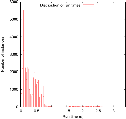
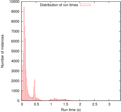
Figure 10: Distribution of run times for E in automatic mode (left) and using an optimized strategy (right) for the UCLID test set.

These problems (all valid) turned out to be easy for E in automatic mode, where the prover chooses automatically ordering and search plan. It could solve all problems, taking less than 4 sec on the hardest one, with average 0.372 sec and median 0.25 sec. Figure 10 shows a histogram of run times: the vast majority of problems was solved in less than 1 sec and very few needed between 1.5 and 3 sec. An optimized search plan was found by testing on a random sample of 500 problems, or less than 1% of the full set. With this search plan, very similar to E(std-kbo), the performance improved by about 40% (Figure 10, right): the average is 0.249 sec, the median 0.12 sec, the longest time 2.77 sec, and most problems were solved in less than 0.5 sec.

7 Discussion

The application of automated reasoning to verification has long shown the importance of decision procedures for satisfiability in decidable theories. The most common approach to these procedures, popularized as the “little” proof engines paradigm [Shankar (2002)], works by building each theory ${\cal T}$ into a dedicated inference engine. For ${\cal T}$-satisfiability procedures, that decide conjunctions of ground ${\cal T}$-literals, the mainstay is the congruence closure algorithm, enhanced by building ${\cal T}$ into the algorithm (e.g., [Nelson and Oppen (1980), Stump et al. (2001), Lahiri and Musuvathi (2005b), Lahiri and Musuvathi (2005a), Dutertre and de Moura (2006), Nieuwenhuis and Oliveras (2007)]). Such procedures are combined according to the scheme of [Nelson and Oppen (1979)] or its variants (e.g., [Tinelli and Harandi (1996), Barrett et al. (2002b), Ganzinger (2002), Ghilardi (2004), Baader and Ghilardi (2005), Ranise et al. (2005)]). Recent systematic treatments appeared in [Krstić and Conchon (2003), Manna and Zarba (2003), Conchon and Krstić (2003), Ranise et al. (2004), Ganzinger et al. (2004), Ghilardi et al. (2005)].

For ${\cal T}$-decision procedures, that decide arbitrary quantifier-free ${\cal T}$-formulæ, the so-called “eager” approaches seek efficient reductions of the problems to SAT and submit them to SAT solvers (e.g., [Jackson and Vaziri (2000), Bryant and Velev (2001), Bryant et al. (2002), Seshia et al. (2003), Meir and Strichman (2005)]). The so-called “lazy” approaches (e.g., [de Moura et al. (2002), Barrett et al. (2002a), Flanagan et al. (2003), Déharbe and Ranise (2003), Barrett and Berezin (2004), Ganzinger et al. (2004), Detlefs et al. (2005), Bozzano et al. (2005), Bozzano et al. (2005), Nieuwenhuis and Oliveras (2007)]) integrate ${\cal T}$-satisfiability procedures based on congruence closure with SAT solvers, usually based on the Davis-Putnam-Logemann-Loveland procedure (e.g., [Chang and Lee (1973), Moskewicz et al. (2001)]). The resulting systems are called SMT solvers.

By symmetry with little proof engines, we used “big” proof engines (e.g., [Stickel (2002)]), for theorem-proving strategies for full first-order logic with equality, as implemented in state-of-the-art general-purpose theorem provers (e.g., [McCune (2003), Weidenbach et al. (1999), Riazanov and Voronkov (2002), Schulz (2002)]). There has always been a continuum between big and little engines of proof, as testified by the research on reasoning modulo a theory in big engines. The rewriting approach to ${\cal T}$-satisfiability aims at a cross-fertilization where big engines work as little engines. The general idea is to explore how the technology of big engines (orderings, inference rules, search plans, algorithms, data structures, implementation techniques) may be applied selectively and efficiently “in the small,” that is, to decide specific theories.

This exploration finds its historical roots in the relationship between congruence closure and Knuth-Bendix completion [Knuth and Bendix (1970)] in the ground case: the application of ground completion to compute congruence closure was discovered as early as [Lankford (1975)]; the usage of congruence closure to generate canonical rewrite systems from sets of ground equations was investigated further in [Gallier et al. (1993), Plaisted and Sattler-Klein (1996)]; more recently, a comparison of ground completion and congruence closure algorithms was given in [Bachmair et al. (2003)]; and ground completion and congruence closure were included in an abstract framework for canonical inference in [Bonacina and Dershowitz (2007)]. The central component of the rewriting approach is the inference system $\cal SP$, that is an offspring of a long series of studies on completion for first-order logic with equality. These systems were called by various authors rewrite-based, completion-based, superposition-based, paramodulation-based, contraction-based, saturation-based or ordering-based, to emphasize one aspect or the other. Relevant surveys include [Plaisted (1993), Bonacina (1999), Nieuwenhuis and Rubio (2001), Dershowitz and Plaisted (2001)].

The gist of the rewriting approach to ${\cal T}$-satisfiability is to show that a sound and refutationally complete “big” engine, such as $\cal SP$, is guaranteed to generate finitely many clauses from ${\cal T}$-satisfiability problems. By adding termination to soundness and completeness, one gets a decision procedure: an $\cal SP$-strategy that combines $\cal SP$ with a fair search plan is a ${\cal T}$-satisfiability procedure. Depending on the theory, termination may require some problem transformation, termed ${\cal T}$-reduction, which is fully mechanizable for all the theories we have studied. We emphasize that the inference system is not adapted to the theories. The only requirement is on the ordering: $\cal SP$ is parametric with respect to a CSO, and the termination proof for ${\cal T}$ may require that this ordering satisfies some property named ${\cal T}$-goodness. For all considered theories, ${\cal T}$-goodness is very simple and easily satisfied by common orderings such as RPO’s and KBO’s.

We proved termination of $\cal SP$ on several new theories, including one with infinite axiomatization. We gave a general modularity theorem for the combination of theories, and carried out an experimental evaluation, to test the pratical feasibility of the rewriting approach. The modularity theorem states sufficient conditions (no shared function symbols, variable-inactive theories) for $\cal SP$ to terminate on a combination of theories if it terminates on each theory separately. The “no shared function symbols” hypothesis is common for combination results. Variable-inactivity is satisfied by all equational theories with no trivial models. First-order theories that fail to be variable-inactive in an intuitive way are not stably infinite, and therefore cannot be combined by the Nelson-Oppen scheme either. On the other hand, it follows from work in [Bonacina et al. (2006)] that variable-inactive theories are stably infinite. The quantifier-free theories of equality, lists, arrays with or without extensionality, records with or without extensionality, integer offsets and integer offsets modulo, all satisfy these requirements, so that any fair $\cal SP$-strategy is a satisfiability procedure for any of their combinations. The theories of arrays and possibly empty lists are not convex, and therefore cannot be combined by the Nelson-Oppen scheme without case analysis.

A different approach to big engines in the context of theory reasoning, and especially combination of theories, appeared in [Ganzinger et al. (2006)]: the combination or extension of theories is conceived as mixing total and partial functions, and a new inference system with partial superposition is introduced to handle them. Because the underlying notion of validity is modified to accomodate partial functions, the emphasis of [Ganzinger et al. (2006)] is on defining the new inference system and proving its completeness. The realization of such an approach requires to implement the new inference system. The essence of our methodology, on the other hand, is to leave the inference system and its completeness proof unchanged, and prove termination to get decision procedures. This allows us to take existing theorem provers “off the shelf.”

For the experimental evaluation, we designed six sets of synthetic benchmarks on the theory of arrays with extensionality and combinations of the theories of arrays, records and integer offsets or integer offsets modulo. For “real-world problems,” we considered satisfiability benchmarks extracted from the UCLID suite. Our experimental comparison between the $\cal SP$-based E prover and the validity checkers CVC and CVC Lite is a first of its kind, and offers many elements for reflection and suggestions for future research.

The analysis of the traces of the theorem prover showed that these satisfiability problems behave very differently compared to more typical theorem-proving problems. Classical proof tasks involve a fairly large set of axioms, a rich signature, many universally quantified variables, many unit clauses usable as rewrite rules and many mixed positive/negative literal clauses. The search space is typically infinite, and only a very small part of it gets explored. In ${\cal T}$-satisfiability problems, input presentations are usually very small and there is a large number of ground rewrite rules generated by flattening. The search space is finite, but nearly all of it has to be explored, before unsatisfiability (validity) can be shown. Table 1 compares the behavior of E on some medium-difficulty unsatisfiable array problems and some representative TPTP problems of similar difficulty for the prover.

Problem	Initial	Generated	Processed	Remaining	Unnecessary
Name	clauses	clauses	clauses	clauses	inferences
$\operatorname{{\tt STORECOMM}}(60)/1$	1896	2840	4323	7	26.4%
$\operatorname{{\tt STOREINV}}(5)$	27	22590	7480	31	95.5%
$\operatorname{{\tt SWAP}}(8)/3$	62	73069	21743	56	98.2%
SET015-4	15	39847	7504	16219	99.90%
FLD032-1	31	44192	3964	31642	99.96%
RNG004-1	20	50551	4098	26451	99.90%

The data are for E in automatic mode. $\operatorname{{\tt STORECOMM}}(60)/1$ is one of the problems in $\operatorname{{\tt STORECOMM}}(n)$ for $n=60$, $\operatorname{{\tt STOREINV}}(5)$ is $\operatorname{{\tt STOREINV}}(n)$ for $n=5$ and $\operatorname{{\tt SWAP}}(8)/3$ is one of the problems in $\operatorname{{\tt SWAP}}(n)$ for $n=8$. The others are representative problems from TPTP 3.0.0. The sum of processed and remaining clauses may be smaller than the sum of initial and generated clauses, because E removes newly generated trivial clauses, as well as unprocessed clauses whose parents become redundant, without counting them as processed. The final column shows the percentage of all inferences (expansion and contraction) that did not contribute to the final proof.

Table 1: Performance characteristics of array and TPTP problems.

Most search plans and features of first-order provers were designed assuming the search space characteristics of typical first-order problems. Thus, the theorem prover turned out to be competitive with the little-engines systems, although it was optimized for different search problems. This means that not only is using a theorem prover already a viable option in practice, but there is a clear potential to improve both performance and usability, by studying implementation techniques of first-order inferences that target ${\cal T}$-satisfiability, by designing theory-specific search plans, and by equipping the prover with the ability to recognize which theories appear in the input set. The prover also terminated in many cases beyond the known termination results (cf. Figure 6 and the runs with E(std-kbo), whose ordering is not ${\cal A}$-good). Thus, theorem provers are not as brittle as one may fear with respect to termination, and still offer the flexibility of adding useful lemmata to the presentation, as shown in Section 6.2.

The above remarks suggest that stronger termination results may be sought. The complexity of the rewrite-based procedures may be improved by adopting theory-specific search plans. Methods to extract models from saturated sets can be investigated to complement proof finding with model generation, which is important for applications. For instance, in verification, a model represents a counter-example to a conjecture of correctness of a system. The ability to generate models marks the difference between being able to tell that there are errors (by reporting “satisfiable”), and being able to give some information on the errors (by reporting “satisfiable” and a model). Since we do not expect the rewrite-based approach to work for full linear arithmetic, another quest is how to integrate it with methods for arithmetic [Rueß and Shankar (2004)] or other theories such as bit-vectors [Cyrluk et al. (1996)]. Research on integration with the latter theory began in [Kirchner et al. (2005)].

Most verification problems involve arbitrary quantifier-free ${\cal T}$-formulæ, or, equivalently, sets of ground ${\cal T}$-clauses. Thus, a major open issue is how to apply big engines towards solving general ${\cal T}$-decision problems. Since $\cal SP$ is an inference system for general first-order clauses, a set of ground ${\cal T}$-clauses may be submitted to an $\cal SP$-based prover. Showing that an $\cal SP$-strategy is a ${\cal T}$-decision procedure requires extending the termination results from sets of ground literals to sets of ground clauses. Sufficient conditions for termination of $\cal SP$ on ${\cal T}$-decision problems were given recently in [Bonacina and Echenim (2007a)]. However, verification problems of practical interest typically yield large sets with huge non-unit clauses, and first-order provers are not designed to deal with large disjunctions as efficiently as SAT solvers.

In practice, a more plausible approach could be to follow a simple “lazy” scheme (e.g., [Barrett et al. (2002a), Flanagan et al. (2003)]), and integrate a rewrite-based ${\cal T}$-satisfiability procedure with a SAT solver that generates assignments. The rewrite-based ${\cal T}$-solver produces a proof, whenever it detects unsatisfiability, and can be made incremental to interact with the SAT solver according to the “lazy” scheme. However, the state of the art in SMT solvers indicates that a tight integration of the two solvers is required to achieve high performances. SAT solvers are based on case analysis by backtracking, whereas rewrite-based inference engines are proof-confluent, which means they need no backtracking. While proof confluence is an advantage in first-order theorem proving, this dissimilarity means that a tight integration of SAT solver and rewrite-based ${\cal T}$-solver requires to address the issues posed by the interplay of two very different kinds of control.

In current work we are taking a diffrent route: we are exploring ways to decompose ${\cal T}$-decision problems, in such a way that the big engine acts as a pre-processor for an SMT solver, doing as much theory reasoning as possible in the pre-processing phase. In this way we hope to combine the strength of a prover, such as E, in equational reasoning with that of an SMT solver in case analysis. Even more general problems require to reason with universally quantified variables, that SMT solvers handle only by heuristics, following the historical lead of [Detlefs et al. (2005)]. In summary, big engines are strong at reasoning with equalities, universally quantified variables and Horn clauses. Little engines are strong at reasoning with propositional logic, non-Horn clauses and arithmetic. The reasoning environments of the future will have to harmonize their forces.

We are indebted to Mnacho Echenim for several suggestions to improve preliminary versions of this paper, and especially for helping us correcting the proofs of Section 3.2.

eceived April 2006
Revised February 2007
Accepted June 2007

References

- Arkoudas et al. (2004) Arkoudas, K., Zee, K., Kuncak, V., and Rinard, M. 2004. Verifying a file system implementation. In Proc. 6th ICFEM, J. Davies, W. Schulte, and M. Barnett, Eds. LNCS, vol. 3308. Springer, 373–390.
- Armando et al. (2002) Armando, A., Bonacina, M. P., Ranise, S., Rusinowitch, M., and Sehgal, A. K. 2002. High-performance deduction for verification: a case study in the theory of arrays. In Notes 2nd VERIFY Workshop, 3rd FLoC. Number 07/2002 in Technical Reports. DIKU, U. Copenhagen, 103–112.
- Armando et al. (2005a) Armando, A., Bonacina, M. P., Ranise, S., and Schulz, S. 2005a. Big proof engines as little proof engines: new results on rewrite-based satisfiability procedures. In Notes 3rd PDPAR Workshop, CAV-17. 33–41.
- Armando et al. (2005b) Armando, A., Bonacina, M. P., Ranise, S., and Schulz, S. 2005b. On a rewriting approach to satisfiability procedures: extension, combination of theories and an experimental appraisal. In Proc. 5th FroCoS, B. Gramlich, Ed. LNAI, vol. 3717. Springer, 65–80.
- Armando et al. (2003) Armando, A., Ranise, S., and Rusinowitch, M. 2003. A rewriting approach to satisfiability procedures. Information and Computation 183, 2, 140–164.
- Baader and Ghilardi (2005) Baader, F. and Ghilardi, S. 2005. Connecting many-sorted structures and theories through adjoint functions. In Proc. 5th FroCoS, B. Gramlich, Ed. LNAI, vol. 3717. Springer, 31–47.
- Bachmair et al. (2003) Bachmair, L., Tiwari, A., and Vigneron, L. 2003. Abstract congruence closure. J. of Automated Reasoning 31, 2, 129–168.
- Barrett and Berezin (2004) Barrett, C. W. and Berezin, S. 2004. CVC Lite: a new implementation of the Cooperating Validity Checker. In Proc. CAV-16, R. Alur and D. A. Peled, Eds. LNCS, vol. 3114. Springer, 515–518.
- Barrett et al. (2000) Barrett, C. W., Dill, D. L., and Stump, A. 2000. A framework for cooperating decision procedures. In Proc. CADE-17, D. McAllester, Ed. LNAI, vol. 1831. Springer, 79–97.
- Barrett et al. (2002a) Barrett, C. W., Dill, D. L., and Stump, A. 2002a. Checking satisfiability of first-order formulas by incremental translation to SAT. In Proc. CAV-14, K. G. Larsen and E. Brinksma, Eds. LNCS, vol. 2404. Springer, 236–249.
- Barrett et al. (2002b) Barrett, C. W., Dill, D. L., and Stump, A. 2002b. A generalization of Shostak’s method for combining decision procedures. In Proc. 4th FroCoS, A. Armando, Ed. LNCS, vol. 2309. Springer.
- Bonacina (1999) Bonacina, M. P. 1999. A taxonomy of theorem-proving strategies. In Artificial Intelligence Today – Recent Trends and Developments, M. J. Wooldridge and M. Veloso, Eds. LNAI, vol. 1600. Springer, 43–84.
- Bonacina and Dershowitz (2007) Bonacina, M. P. and Dershowitz, N. 2007. Abstract canonical inference. ACM Trans. on Computational Logic 8, 1 (January), 180–208.
- Bonacina and Echenim (2007a) Bonacina, M. P. and Echenim, M. 2007a. Rewrite-based decision procedures. In Proc. 6th STRATEGIES Workshop, FLoC 2006, M. Archer, T. B. de la Tour, and C. Munoz, Eds. ENTCS, vol. 174(11). Elsevier, 27–45.
- Bonacina and Echenim (2007b) Bonacina, M. P. and Echenim, M. 2007b. Rewrite-based satisfiability procedures for recursive data structures. In Proc. 4th PDPAR Workshop, FLoC 2006, B. Cook and R. Sebastiani, Eds. ENTCS, vol. 174(8). Elsevier, 55–70.
- Bonacina et al. (2006) Bonacina, M. P., Ghilardi, S., Nicolini, E., Ranise, S., and Zucchelli, D. 2006. Decidability and undecidability results for Nelson-Oppen and rewrite-based decision procedures. In Proc. IJCAR-3, U. Furbach and N. Shankar, Eds. LNAI, vol. 4130. Springer, 513–527.
- Bonacina and Hsiang (1995) Bonacina, M. P. and Hsiang, J. 1995. Towards a foundation of completion procedures as semidecision procedures. Theoretical Computer Science 146, 199–242.
- Bozzano et al. (2005) Bozzano, M., Bruttomesso, R., Cimatti, A., Junttila, T., Ranise, S., Sebastiani, R., and van Rossum, P. 2005. Efficient satisfiability modulo theories via delayed theory combination. In Proc. CAV-17, K. Etessami and S. Rajamani, Eds. LNCS, vol. 3576. Springer, 335–349.
- Bozzano et al. (2005) Bozzano, M., Bruttomesso, R., Cimatti, A., Junttila, T., van Rossum, P., Schulz, S., and Sebastiani, R. 2005. MathSAT: Tight integration of SAT and mathematical decision procedures. J. of Automated Reasoning 35, 1–3, 265–293.
- Bryant et al. (2002) Bryant, R. E., Lahiri, S. K., and Seshia, S. A. 2002. Modeling and verifying systems using a logic of counter arithmetic with lambda expressions and uninterpreted functions. In Proc. CAV-14, K. G. Larsen and E. Brinksma, Eds. LNCS, vol. 2404. Springer, 78–92.
- Bryant and Velev (2001) Bryant, R. E. and Velev, M. N. 2001. Processor verification using efficient reductions of the logic of uninterpreted functions to propositional logic. ACM Trans. on Computational Logic 2, 1, 93–134.
- Caferra et al. (2004) Caferra, R., Leitsch, A., and Peltier, N. 2004. Automated Model Building. Kluwer Academic Publishers.
- Chang and Lee (1973) Chang, C.-L. and Lee, R. C.-T. 1973. Symbolic Logic and Mechanical Theorem Proving. Academic Press.
- Conchon and Krstić (2003) Conchon, S. and Krstić, S. 2003. Strategies for combining decision procedures. In Proc. TACAS-9, H. Garavel and J. Hatcliff, Eds. LNCS, vol. 2619. Springer, 537–553.
- Cyrluk et al. (1996) Cyrluk, D., Lincoln, P., and Shankar, N. 1996. On Shostak’s decision procedure for combination of theories. In Proc. CADE-13, M. A. McRobbie and J. K. Slaney, Eds. LNAI, vol. 1104. Springer, 463–477.
- Cyrluk et al. (1996) Cyrluk, D., Möller, O., and Rueß, H. 1996. An efficient decision procedure for a theory of fixed-sized bitvectors with composition and extraction. Tech. Rep. UIB96-08, Fakultät für Informatik, Universität Ulm, Ulm, Germany.
- de Moura et al. (2004) de Moura, L., Owre, S., Rueß, H., Rushby, J., and Shankar, N. 2004. The ICS decision procedures for embedded deduction. In Proc. IJCAR-2, D. Basin and M. Rusinowitch, Eds. LNAI, vol. 3097. Springer, 218–222.
- de Moura et al. (2002) de Moura, L., Rueß, H., and Sorea, M. 2002. Lazy theorem proving for bounded model checking over infinite domains. In Proc. CADE-18, A. Voronkov, Ed. LNAI, vol. 2392. Springer, 438–455.
- Déharbe and Ranise (2003) Déharbe, D. and Ranise, S. 2003. Light-weight theorem proving for debugging and verifying units of code. In Proc. 1st SEFM. IEEE Computer Society Press, 220–228.
- Dershowitz (1991) Dershowitz, N. 1991. A maximal-literal unit strategy for Horn clauses. In Proc. CTRS-90, S. Kaplan and M. Okada, Eds. LNCS, vol. 516. Springer, 14–25.
- Dershowitz and Plaisted (2001) Dershowitz, N. and Plaisted, D. A. 2001. Rewriting. In Handbook of Automated Reasoning, A. Robinson and A. Voronkov, Eds. Vol. 1. Elsevier, 535–610.
- Detlefs et al. (2005) Detlefs, D. L., Nelson, G., and Saxe, J. B. 2005. Simplify: a theorem prover for program checking. J. ACM 52, 3, 365–473.
- Downey et al. (1978) Downey, P. J., Samet, H., and Sethi, R. 1978. Off-line and on-line algorithms for deducing equalities. In Proc. POPL-5. ACM Press, 158–170.
- Downey et al. (1980) Downey, P. J., Sethi, R., and Tarjan, R. E. 1980. Variations on the common subexpression problem. J. ACM 27, 4, 758–771.
- Dutertre and de Moura (2006) Dutertre, B. and de Moura, L. 2006. A fast linear-arithmetic solver for DPLL(T). In Proc. CAV-18, T. Ball and R. B. Jones, Eds. LNCS, vol. 4144. Springer, 81–94.
- Fermüller et al. (2001) Fermüller, C., Leitsch, A., Hustadt, U., and Tammet, T. 2001. Resolution decision procedures. In Handbook of Automated Reasoning, A. Robinson and A. Voronkov, Eds. Vol. 2. Elsevier, Chapter 25, 1793–1849.
- Flanagan et al. (2003) Flanagan, C., Joshi, R., Ou, X., and Saxe, J. B. 2003. Theorem proving using lazy proof explication. In Proc. CAV-15, J. Warren A. Hunt and F. Somenzi, Eds. LNCS, vol. 2725. Springer, 355–367.
- Gallier et al. (1993) Gallier, J., Narendran, P., Plaisted, D. A., Raatz, S., and Snyder, W. 1993. Finding canonical rewriting systems equivalent to a finite set of ground equations in polynomial time. J. ACM 40, 1, 1–16.
- Ganzinger (2002) Ganzinger, H. 2002. Shostak light. In Proc. CADE-18, A. Voronkov, Ed. LNAI, vol. 2392. Springer, 332–347.
- Ganzinger et al. (2004) Ganzinger, H., Hagen, G., Nieuwenhuis, R., Oliveras, A., and Tinelli, C. 2004. DPLL(T): Fast decision procedures. In Proc. CAV-16, R. Alur and D. A. Peled, Eds. LNCS, vol. 3114. Springer, 175–188.
- Ganzinger et al. (2004) Ganzinger, H., Rueß, H., and Shankar, N. 2004. Modularity and refinement in inference systems. Tech. Rep. CSL-SRI-04-02, SRI International, Menlo Park, CA, U.S.A.
- Ganzinger et al. (2006) Ganzinger, H., Sofronie, V., and Waldmann, U. 2006. Modular proof systems for partial functions with Evans equality. Information and Computation 240, 10, 1453–1492.
- Ghilardi (2004) Ghilardi, S. 2004. Model-theoretic methods in combined constraint satisfiability. J. of Automated Reasoning 33, 3-4, 221–249.
- Ghilardi et al. (2005) Ghilardi, S., Nicolini, E., and Zucchelli, D. 2005. A comprehensive framework for combined decision procedures. In Proc. 5th FroCoS, B. Gramlich, Ed. LNAI, vol. 3717. Springer, 1–30.
- Horn (1951) Horn, A. 1951. On sentences which are true of direct unions of algebras. Journal of Symbolic Logic 16, 14–21.
- Jackson and Vaziri (2000) Jackson, D. and Vaziri, M. 2000. Finding bugs with a constraint solver. In Proc. ISSTA 2000, M. J. Harrold, Ed. ACM SIGSOFT.
- Kaufmann et al. (2000) Kaufmann, M., Manolios, P., and Moore, Eds., J. S. 2000. Computer Aided Reasoning : ACL2 Case Studies. Kluwer.
- Kirchner et al. (2005) Kirchner, H., Ranise, S., Ringeissen, C., and Tran, D. K. 2005. On superposition-based satisfiability procedures and their combination. In Proc. 2nd ICTAC, D. Hung and M. Wirsing, Eds. LNCS, vol. 3722. Springer, 594–608.
- Knuth and Bendix (1970) Knuth, D. E. and Bendix, P. B. 1970. Simple word problems in universal algebras. In Computational Problems in Abstract Algebra, J. Leech, Ed. Pergamon Press, Oxford, 263–297.
- Krstić and Conchon (2003) Krstić, S. and Conchon, S. 2003. Canonization for disjoint unions of theories. In Proc. CADE-19, F. Baader, Ed. LNCS, vol. 2741. Springer.
- Lahiri and Musuvathi (2005a) Lahiri, S. K. and Musuvathi, M. 2005a. An efficient decision procedure for UTVPI constraints. In Proc. 5th FroCoS, B. Gramlich, Ed. LNAI, vol. 3717. Springer, 168–183.
- Lahiri and Musuvathi (2005b) Lahiri, S. K. and Musuvathi, M. 2005b. An efficient Nelson-Oppen decision procedure for difference constraints over rationals. In Notes 3rd PDPAR Workshop, CAV-17. 2–9.
- Lahiri and Seshia (2004) Lahiri, S. K. and Seshia, S. A. 2004. The UCLID decision procedure. In Proc. CAV-16, R. Alur and D. A. Peled, Eds. LNCS, vol. 3114. Springer, 475–378.
- Lankford (1975) Lankford, D. S. 1975. Canonical inference. Memo ATP-32, Automatic Theorem Proving Project, University of Texas, Austin, TX, U.S.A.
- Lynch and Morawska (2002) Lynch, C. and Morawska, B. 2002. Automatic decidability. In Proc. LICS-17, G. Plotkin, Ed. IEEE Computer Society Press.
- Lynch and Tran (2007) Lynch, C. and Tran, D.-K. 2007. Automatic decidability and combinability revisited. In Proc. CADE-21, F. Pfenning, Ed. LNAI, vol. 4603. Springer, 328–344.
- Manna and Zarba (2003) Manna, Z. and Zarba, C. G. 2003. Combining decision procedures. In Formal methods at the crossroads: from panacea to foundational support. LNCS, vol. 2757. Springer, 381–422.
- McCune (2003) McCune, W. W. 2003. Otter 3.3 reference manual. Tech. Rep. ANL/MCS-TM-263, MCS Division, Argonne National Laboratory, Argonne, IL, U.S.A.
- Meir and Strichman (2005) Meir, O. and Strichman, O. 2005. Yet another decision procedure for equality logic. In Proc. CAV-17, K. Etessami and S. Rajamani, Eds. LNCS, vol. 3576. Springer, 307–320.
- Moskewicz et al. (2001) Moskewicz, M. W., Madigan, C. F., Zhao, Y., Zhang, L., and Malik, S. 2001. Chaff: Engineering an efficient SAT solver. In Proc. 39th DAC, D. Blaauw and L. Lavagno, Eds. ACM Press, 530–535.
- Necula and Lee (1998) Necula, G. and Lee, P. 1998. Efficient representation and validation of proofs. In Proc. LICS-13, V. Pratt, Ed. IEEE Computer Society Press, 93–104.
- Nelson and Oppen (1979) Nelson, G. and Oppen, D. C. 1979. Simplification by cooperating decision procedures. ACM TOPLAS 1, 2, 245–257.
- Nelson and Oppen (1980) Nelson, G. and Oppen, D. C. 1980. Fast decision procedures based on congruence closure. J. ACM 27, 2, 356–364.
- Nieuwenhuis and Oliveras (2007) Nieuwenhuis, R. and Oliveras, A. 2007. Fast congruence closure and extensions. Information and Computation 205, 4, 557–580.
- Nieuwenhuis and Rubio (2001) Nieuwenhuis, R. and Rubio, A. 2001. Paramodulation-based theorem proving. In Handbook of Automated Reasoning, A. Robinson and A. Voronkov, Eds. Vol. 1. Elsevier, 371–443.
- Oppen (1980) Oppen, D. C. 1980. Reasoning about recursively defined data structures. J. ACM 27, 3.
- Owre et al. (1992) Owre, S., Rushby, J. M., and Shankar, N. 1992. PVS: a prototype verification system. In Proc. CADE-11, D. Kapur, Ed. LNAI, vol. 607. Springer, 748–752.
- Plaisted (1993) Plaisted, D. A. 1993. Equational reasoning and term rewriting systems. In Handbook of Logic in Artificial Intelligence and Logic Programming, C. J. H. Dov M. Gabbay and J. A. Robinson, Eds. Vol. I: Logical Foundations. Oxford University Press, 273–364.
- Plaisted and Sattler-Klein (1996) Plaisted, D. A. and Sattler-Klein, A. 1996. Proof lengths for equational completion. Information and Computation 125, 2, 154–170.
- Ranise and Déharbe (2003) Ranise, S. and Déharbe, D. 2003. Light-weight theorem proving for debugging and verifying pointer manipulating programs. In Proc. FTP-2003, I. Dahn and L. Vigneron, Eds. Number DSCI–II710/03 in Technical Reports. Universidad Politécnica de Valencia, 119–132.
- Ranise et al. (2004) Ranise, S., Ringeissen, C., and Tran, D. K. 2004. Nelson-Oppen, Shostak and the extended canonizer: a family picture with a newborn. In Proc. 1st ICTAC, K. Araki and Z. Liu, Eds. LNCS. Springer.
- Ranise et al. (2005) Ranise, S., Ringeissen, C., and Zarba, C. G. 2005. Combining data structures with nonstably infinite theories using many-sorted logic. In Proc. 5th FroCoS, B. Gramlich, Ed. LNAI, vol. 3717. Springer, 48–64.
- Riazanov and Voronkov (2002) Riazanov, A. and Voronkov, A. 2002. The design and implementation of VAMPIRE. J. of AI Communications 15, 2/3, 91–110.
- Rueß (2004) Rueß, H. 2004. Personal communication on ICS 2.0 (e-mail message to Alessandro Armando).
- Rueß and Shankar (2001) Rueß, H. and Shankar, N. 2001. Deconstructing Shostak. In Proc. LICS-16, J. Halpern, Ed. IEEE Computer Society Press.
- Rueß and Shankar (2004) Rueß, H. and Shankar, N. 2004. Solving linear arithmetic constraints. Tech. Rep. CSL-SRI-04-01, SRI International, Menlo Park, CA, U.S.A.
- Schulz (2002) Schulz, S. 2002. E – a brainiac theorem prover. J. of AI Communications 15, 2–3, 111–126.
- Schulz (2004) Schulz, S. 2004. System description: E 0.81. In IJCAR-2, D. Basin and M. Rusinowitch, Eds. LNAI, vol. 3097. Springer, 2223–228.
- Schulz and Bonacina (2005) Schulz, S. and Bonacina, M. P. 2005. On handling distinct objects in the superposition calculus. In Notes 5th IWIL Workshop, LPAR-11. 66–77.
- Seshia et al. (2003) Seshia, S. A., Lahiri, S. K., and Bryant, R. E. 2003. A hybrid SAT-based decision procedure for separation logic with uninterpreted functions. In Proc. 40th DAC, L. Fix and L. Lavagno, Eds. 425–430.
- Shankar (2002) Shankar, N. 2002. Little engines of proof. Invited talk, 3rd FLoC, Copenhagen, Denmark; and course notes of Fall 2003, http://www.csl.sri.com/users/shankar/LEP.html.
- Shostak (1978) Shostak, R. E. 1978. An algorithm for reasoning about equality. C. ACM 21, 7, 583–585.
- Shostak (1984) Shostak, R. E. 1984. Deciding combinations of theories. J. ACM 31, 1, 1–12.
- Stickel (2002) Stickel, M. E. 2002. Herbrand Award speech. 3rd FLoC, Copenhagen, Denmark.
- Stump (2005) Stump, A. 2005. Personal communication on CVC 1.0a (e-mail message to Alessandro Armando).
- Stump et al. (2002) Stump, A., Barrett, C. W., and Dill, D. L. 2002. CVC: a Cooperating Validity Checker. In Proc. CAV-14, K. G. Larsen and E. Brinksma, Eds. LNCS, vol. 2404. Springer, 500–504.
- Stump et al. (2001) Stump, A., Barrett, C. W., Dill, D. L., and Levitt, J. 2001. A decision procedure for an extensional theory of arrays. In Proc. LICS-16, J. Halpern, Ed. IEEE Computer Society Press.
- Stump and Dill (2002) Stump, A. and Dill, D. L. 2002. Faster proof checking in the Edinburgh Logical Framework. In Proc. CADE-18, A. Voronkov, Ed. LNAI, vol. 2392. Springer, 392–407.
- Tinelli and Harandi (1996) Tinelli, C. and Harandi, M. 1996. A new correctness proof of the Nelson-Oppen combination procedure. In Proc. 1st FroCoS, F. Baader and K. Schulz, Eds. Applied Logic Series, vol. 3. Kluwer Academic Publishers.
- van Dalen (1989) van Dalen, D. 1989. Logic and Structure. Springer-Verlag. Second edition.
- Weidenbach et al. (1999) Weidenbach, C., Afshordel, B., Brahm, U., Cohrs, C., Engel, T., Keen, E., Theobalt, C., and Topić, D. 1999. System description: Spass version 1.0.0. In Proc. CADE-16, H. Ganzinger, Ed. LNAI, vol. 1632. Springer, 378–382.