An $O(n^{3})$-Time Algorithm for Tree Edit Distance

Abstract

The edit distance between two ordered trees with vertex labels is the minimum cost of transforming one tree into the other by a sequence of elementary operations consisting of deleting and relabeling existing nodes, as well as inserting new nodes. In this paper, we present a worst-case $O(n^{3})$-time algorithm for this problem, improving the previous best $O(n^{3}\log n)$-time algorithm [6]. Our result requires a novel adaptive strategy for deciding how a dynamic program divides into subproblems (which is interesting in its own right), together with a deeper understanding of the previous algorithms for the problem. We also prove the optimality of our algorithm among the family of decomposition strategy algorithms—which also includes the previous fastest algorithms—by tightening the known lower bound of $\Omega(n^{2}\log^{2}n)$ [4] to $\Omega(n^{3})$, matching our algorithm’s running time. Furthermore, we obtain matching upper and lower bounds of $\Theta(nm^{2}(1+\log\frac{n}{m}))$ when the two trees have different sizes $m$ and $n$, where $m<n$.

1 Introduction

The problem of comparing trees occurs in diverse areas such as structured text databases like XML, computer vision, compiler optimization, natural language processing, and computational biology [1, 2, 7, 9, 10].

As an example, we describe an application in computational biology. Ribonucleic acid (RNA) is a polymer consisting of a sequence of nucleotides (Adenine, Cytosine, Guanine, and Uracil) connected linearly via a backbone. In addition, complementary nucleotides (A–U, G–C, and G–U) can form hydrogen bonds, leading to a structural formation called the secondary structure of the RNA. Because of the nested nature of these hydrogen bonds, the secondary structure of RNA can be represented by a rooted ordered tree, as shown in Fig. 1. Recently, comparing RNA sequences has gained increasing interest thanks to numerous discoveries of biological functions associated with RNA. A major fraction of RNA’s function is determined by its secondary structure [8]. Therefore, computing the similarity between the secondary structure of two RNA molecules can help determine the functional similarities of these molecules.

Figure 1: Two different ways of viewing an RNA sequence. In (a), a schematic 2-dimensional description of an RNA folding. In (b), the RNA as a rooted ordered tree.

The tree edit distance metric is a common similarity measure for ordered trees, introduced by Tai in the late 1970’s [10] as a generalization of the well-known string edit distance problem [12]. Let $F$ and $G$ be two rooted trees with a left-to-right order among siblings and where each vertex is assigned a label from an alphabet $\Sigma$. The edit distance between $F$ and $G$ is the minimum cost of transforming $F$ into $G$ by a sequence of elementary operations consisting of deleting and relabeling existing nodes, as well as inserting new nodes (allowing at most one operation to be performed on each node). These operations are illustrated in Fig. 2. The cost of elementary operations is given by two functions, $c_{{}_{\mathrm{{del}}}}$ and $c_{{}_{\mathrm{{rel}}}}$, where $c_{{}_{\mathrm{{del}}}}(\tau)$ is the cost of deleting or inserting a vertex with label $\tau$, and $c_{{}_{\mathrm{{rel}}}}(\tau_{1},\tau_{2})$ is the cost of changing the label of a vertex from $\tau_{1}$ to $\tau_{2}$. A deletion in $F$ is equivalent to an insertion in $G$ and vice versa, so we can focus on finding the minimum cost of a sequence of deletions and relabels in both trees that transform $F$ and $G$ into isomorphic trees.

Figure 2: The three editing operations on a tree with vertex labels.

Previous results.

To state running times, we need some basic notation. Let $n$ and $m$ denote the sizes $|F|$ and $|G|$ of the two input trees, ordered so that $n\geq m$. Let $n_{\mathrm{leaves}}$ and $m_{\mathrm{leaves}}$ denote the corresponding number of leaves in each tree, and let $n_{0}pt$ and $m_{0}pt$ denote the corresponding height of each tree, which can be as large as $n$ and $m$ respectively.

Tai [10] presented the first algorithm for computing tree edit distance, which requires $O(n_{\mathrm{leaves}}^{2}m_{\mathrm{leaves}}^{2}nm)$ time and space. Tai’s algorithm thus has a worst-case running time of $O(n^{3}m^{3})=O(n^{6})$. Shasha and Zhang [9] improved this result to an $O(\min\{n_{0}pt,n_{\mathrm{leaves}}\}\cdot\min\{m_{0}pt,m_{\mathrm{leaves}}\}\cdot nm)$ time algorithm using $O(nm)$ space. In the worst case, their algorithm runs in $O(n^{2}m^{2})=O(n^{4})$ time. Klein [6] improved this result to a worst-case $O(m^{2}n\log n)=O(n^{3}\log n)$-time algorithm that uses $O(nm)$ space. In addition, Klein’s algorithm can be adapted to solve an unrooted version of the problem. These last two algorithms are based on closely related dynamic programs, and both present different ways of computing only a subset of a larger dynamic program table; these entries are referred to as relevant subproblems. In [4], Dulucq and Touzet introduced the notion of a decomposition strategy (see Section 2.3) as a general framework for algorithms that use this type of dynamic program, and proved a lower bound of $\Omega(nm\log n\log m)$ time for any such strategy.

Many other solutions have been developed; see [1, 11] for surveys. The most recent development is by Chen [3], who presented a different approach that uses results on fast matrix multiplication. Chen’s algorithm uses $O(nm+nm_{\mathrm{leaves}}^{2}+n_{\mathrm{leaves}}m_{\mathrm{leaves}}^{2.5})$ time and $O(n+(m+n_{\mathrm{leaves}}^{2})\min\{n_{\mathrm{leaves}},n_{0}pt\})$ space. In the worst case, this algorithm runs in $O(nm^{2.5})=O(n^{3.5})$ time. In general, Klein’s algorithm remained the best in terms of worst-case time complexity.

Our results.

In this paper, we present a new algorithm for tree edit distance that falls into the same decomposition strategy framework of [6, 9, 4]. Our algorithm runs in $O(nm^{2}(1+\log\frac{n}{m}))=O(n^{3})$ worst-case time and $O(nm)$ space, and can be adapted for the case where the trees are not rooted. The corresponding edit script can easily be obtained within the same time and space bounds. We therefore improve upon all known algorithms in the worst-case time complexity. Our approach is based on Klein’s, but whereas the recursion scheme in Klein’s algorithm is determined by just one of the two input trees, in our algorithm the recursion depends alternately on both trees. Furthermore, we prove a worst-case lower bound of $\Omega(nm^{2}(1+\log\frac{n}{m}))$ time on all decomposition strategy algorithms. This bound improves the previous best lower bound of $\Omega(nm\log n\log m)$ time [4], and establishes the optimality of our algorithm among all decomposition strategy algorithms. Our algorithm is simple, making it easy to implement, but both the upper and lower bound proofs require complicated analysis.

Roadmap.

In Section 2 we give simple and unified presentations of the two well-known tree edit algorithms, on which our algorithm is based, and the class of decomposition strategy algorithms. We present and analyze our algorithm in Section 3, and prove the matching lower bound in Section 4. We conclude in section 5.

2 Background and Framework

Both the existing algorithms and ours compute the edit distance of finite ordered $\Sigma$-labeled forests, henceforth forests. The unique empty forest/tree is denoted by $\emptyset$. The vertex set of a forest $F$ is written simply as $F$, as when we speak of a vertex $v\in F$. For any forest $F$ and $v\in F$, $\sigma(v)$ denotes the $\Sigma$-label of $v$, $F_{v}$ denotes the subtree of $F$ rooted at $v$, and $F-v$ denotes the forest obtained from $F$ after deleting $v$. The leftmost and rightmost trees of $F$ are denoted by $L_{F}$ and $R_{F}$ and their roots by $\ell_{F}$ and $r_{F}$. We denote by $F-L_{F}$ the forest obtained from $F$ after deleting the entire leftmost tree $L_{F}$; similarly $F-R_{F}$. A forest obtained from $F$ by a sequence of any number of deletions of the leftmost and rightmost roots is called a subforest of $F$.

Given forests $F$ and $G$ and vertices $v\in F$ and $w\in G$, we write $c_{{}_{\mathrm{{del}}}}(v)$ instead of $c_{{}_{\mathrm{{del}}}}(\sigma(v))$ for the cost of deleting or inserting $v$, and we write $c_{{}_{\mathrm{{rel}}}}(v,w)$ instead of $c_{{}_{\mathrm{{rel}}}}(\sigma(v),\sigma(w))$ for the cost relabeling $v$ to $w$. $\delta(F,G)$ denotes the edit distance between the forests $F$ and $G$.

Because insertion and deletion costs are the same (for a node of a given label), insertion in one forest is tantamount to deletion in the other forest. Therefore, the only edit operations we need to consider are relabels and deletions of nodes in both forests. In the next two sections, we briefly present the algorithms of Shasha and Zhang, and of Klein. Our presentation is inspired by the tree similarity survey of Bille [1], and is essential for understanding our algorithm.

2.1 Shasha and Zhang’s Algorithm [9]

Given two forests $F$ and $G$ of sizes $n$ and $m$ respectively, the following lemma is easy to verify. Intuitively, this lemma says that the two rightmost roots in $F$ and $G$ are either matched with each other or one of them is deleted.

Lemma 1 ([9])

$\delta(F,G)$ can be computed as follows:

1. $\delta(\emptyset,\emptyset)=0$

2. $\delta(F,\emptyset)=\delta(F-r_{F},\emptyset)+c_{{}_{\mathrm{{del}}}}(r_{F})$

3. $\delta(\emptyset,G)=\delta(\emptyset,G-r_{G})+c_{{}_{\mathrm{{del}}}}(r_{G})$

4. $\delta(F,G)=\min\left\{\begin{array}[]{l}\delta(F-r_{F},G)+c_{{}_{\mathrm{{del}}}}(r_{F}),\\ \delta(F,G-r_{G})+c_{{}_{\mathrm{{del}}}}(r_{G}),\vphantom{\Bigg{(}}\\ \delta(R_{F}-r_{F},R_{G}-r_{G})\\ \quad{+}\ \delta(F-R_{F},G-R_{G})\\ \quad{+}\ c_{{}_{\mathrm{{rel}}}}(r_{F},r_{G})\end{array}\right.$

The above lemma yields an $O(m^{2}n^{2})$ dynamic program algorithm: If we index the vertices of the forests $F$ and $G$ according to their postorder traversal position, then entries in the dynamic program table correspond to pairs $(F^{\prime},G^{\prime})$ of subforests $F^{\prime}$ of $F$ and $G^{\prime}$ of $G$ where $F^{\prime}$ contains vertices $\{i_{1},\ldots,j_{1}\}$ and $G^{\prime}$ contains vertices $\{i_{2},\ldots,j_{2}\}$ for some $1\leq i_{1}\leq j_{1}\leq n$ and $1\leq i_{2}\leq j_{2}\leq m$.

However, as we will presently see, only $O(\min\{n_{0}pt,n_{\mathrm{leaves}}\}\cdot\min\{m_{0}pt,m_{\mathrm{leaves}}\}\cdot nm)$ different relevant subproblems are encountered by the recursion computing $\delta(F,G)$. We calculate the number of relevant subforests of $F$ and $G$ independently, where a forest $F^{\prime}$ (respectively $G^{\prime}$) is a relevant subforest of $F$ (respectively $G$) if it shows up in the computation of $\delta(F,G)$. Clearly, multiplying the number of relevant subforests of $F$ and of $G$ is an upper bound on the total number of relevant subproblems.

We focus on counting the number of relevant subforests of $F$. The count for $G$ is similar. First, notice that for every node $v\in F$, $F_{v}-v$ is a relevant subproblem. This is because the recursion allows us to delete the rightmost root of $F$ repeatedly until $v$ becomes the rightmost root; we then match $v$ (i.e., relabel it) and get the desired relevant subforest. A more general claim is stated and proved later on in Lemma 3. We define $\mathrm{keyroots}(F)=\{\textrm{the root of }F\}\cup\{v\in F\mid v\textrm{ has a left sibling}\}$. Every relevant subforest of $F$ is a prefix (with respect to the postorder indices) of $F_{v}-v$ for some node $v\in\mathrm{keyroots}(F)$. If we define $\mathrm{cdepth}(v)$ to be the number of keyroot ancestors of $v$, and $\mathrm{cdepth}(F)$ to be the maximum $\mathrm{cdepth}(v)$ over all nodes $v\in F$, we get that the total number of relevant subforest of $F$ is at most

$$\sum_{\!\!\!\!v\in\mathrm{keyroots}(F)\!\!\!\!}|F_{v}| =\sum_{v\in F}\mathrm{cdepth}(v)$$

$$\leq\sum_{v\in F}\mathrm{cdepth}(F)$$

$$=|F|\mathrm{cdepth}(F).$$

This means that given two trees, $F$ and $G$, of sizes $n$ and $m$ we can compute $\delta(F,G)$ in $O(\mathrm{cdepth}(F)\mathrm{cdepth}(G)mn)$ time. Shasha and Zhang also proved that for any tree $T$ of size $n$, $\mathrm{cdepth}(T)\leq\min\{n_{0}pt,n_{\mathrm{leaves}}\}$, hence the result. In the worst case, this algorithm runs in $O(m^{2}n^{2})=O(n^{4})$ time.

2.2 Klein’s Algorithm [6]

Klein’s algorithm is based on a recursion similar to Lemma 1. Again, we consider forests $F$ and $G$ of sizes $|F|=n\geq|G|=m$. Now, however, instead of recursing always on the rightmost roots of $F$ and $G$, we recurse on the leftmost roots if $|L_{F}|\leq|R_{F}|$ and on the rightmost roots otherwise. In other words, the “direction” of the recursion is determined by the (initially) larger of the two forests. We assume the number of relevant subforests of $G$ is $O(m^{2})$; we have already established that this is an upper bound.

We next show that Klein’s algorithm yields only $O(n\log n)$ relevant subforests of $F$. The analysis is based on a technique called heavy path decomposition introduced by Harel and Tarjan [5]. Briefly: we mark the root of $F$ as light. For each internal node $v\in F$, we pick one of $v$’s children of maximum size and mark it as heavy, and we mark all the other children of $v$ as light. We define $\mathrm{ldepth}(v)$ to be the number of light nodes that are ancestors of $v$ in $F$, and $\mathrm{light}(F)$ as the set of all light nodes in $F$. By [5], for any forest $F$ and vertex $v\in F$, $\mathrm{ldepth}(v)\leq\log|F|+O(1)$. Note that every relevant subforest of $F$ is obtained by some $i\leq|F_{v}|$ many consecutive deletions from $F_{v}$ for some light node $v$. Therefore, the total number of relevant subforests of $F$ is at most

$$\sum_{\!\!\!\!v\in\mathrm{light}(F)\!\!\!\!}|F_{v}| =\sum_{v\in F}\mathrm{ldepth}(v)$$

$$\leq\sum_{v\in F}(\log|F|+O(1))$$

$$=O(|F|\log|F|).$$

Thus, we get an $O(m^{2}n\log n)=O(n^{3}\log n)$ algorithm for computing $\delta(F,G)$.

2.3 The Decomposition Strategy Framework

Both Klein’s and Shasha and Zhang’s algorithms are based on Lemma 1. The difference between them lies in the choice of when to recurse on the rightmost roots and when on the leftmost roots. The family of decomposition strategy algorithms based on this lemma was formalized by Dulucq and Touzet in [4].

Definition 1 (Strategy)

Let $F$ and $G$ be two forests. A strategy is a mapping from pairs $(F^{\prime},G^{\prime})$ of subforests of $F$ and $G$ to $\{\mathsf{left},\mathsf{right}\}$.

Each strategy is associated with a specific set of recursive calls (or a dynamic program algorithm). The strategy of Shasha and Zhang’s algorithm is $S(F^{\prime},G^{\prime})=\mathsf{right}$ for all $F^{\prime},G^{\prime}$. The strategy of Klein’s algorithm is $S(F^{\prime},G^{\prime})=\mathsf{left}$ if $|L_{F^{\prime}}|\leq|R_{F^{\prime}}|$, and $S(F^{\prime},G^{\prime})=\mathsf{right}$ otherwise. Notice that Shasha and Zhang’s strategy does not depend on the input trees, while Klein’s strategy depends only on the larger input tree. Dulucq and Touzet proved a lower bound of $\Omega(mn\log m\log n)$ time for any strategy based algorithm.

3 The Algorithm

In this section we present our algorithm for computing $\delta(F,G)$ given two trees $F$ and $G$ of sizes $|F|=n\geq|G|=m$. The algorithm recursively uses Klein’s strategy in a divide-and-conquer manner to achieve $O(nm^{2}(1+\log\frac{n}{m}))=O(n^{3})$ running time in the worst case. The algorithm’s space complexity is $O(nm)$. We begin with the observation that Klein’s strategy always determines the direction of the recursion according to the $F$-subforest, even in subproblems where the $F$-subforest is smaller than the $G$-subforest. However, it is not straightforward to change this since even if at some stage we decide to switch to Klein’s strategy based on the other forest, we must still make sure that all subproblems previously encountered are entirely solved. At first glance this seems like a real obstacle since apparently we only add new subproblems to those that are already computed.

For clarity we describe the algorithm recursively. A dynamic programming description and a proof of the $O(mn)$ space complexity will appear in the full version of this paper.

For a tree $F$ of size $n$, define the set $\mathrm{TopLight}_{F}$ to be the set of roots of the forest obtained by removing the heavy path of $F$ (i.e., the unique path starting from the root along heavy nodes). Note that $\mathrm{TopLight}_{F}$ is the set of light nodes with $\mathrm{ldepth}$ 1 in $F$ (see the definition of $\mathrm{ldepth}$ in section 2.2). This definition is illustrated in Fig. 3.

Figure 3: A tree $F$ with $n$ nodes. The black nodes belong to the heavy path. The white nodes are in $\mathrm{TopLight}_{F}$, and the size of each subtree rooted at a white node is at most $\frac{n}{2}$.

Note that the following two conditions are always satisfied:

• $\displaystyle\sum_{v\in\mathrm{TopLight}_{F}}|F_{v}|\leq n$.
  This follows from the fact that $F_{v^{\prime}}$ and $F_{v^{\prime\prime}}$ are disjoint for any $v^{\prime},v^{\prime\prime}\in\mathrm{TopLight}_{F}$.

• $|F_{v}|<\frac{n}{2}$ for every $v\in\mathrm{TopLight}_{F}$, since otherwise $v$ would be a heavy node.

The Algorithm.

We compute $\delta(F,G)$ recursively as follows:

1. If $|F|<|G|$, compute $\delta(G,F)$ instead. That is, we order the pair $\{F,G\}$ such that $F$ is always the larger forest.

2. Recursively compute $\delta(F_{v},G)$ for all $v\in\mathrm{TopLight}_{F}$. Note that along the way this computes $\delta(F_{v^{\prime}}-v^{\prime},G_{w}-w)$ for all $v^{\prime}$ not in the heavy path of $F$ and for all $w\in G$.

3. Compute $\delta(F,G)$ using Klein’s strategy (matching and deleting either from the left or from the right according to the larger of $F$ and $G$). Do not recurse into subproblems that were previously computed in step (2).

The correctness of the algorithm follows immediately from the correctness of Klein’s algorithm. The algorithm is evidentally a decomposition strategy algorithm, since for all subproblems, it either deletes or matches the leftmost or rightmost roots.

Time Complexity.

We show that our algorithm has a worst-case runtime of $O(m^{2}n(1+\log\frac{n}{m}))=O(n^{3})$.

We proceed by counting the number of subproblems computed in each step of the algorithm. Let $R(F,G)$ denote the number of relevant subproblems encountered by the algorithm in the course of computing $\delta(F,G)$.

In step (2) we compute $\delta(F_{v},G)$ for all $v\in\mathrm{TopLight}_{F}$. Hence, the number of subproblems encountered in this step is $\sum_{v\in\mathrm{TopLight}_{F}}R(F_{v},G)$.

In step (3) we compute $\delta(F,G)$ using Klein’s strategy. We bound the number of relevant subproblems by multiplying the number of relevant subforests in $F$ and in $G$. For $G$, we count all possible $O(|G|^{2})$ subforests obtained by left and right deletions. Note that for any node $v^{\prime}$ not in the heavy path of $F$, the subproblem obtained by matching $v^{\prime}$ with any node $w$ in $G$ was already computed in step (2). This is because any such $v^{\prime}$ is contained in $F_{v}$ for some $v\in\mathrm{TopLight}_{F}$, so $\delta(F_{v^{\prime}}-v^{\prime},G_{w}-w)$ is computed in the course of computing $\delta(F_{v},G)$ (we prove this formally in Lemma 3). Furthermore, note that in Klein’s algorithm, a node $v$ on the heavy path of $F$ cannot be matched or deleted until the remaining subforest of $F$ is precisely $F_{v}$. At this point, both matching $v$ or deleting $v$ results in the same new relevant subforest $F_{v}-v$. This means that we do not have to consider matchings of nodes when counting the number of relevant subproblems in step (3). It suffices to consider only the $|F|$ subforests obtained by deletions according to Klein’s strategy. Thus, the total number of new subproblems encountered step (3) is bounded by $|G|^{2}|F|$.

We have established that $R(F,G)$ is at most

$$|G|^{2}|F|+\sum_{v\in\mathrm{TopLight}_{F}}R(F_{v},G)\textrm{, if }|F|\geq|G|$$

$$|F|^{2}|G|+\sum_{w\in\mathrm{TopLight}_{G}}R(F,G_{w})\textrm{, if }|F|<|G|$$

We first show, by a crude estimate, that this leads to an $O(n^{3})$ runtime. Later, we analyze the dependency on $m$ and $n$ accurately.

Lemma 2

$R(F,G)\leq 4(|F||G|)^{3/2}$.

Proof

We proceed by induction on $|F|+|G|$. There are two symmetric cases. If $|F|\geq|G|$ then $R(F,G)\leq|G|^{2}|F|+\sum_{v\in\mathrm{TopLight}_{F}}R(F_{v},G)$. Hence, by the inductive assumption,

$$R(F,G) \leq|G|^{2}|F|+\sum_{\!\!\!\!\!\!\!v\in\mathrm{TopLight}_{F}\!\!\!\!\!\!\!}4(|F_{v}||G|)^{3/2}$$

$$\leq|G|^{2}|F|+4|G|^{3/2}\sum_{\!\!\!\!\!\!\!v\in\mathrm{TopLight}_{F}\!\!\!\!\!\!\!}|F_{v}|^{3/2}$$

$$\leq|G|^{2}|F|+\mbox{}$$

$${\phantom{\leq}}\quad\ 4|G|^{3/2}\sum_{\!\!\!\!\!\!\!v\in\mathrm{TopLight}_{F}\!\!\!\!\!\!\!}|F_{v}|\max_{\!\!\!\!\begin{subarray}{c}\mbox{\phantom{-}}\\ \ \ \ \ \ \ \ \ v\in\mathrm{TopLight}_{F}\end{subarray}\!\!\!\!}\!\!\!\!\!\!\!\!\!\!\!\sqrt{|F_{v}|}$$

$$\leq|G|^{2}|F|+4|G|^{3/2}|F|\sqrt{|F|/2}$$

$$=|G|^{2}|F|+2\sqrt{2}(|F||G|)^{3/2}$$

$$\leq 4(|F||G|)^{3/2}.$$

Here we have used facts $(\ast)$ and $(\ast\ast)$ and the fact that $|F|\geq|G|$. The case where $|F|<|G|$ is symmetric. ∎

This crude estimate gives a worst-case runtime of $O(n^{3})$. We now analyze the dependence on $m$ and $n$ more accurately. Along the recursion defining the algorithm, we view step (2) as only making recursive calls, but not producing any relevant subproblems. Rather, every new relevant subproblem is created in step (3) for a unique recursive call of the algorithm. So when we count relevant subproblems, we sum the number of new relevant subproblems encountered in step (3) over all recursive calls to the algorithm.

We define sets $A,B\subseteq F$ as follows:

$$A =\big{\{}a\in\mathrm{light}(F):|F_{a}|\geq m\big{\}}$$

$$B =\big{\{}b\in F{-}A:b\in\mathrm{TopLight}_{F_{a}}\text{ for some }a\in A\big{\}}.$$

Note that the root of $F$ belongs to $A$. We count separately:

1. the relevant subproblems created in just step (3) of recursive calls $\delta(F_{a},G)$ for all $a\in A$, and

2. the relevant subproblems encountered in the entire computation of $\delta(F_{b},G)$ for all $b\in B$ (i.e., $\sum_{b\in B}R(F_{b},G)$).

Together, this counts all relevant subproblems for the original $\delta(F,G)$. To see this, consider the original call $\delta(F,G)$. Certainly, the root of $F$ is in $A$. So all subproblems generated in step (3) of $\delta(F,G)$ are counted in (i). Now consider the recursive calls made in step (2) of $\delta(F,G)$. These are precisely $\delta(F_{v},G)$ for $v\in\mathrm{TopLight}_{F}$. For each $v\in\mathrm{TopLight}_{F}$, notice that $v$ is either in $A$ or in $B$; it is in $A$ if $|F_{v}|\geq m$, and in $B$ otherwise. If $v$ is in $B$, then all subproblems arising in the entire computation of $\delta(F_{v},G)$ are counted in (ii). On the other hand, if $v$ is in $A$, then we are in analogous situation with respect to $\delta(F_{v},G)$ as we were in when we considered $\delta(F,G)$ (i.e., we count separately the subproblems created in step (3) of $\delta(F_{v},G)$ and the subproblems coming from $\delta(F_{u},G)$ for $u\in\mathrm{TopLight}_{F_{v}}$).

Earlier in this section, we saw that the number of subproblems created in step (3) of $\delta(F,G)$ is $|G|^{2}|F|$. In fact, for any $a\in A$, by the same argument, the number of subproblems created in step (3) of $\delta(F_{a},G)$ is $|G|^{2}|F_{a}|$. Therefore, the total number of relevant subproblems of type (i) is $|G|^{2}\sum_{a\in A}|F_{a}|$. For $v\in F$, define $\mathrm{depth}_{A}(v)$ to be the number of ancestors of $v$ that lie in the set $A$. We claim that $\mathrm{depth}_{A}(v)\leq 1+\log\frac{n}{m}$ for all $v\in F$. To see this, consider any sequence $a_{0},\dots,a_{k}$ in $A$ where $a_{i}$ is a descendent of $a_{i-1}$ for all $i\in[1,k]$. Note that $|F_{a_{i}}|\leq\frac{1}{2}|F_{a_{i-1}}|$ for all $i\in[1,k]$ since the $a_{i}$ are light nodes, and note that $|F_{a_{k}}|\geq m$ by the definition of $A$. It follows that $k\leq\log\frac{n}{m}$, i.e., $A$ contains no sequence of descendants of length $>1+\log\frac{n}{m}$. So clearly every $v\in F$ has $\mathrm{depth}_{A}(v)\leq 1+\log\frac{n}{m}$.

We now have the number of relevant subproblems of type (i) as

$$|G|^{2}\sum_{a\in A}|F_{a}| =m^{2}\sum_{v\in F}\mathrm{depth}_{A}(v)$$

$$\leq m^{2}\sum_{v\in F}(1+\log\frac{n}{m})$$

$$=m^{2}n(1+\log\frac{n}{m}).$$

The relevant subproblems of type (ii) are counted by $\sum_{b\in B}R(F_{b},G)$. Using Lemma 2, we have

$$\sum_{b\in B}R(F_{b},G) \leq 4|G|^{3/2}\sum_{b\in B}|F_{b}|^{3/2}$$

$$\leq 4|G|^{3/2}\sum_{b\in B}|F_{b}|\max_{b\in B}\sqrt{|F_{b}|}$$

$$\leq 4|G|^{3/2}|F|\sqrt{m}=4m^{2}n.$$

Here we have used the facts that $|F_{b}|<m$ and $\sum_{b\in B}|F_{b}|\leq|F|$ (since the trees $F_{b}$ are disjoint for different $b\in B$). Therefore, the total number of relevant subproblems for $\delta(F,G)$–and hence the runtime of the algorithm–is at most $m^{2}n(1+\log\frac{n}{m})+4m^{2}n=O(m^{2}n(1+\log\frac{n}{m}))$.

Unrooted Trees.

Our algorithm can be adapted to compute edit distance of unrooted ordered trees. An unrooted ordered tree is an acyclic graph with a cyclic ordering defined on the edges incident on each node in the graph. In the modified algorithm, we arbitrarily choose a root for the larger of the two trees. We change the first recursive level of the algorithm, so that it now computes the edit distance with respect to any possible choice of a root for the smaller tree. This does not change the time complexity since the number of different relevant subforests for a tree of size $m$ is bounded by $m^{2}$ whether we consider a single choice for the root or all possible choices. This idea will be described in detail in the full version of this paper.

4 A Tight Lower Bound for Strategy Algorithms

In this section we present a lower bound on the worst-case runtime of strategy algorithms. We first give a simple proof of an $\Omega(m^{2}n)$ lower bound. In the case where $m=\Theta(n)$, this gives a lower bound of $\Omega(n^{3})$ which shows that our algorithm is worst-case optimal among all strategy-based algorithms. To prove that our algorithm is worst-case optimal for any $m\leq n$, we analyze a more complicated scenario that gives a lower bound of $\Omega(m^{2}n(1+\log{\frac{n}{m}}))$, matching the running time of our algorithm.

In analyzing strategies we will use the notion of a computational path, which corresponds to a specific sequence of recursion calls. Recall that for all subforest-pairs $(F^{\prime},G^{\prime})$, the strategy $S$ determines a direction: either $\mathsf{right}$ or $\mathsf{left}$. The recursion can either delete from $F^{\prime}$ or from $G^{\prime}$ or match. A computational path is the sequence of operations taken according to the strategy in a specific sequence of recursive calls. For convenience, we sometimes describe a computational path by the sequence of subproblems it induces, and sometimes by the actual sequence of operations: either “delete from the $F$-subforest”, “delete from the $G$-subforest”, or “match”.

The following lemma states that every strategy computes the edit distance between every two root-deleted subtrees of $F$ and $G$.

Lemma 3

For any strategy $S$, the pair $(F_{v}{-}v,G_{w}{-}w)$ is a relevant subproblem for all $v\in F$ and $w\in G$.

Proof

First note that a node $v^{\prime}\in F_{v}$ (respectively, $w^{\prime}\in G_{w}$) is never deleted or matched before $v$ (respectively, $w$) is deleted or matched. Consider the following computational path:

• Delete from $F$ until $v$ is either the leftmost or the rightmost root.

• Next, delete from $G$ until $w$ is either the leftmost or the rightmost root.

Let $(F^{\prime},G^{\prime})$ denote the resulting subproblem. There are four cases to consider.

1. $v$ and $w$ are the rightmost (leftmost) roots of $F^{\prime}$ and $G^{\prime}$, and $S(F^{\prime},G^{\prime})=\mathsf{right}$ ($\mathsf{left}$).

   Match $v$ and $w$ to get the desired subproblem.

2. $v$ and $w$ are the rightmost (leftmost) roots of $F^{\prime}$ and $G^{\prime}$, and $S(F^{\prime},G^{\prime})=\mathsf{left}$ ($\mathsf{right}$).

   Note that at least one of $F^{\prime},G^{\prime}$ is not a tree (since otherwise this is case (1)). Delete from one which is not a tree. After a finite number of such deletions we have reduced to case (1), either because $S$ changes direction, or because both forests become trees whose roots are $v,w$.

3. $v$ is the rightmost root of $F^{\prime}$, $w$ is the leftmost root of $G^{\prime}$.

   If $S(F^{\prime},G^{\prime})=\mathsf{left}$, delete from $F^{\prime}$; otherwise delete from $G^{\prime}$. After a finite number of such deletions this reduces to one of the previous cases when one of the forests becomes a tree.

4. $v$ is the leftmost root of $F^{\prime}$, $w$ is the rightmost root of $G^{\prime}$.

   This case is symmetric to (3).∎

We now turn to the $\Omega(m^{2}n)$ lower bound on the number of relevant subproblems for any strategy.

Lemma 4

For any strategy $S$, there exists a pair of trees $(F,G)$ with sizes $n,m$ respectively, such that the number of relevant subproblems is $\Omega(m^{2}n)$.

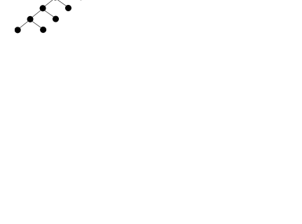
Figure 4: The two trees used to prove an $\Omega(m^{2}n)$ lower bound.

Proof

Let $S$ be an arbitrary strategy, and consider the trees $F$ and $G$ depicted in Fig. 4. According to lemma 3, every pair $(F_{v}{-}v,G_{w}{-}w)$ where $v\in F$ and $w\in G$ is a relevant subproblem for $S$. Focus on such a subproblem where $v$ and $w$ are internal nodes of $F$ and $G$. Denote $v$’s right child by $v_{r}$ and $w$’s left child by $w_{\ell}$. Note that $F_{v}{-}v$ is a forest whose rightmost root is the node $v_{r}$. Similarly, $F_{w}{-}w$ is a forest whose leftmost root is $w_{\ell}$. Starting from $(F_{v}{-}v,G_{w}{-}w)$, consider the computational path $c_{v,w}$ that deletes from $F$ whenever the strategy says $\mathsf{left}$ and deletes from $G$ otherwise. In both cases, neither $v_{r}$ nor $w_{\ell}$ is deleted. Such deletions can be carried out so long as both forests are non-empty.

The length of this computational path is at least $\min\{|F_{v}|,|G_{w}|\}-1$. Note that for each subproblem $(F^{\prime},G^{\prime})$ along this computational path, $v_{r}$ is the rightmost root of $F^{\prime}$ and $w_{\ell}$ is the leftmost root of $G^{\prime}$. It follows that for every two distinct pairs $(v_{1},w_{1})\neq(v_{2},w_{2})$ of internal nodes in $F$ and $G$, the relevant subproblems occurring along the computational paths $c_{v_{1},w_{1}}$ and $c_{v_{2},w_{2}}$ are disjoint. Since there are $\frac{n}{2}$ and $\frac{m}{2}$ internal nodes in $F$ and $G$ respectively, the total number of subproblems along the $c_{v,w}$ computational paths is given by:

$$\sum_{(v,w)\textrm{ internal nodes}}\min\{|F_{v}|,|G_{w}|\}-1 =$$

$$\sum_{i=1}^{\frac{n}{2}}\sum_{j=1}^{\frac{m}{2}}\min\{2i,2j\} =\Omega(m^{2}n)$$

∎

The $\Omega(m^{2}n)$ lower bound established by Lemma 4 is tight if $m=\Theta(n)$, since in this case our algorithm achieves an $O(n^{3})$ runtime.

To establish a tight bound when $m$ is not $\Theta(n)$, we use the following technique for counting relevant subproblems. We associate a subproblem consisting of subforests $(F^{\prime},G^{\prime})$ with the unique pair of vertices $(v,w)$ such that $F_{v},G_{w}$ are the smallest trees containing $F^{\prime},G^{\prime}$ respectively. For example, for nodes $v$ and $w$ with at least two children, the subproblem $(F_{v}{-}v,G_{w}{-}w)$ is associated with the pair $(v,w)$. Note that all subproblems encountered in a computational path starting from $(F_{v}{-}v,G_{w}{-}w)$ until the point where either forest becomes a tree are also associated with $(v,w)$.

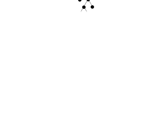
Figure 5: The two trees used to prove $\Omega(m^{2}n\log\frac{n}{m})$ lower bound.

Lemma 5

For every strategy $S$, there exists a pair of trees $(F,G)$ with sizes $n\geq m$ such that the number of relevant subproblems is $\Omega(m^{2}n\log\frac{n}{m})$.

Proof

Consider the trees illustrated in Fig. 5. The $n$-sized tree $F$ is a complete balanced binary tree, and $G$ is a “zigzag” tree of size $m$. Let $w$ be an internal node of $G$ with a single node $w_{r}$ as its right subtree and $w_{\ell}$ as a left child. Denote $m^{\prime}=|G_{w}|$. Let $v$ be a node be a node in $F$ such that $F_{v}$ is a tree of size $n^{\prime}+1$ such that $n^{\prime}\geq 4m\geq 4m^{\prime}$. Denote $v$’s left and right children $v_{\ell}$ and $v_{r}$ respectively. Note that $|F_{v_{\ell}}|=|F_{v_{r}}|=\frac{n^{\prime}}{2}$

Let $S$ be an arbitrary strategy. We aim to show that the total number of relevant subproblems associated with $(v,w)$ or with $(v,w_{\ell})$ is at least $\frac{n^{\prime}m^{\prime}}{4}$. Let $c$ be the computational path that always deletes from $F$ (no matter whether $S$ says $\mathsf{left}$ or $\mathsf{right}$). We consider two complementary cases.

Case 1: $\frac{n^{\prime}}{4}$ left deletions occur in the computational path $c$, and at the time of the $\frac{n^{\prime}}{4}$th left deletion, there were fewer than $\frac{n^{\prime}}{4}$ right deletions.

We define a set of new computational paths $\{c_{j}\}_{1\leq j\leq\frac{n^{\prime}}{4}}$ where $c_{j}$ deletes from $F$ up through the $j$th left deletion, and thereafter deletes from $F$ whenever $S$ says $\mathsf{right}$ and from $G$ whenever $S$ says $\mathsf{left}$. At the time the $j$th left deletion occurs, at least $\frac{n^{\prime}}{4}\geq m^{\prime}-2$ nodes remain in $F_{v_{r}}$ and all $m^{\prime}-2$ nodes are present in $G_{w_{\ell}}$. So on the next $m^{\prime}-2$ steps along $c_{j}$, neither of the subtrees $F_{v_{r}}$ and $G_{w_{\ell}}$ is totally deleted. Thus, we get $m^{\prime}-2$ distinct relevant subproblems associated with $(v,w)$. Notice that in each of these subproblems, the subtree $F_{v_{\ell}}$ is missing exactly $j$ nodes. So we see that, for different values of $j\in[1,\frac{n^{\prime}}{4}]$, we get disjoint sets of $m^{\prime}-2$ relevant subproblems. Summing over all $j$, we get $\frac{n^{\prime}}{4}(m^{\prime}-2)$ distinct relevant subproblems associated with $(v,w)$.

Case 2: $\frac{n^{\prime}}{4}$ right deletions occur in the computational path $c$, and at the time of the $\frac{n^{\prime}}{4}$th right deletion, there were fewer than $\frac{n^{\prime}}{4}$ left deletions.

We define a different set of computational paths $\{\gamma_{j}\}_{1\leq j\leq\frac{n^{\prime}}{4}}$ where $\gamma_{j}$ deletes from $F$ up through the $j$th right deletion, and thereafter deletes from $F$ whenever $S$ says $\mathsf{left}$ and from $G$ whenever $S$ says $\mathsf{right}$ (i.e., $\gamma_{j}$ is $c_{j}$ with the roles of $\mathsf{left}$ and $\mathsf{right}$ exchanged). Similarly as in case 1, for each $j\in[1,\frac{n^{\prime}}{4}]$ we get $m^{\prime}-2$ distinct relevant subproblems in which $F_{v_{r}}$ is missing exactly $j$ nodes. All together, this gives $\frac{n^{\prime}}{4}(m^{\prime}-2)$ distinct subproblems. Note that since we never make left deletions from $G$, the left child of $w_{\ell}$ is present in all of these subproblems. Hence, each subproblem is associated with either $(v,w)$ or $(v,w_{\ell})$.

In either case, we get $\frac{n^{\prime}}{4}(m^{\prime}-2)$ distinct relevant subproblems associated with $(v,w)$ or $(v,w_{\ell})$. To get a lower bound on the number of problems we sum over all pairs $(v,w)$ with $G_{w}$ being a tree whose right subtree is a single node, and $|F_{v}|\geq 4m$. There are $\frac{m}{4}$ choices for $w$ corresponding to tree sizes $4j$ for $j\in[1,\frac{m}{4}]$. For $v$, we consider all nodes of $F$ whose distance from a leaf is at least $\log(4m)$. For each such pair we count the subproblems associated with $(v,w)$ and $(v,w_{\ell})$. So the total number of relevant subproblems counted in this way is

$$\sum_{v,w}\frac{|F_{v}|}{4}(|G_{w}|-2) =\frac{1}{4}\sum_{v}|F_{v}|\sum_{j=1}^{\frac{m}{4}}(4j-2)$$

$$=\frac{1}{4}\sum_{i=\log 4m}^{\log n}\frac{n}{2^{i}}{\cdot}2^{i}\sum_{j=1}^{\frac{m}{4}}(4j-2)$$

$$=\Omega(m^{2}n\log\frac{n}{m})$$

∎

Lemma 6

For every strategy $S$ and $n\geq m$, there exist trees $F$ and $G$ of sizes $\Theta(n)$ and $\Theta(m)$ for which $S$ has $\Omega(m^{2}n(1+\log\frac{n}{m}))$ relevant subproblems.

Proof

If $m=\Theta(n)$ then this bound is $\Omega(m^{2}n)$ as shown in Lemma 4. Otherwise, this bound is $\Omega(m^{2}n\log\frac{n}{m})$ which was shown in Lemma 5. ∎

5 Conclusions

We presented a new $O(n^{3})$-time and $O(n^{2})$-space algorithm for computing the tree edit distance between two ordered trees. Our algorithm is not only faster than all previous algorithms in the worst case, but we have proved it is optimal within the broad class of decomposition strategy algorithms. As a consequence, any future improvements in terms of worst-case time complexity would have to find an entirely new approach. We obtain similar results when considering the sizes $m$ and $n$ of the input trees as separate parameters.

The novelty of our dynamic program is that it is both symmetric in its two inputs as well as adaptively dependant on them. This general notion may also be applied in other scenarios where the known dynamic programming solutions possess an inherent asymmetry.

The full version of the paper includes an explicit dynamic program for our algorithm, a proof of the $O(n^{2})$-space complexity, and an adaptation of the algorithm for the edit distance problem on unrooted trees.

References

- [1] P. Bille. Tree edit distance, alignment distance and inclusion. Technical report TR-2003-23. IT University of Copenhagen, 2003.
- [2] S. S. Chawathe. Comparing hierarchical data in external memory. In Proceedings of the 25th International Conference on Very Large Data Bases, pages 90–101, Edinburgh, Scotland, U.K., 1999.
- [3] W. Chen. New algorithm for ordered tree-to-tree correction problem. 40:135 –158, 2001.
- [4] S. Dulucq and H. Touzet. Analysis of tree edit distance algorithms. In Proceedings of the 14th annual symposium on Combinatorial Pattern Matching (CPM), pages 83–95, 2003.
- [5] D. Harel and R. E. Tarjan. Fast algorithms for finding nearest common ancestors. SIAM Journal of Computing, 13(2):338–355, 1984.
- [6] P. N. Klein. Computing the edit-distance between unrooted ordered trees. In Proceedings of the 6th annual European Symposium on Algorithms (ESA), pages 91–102, 1998.
- [7] P. N. Klein, S. Tirthapura, D. Sharvit, and B. B. Kimia. A tree-edit-distance algorithm for comparing simple, closed shapes. In Proceedings of the 11th ACM-SIAM Symposium on Discrete Algorithms (SODA), pages 696–704, 2000.
- [8] P.B Moore. Structural motifs in RNA. Annual review of biochemistry, 68:287–300, 1999.
- [9] D. Shasha and K. Zhang. Simple fast algorithms for the editing distance between trees and related problems. SIAM Journal of Computing, 18(6):1245–1262, 1989.
- [10] K. Tai. The tree-to-tree correction problem. Journal of the Association for Computing Machinery (JACM), 26(3):422–433, 1979.
- [11] G. Valiente. Algorithms on Trees and Graphs. Springer-Verlag, 2002.
- [12] R. A. Wagner and M. J. Fischer. The string-to-string correction problem. Journal of the ACM, 21(1):168–173, 1974.