Cryptographic Pseudo-Random Sequences from the Chaotic Hénon Map

Abstract

A scheme for pseudo-random binary sequence generation based on the two-dimensional discrete-time Hénon map is proposed. Properties of the proposed sequences pertaining to linear complexity, linear complexity profile, correlation and auto-correlation are investigated. All these properties of the sequences suggest a strong resemblance to random sequences. Results of statistical testing of the sequences are found encouraging. An attempt is made to estimate the keyspace size if the proposed scheme is used for cryptographic applications. The keyspace size is found to be large and is dependent on the precision of the computing platform used.

Keywords: Chaos, nonlinear difference equations, random number generation, stream ciphers, cryptography.

1 Introduction

Pseudo-random number sequences are useful in many applications including monte-carlo simulation, spread spectrum communications, steganography and cryptography. Conventionally, pseudo-random sequence generators based on linear congruential methods and feedback shift-registers are popular [Knuth 1998]. For cryptographic applications, several algorithms such as ANSI X9.17 and FIPS 186 are found to be popular [Menezes et al 1997]. In recent times, several researchers have been exploring the idea of using chaotic dynamical systems for this purpose [Falcioni et al 2006, Kocarev 2001, Woodcock & Smart 1998]. The random-like, unpredictable dynamics of chaotic systems, their inherent determinism and simplicity of realization suggests their potential for exploitation as pseudo-random number generators.

Cryptographic schemes based on chaos have been classified as  1) discrete-time discrete-value schemes  2) discrete-time continuous-value schemes and  3) continuous-time continuous-value schemes [Dachselt & Schwarz 2001]. All conventional cryptographic schemes act on discrete symbols such as bits, integers, characters and symbols and can be grouped into the first category, that of discrete-time discrete-value schemes. In this paper, a scheme for obtaining a pseudo-random binary sequence from the two-dimensional chaotic Hénon map is explored. Needless to say, since the sequence is a discrete-time discrete-value signal, any cryptographic application of the same can be grouped under the first of the three classes mentioned above.

2 The Hénon Map

An $N$-dimensional discrete-time dynamical system is an iterative map $f:\Re^{N}\rightarrow\Re^{N}$ of the form

$$X_{k+1}=f\left(X_{k}\right)\enspace,$$ (1)

where $k=0,1,\ldots$ is the discrete time and $X\in\Re^{N}$ is the state. Starting from $X_{0}$, the initial state, repeated iteration of (1) gives rise to a series of states known as an orbit. An example is the Hénon map, a two-dimensional discrete-time nonlinear dynamical system represented by the state equations [Hénon 1976, Alligood et al 1997, Peitgen et al 2004, Kumar 1996, Crutchfield et al 1986, Gleick 1997]

$$\begin{array}[]{rcl}x_{k+1}&=&-\alpha x_{k}^{2}+y_{k}+1\enspace,\\ y_{k+1}&=&\beta x_{k}\enspace.\end{array}$$ (2)

Here, $\left(x,y\right)$ is the two-dimensional state of the system. The state-plane diagram for $\alpha=1.4$ and $\beta=0.3$ for this map is shown in Fig. 1. The diagram is a strange attractor popularly known as the Hénon attractor.

In this paper, the Hénon map shall be considered a representative example of 2-dimensional chaotic maps for the generation of pseudorandom sequences.

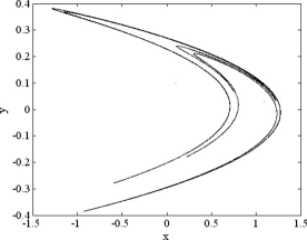
Figure 1: The Strange Attractor of Hénon

3 Pseudorandom Sequence Generation Scheme

Generating a pseudorandom binary sequence from the orbit of a chaotic map essentially requires mapping the state of the system to $\left\{0,1\right\}$. For the Hénon map, consider the two bits $b_{x}$ and $b_{y}$ derived respectively from the $x$ and $y$ state-variables as follows:

$$b_{x} = \left\{\begin{array}[]{rll}1&\mbox{if}&x>\tau_{x}\enspace;\\ 0&\mbox{if}&x\leq\tau_{x}\enspace.\end{array}\right.$$ (5)

$$b_{y} = \left\{\begin{array}[]{rll}1&\mbox{if}&y>\tau_{y}\enspace;\\ 0&\mbox{if}&y\leq\tau_{y}\enspace.\end{array}\right.$$ (8)

Here, $\tau_{x}$ and $\tau_{y}$ are appropriately chosen threshold values for state-variables $x$ and $y$. $\tau_{x}$ should be chosen such that the likelihood of $x>\tau_{x}$ is equal to that of $x\leq\tau_{x}$. The median of a large set of numbers has precisely this property. Therefore, we choose $\tau_{x}$ as the median of a large number $\left(T\right)$ of consecutive values of $x$. Similarly, we assign to $\tau_{y}$, the value of the median of $T$ consecutive values of $y$. Thus, two streams of bits $S_{x}=\left\{b_{x}^{i}\right\}_{i=1}^{\infty}$ and $S_{y}=\left\{b_{y}^{i}\right\}_{i=1}^{\infty}$ are obtained from the map. Consider the bit-stream $B_{x}$ formed by choosing every $P$th bit of $S_{x}$, i.e., $B_{x}=\left\{b_{x}^{Pi}\right\}_{i=1}^{\infty}$. Consider the similarly formed bit-stream $B_{y}=\left\{b_{y}^{Pi}\right\}_{i=1}^{\infty}$. Let us denote the $j$th bit of these two sequences respectively as $B_{x}\left(j\right)$ and $B_{y}\left(j\right)$. Then, the pseudo-random output bit $O$ is chosen as per the following rule:

$$O\left(j\right)=\left\{\begin{array}[]{rll}B_{x}\left(j\right)&\mbox{if}&B_{y}\left(j-2\right)=0\mbox{ and }B_{y}\left(j-1\right)=0\enspace;\\ \overline{B}_{x}\left(j\right)&\mbox{if}&B_{y}\left(j-2\right)=0\mbox{ and }B_{y}\left(j-1\right)=1\enspace;\\ B_{y}\left(j\right)&\mbox{if}&B_{y}\left(j-2\right)=1\mbox{ and }B_{y}\left(j-1\right)=0\enspace;\\ \overline{B}_{y}\left(j\right)&\mbox{if}&B_{y}\left(j-2\right)=1\mbox{ and }B_{y}\left(j-1\right)=1\enspace.\end{array}\right.$$ (9)

Here, $\overline{B}_{x}$ and $\overline{B}_{y}$ respectively denote the logical inverse of $B_{x}$ and $B_{y}$. For $j=0$, $B_{y}\left(-2\right)$ and $B_{y}\left(-1\right)$ can arbitrarily be assumed to be $0$.

The author has found that generated pseudorandom sequences have good statistical properties when $P$ is large. The author has used $P$ between 75 and 5000 depending on the available time for computation and the length of the sequence required. In this paper, sequences generated using this method are called Hénon map sequences.

4 Linear Complexity Properties

A Linear Feedback Shift Register (LFSR) is said to generate an $N$-bit sequence $W$ if for some initial state, the first $N$ bits of the output sequence of the LFSR are the same as $W$ [Golomb 1964, Golomb 1982]. The length of the shortest LFSR that generates $W$ is known as its Linear Complexity.

The author has measured the linear complexity of a large number of even-length Hénon map sequences using the Berlekamp-Massey Algorithm (BMA) [Massey 1969]. The linear complexities obtained for each sequence-length were found to follow a certain probabilistic pattern. In particular, the probability of the linear complexity $C$ of an $N$-bit sequence being equal to $c\left(c<N\right)$, when $N$ is even, was found to be very close to

$$P\left(C=c\right)=\left\{\begin{array}[]{lll}\left(0.5\right)^{N-2c+1}&\quad\mbox{if }&c\leq N/2\enspace;\\ \left(0.5\right)^{2c-N}&\quad\mbox{if }&c>N/2\enspace.\end{array}\right.$$ (10)

To illustrate the correctness of this conjecture, the experimentally determined distribution of linear complexities for 64-bit Hénon map sequences is shown in figure 2 a) alongside the conjectured distribution in figure 2 b) that has been computed using (10). The mean value of linear complexities obtained in this experiment was found to be 32.2083. The expectation of linear complexity for a 64-bit random sequence is 32.2222 and is found to be very close to that of the Hénon map sequences [Menezes et al 1997]. The variance of linear complexities of 64-bit sequences obtained by experiment was 1.0811 against 1.0617 for random sequences.

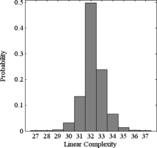
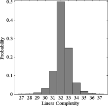
a)  experimental	b)  as per (10)

Figure 2: Probability Distribution of Linear Complexity: 64-bit sequences

Similarly, the probability of the linear complexity $C$ assuming the value $c\left(c<N\right)$ when $N$ is odd was found to be very close to

$$P\left(C=c\right)=\left\{\begin{array}[]{lll}\left(0.5\right)^{N-2c+1}&\quad\mbox{if }&c<\left(N+1\right)/2\enspace;\\ \left(0.5\right)^{2c-N}&\quad\mbox{if }&c\geq\left(N+1\right)/2\enspace.\end{array}\right.$$ (11)

Again, in fig. 3 a), the experimental distribution is shown along with the experimentally determined distribution in fig. 3 b) for 65-bit Hénon map sequences. The experimentally measured mean of linear complexities of these sequences was 32.7663 against the expected 32.7778 for random sequences. Also, the measured variance of linear complexities stands at 1.1177 against 1.0617 for random sequences [Menezes et al 1997].

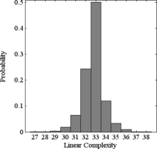
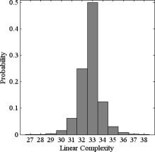
a)  experimental	b)  as per (11)

Figure 3: Probability Distribution of Linear Complexity: 65-bit sequences

Let $W$ be an $N$-bit binary sequence. Let $W_{i}\left(i=1,2,\ldots,N\right)$ denote the subsequence of $W$ consisting of its first $i$ bits. Let $C_{i}$ denote the linear complexity of $W_{i}$. Then the sequence of linear complexities $\left(C_{1},C_{2},C_{3},\ldots,C_{N}\right)$ is known as the linear complexity profile of $W$. For random sequences, the linear complexity profile is expected to be very close to the $C_{i}=i/2$ line (Menezes et al 1997). The linear complexity profile of a sample 553-bit sequence was determined using the Berlekamp-Massey Algorithm. The obtained profile is shown in fig. 4 and can be seen to be very close to the $C_{i}=i/2$ line.

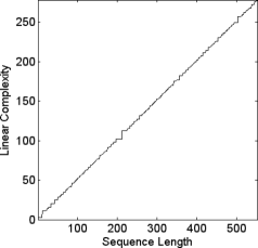
Figure 4: Linear Complexity Profile

5 Correlation Properties

Consider two $N$-bit binary sequences $U$ and $V$. Let $A$ be the number of bit-by-bit agreements between the two. The number of bit-by-bit disagreements must be $D=\left(N-A\right)$. Then the correlation $\theta$ of the two sequences is defined as

$$\theta\left(U,V\right)=\left(A-D\right)/N\enspace.$$ (12)

Theorem 1

If $\;U$ and $V$ are two $N$-bit random binary sequences, the probability of their correlation $\theta$ assuming the value $\Theta$ is given by

$$P\left(\theta=\Theta\right)=\sqrt{\frac{2}{N\pi}}\;e^{-N\Theta^{2}/2}$$ (13)

when

$$\Theta\in\left\{\begin{array}[]{ll}\left\{0,\pm{\frac{2}{N}},\pm{\frac{4}{N}},\ldots,\pm{1}\right\}&\mbox{for even }N,\\ \left\{\pm{\frac{1}{N}},\pm{\frac{3}{N}},\pm{\frac{5}{N}},\ldots,\pm{1}\right\}&\mbox{for odd }N.\end{array}\right.$$

The probability is zero for other values of $\Theta$.

Proof: Since the probability of occurrence of a one is the same as the probability of occurrence of a zero in a truly random sequence, the probability of occurrence of an agreement $\left(p=0.5\right)$ is the same as the probability of occurrence of a disagreement $\left(1-p=0.5\right)$ in a pair of such sequences. Therefore, the number of agreements $A$ in a pair of such sequences is a random variable that follows the binomial distribution with mean $\mu=N/2$ and standard deviation $\sigma=\sqrt{N}/2$. Therefore

$$P\left(A=r\right)=\frac{{}^{N}\!C_{r}}{2^{N}}\enspace.$$ (14)

Applying the Normal approximation to the binomial distribution [Keeping 1962, Ramasubramanian 1997],

$$P\left(A=r\right)\approx\sqrt{\frac{2}{N\pi}}\;e^{-2\left(r-N/2\right)^{2}/N}\enspace.$$ (15)

The correlation $\theta$ is related to the number of agreements $A$ as

$$\theta=\frac{2A}{N}-1.$$ (16)

As $A\in\left\{0,1,2,\ldots,N\right\}$, $\theta\in\left\{-1,\left(\frac{2}{N}-1\right),\left(\frac{4}{N}-1\right),\ldots,1\right\}$. Therefore, $\theta\in\left\{0,\pm{\frac{2}{N}},\pm{\frac{4}{N}},\ldots,\pm{1}\right\}$ for even $N$ and $\theta\in\left\{\pm{\frac{1}{N}},\pm{\frac{3}{N}},\pm{\frac{5}{N}},\ldots,\pm{1}\right\}$ for odd $N$. Clearly, the probability of $\theta$ assuming any other value is zero. By (15) and (16), if $\Theta$ belongs to the above set of valid values,

$$P\left(\theta=\Theta\right)=\sqrt{\frac{2}{N\pi}}\;e^{-N\Theta^{2}/2}$$ (17)

which completes the proof.

The correlation between pairs of Hénon map sequences was experimentally determined and the probability distribution was found to be very close to that of (13). As an illustration, the probability distribution for 127-bit Hénon map sequences and the expected distribution for random sequences are shown in Fig. 5.

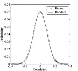
Figure 5: Probability Distribution of Correlation. The legend Random is used for a plot of (13)

The correlation of a sequence with a cyclic-shift of itself is known as its cyclic auto-correlation. Let $W$ be an $N$-bit sequence and $W^{j}$ denote $W$ cyclically right-shifted by $j$ bits. Then the cyclic auto-correlation function of $W$ is defined as $R\left(j\right)=\theta\left(W,W^{j}\right)$. The (cyclic) auto-correlation function of a random sequence is expected to be unity at $j=0$ and close to zero at all other values of $j$. This indeed was found to be the case with Hénon map sequnces. The auto-correlation function of a 2000-bit Hénon map sequence is shown in fig. 6. In the figure, a negative value of shift signifies cyclic left-shifting by an amount equal to the magnitude.

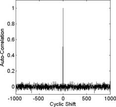
Figure 6: Auto-Correlation Function

6 Statistical Testing

A number of sequences were generated by the algorithm and were subjected to statistical tests. The tests carried out were Menezes et al’s basic tests of randomness [Menezes et al 1997], FIPS 140-1 [FIPS PUB 140-1] recommended battery of tests and National Institute of Standards and Technology (NIST) battery of tests [Rukhin et al 2001].

Menezes et al have proposed a set of five basic tests consisting of frequency test, serial test, poker test, runs test and auto-correlation test. While the first four tests were carried out once for a given sequence, the auto-correlation test was carried out for all possible shifted-versions of the sequence. The result of each test is a test statistic which is compared with a threshold value (one-sided test). The test results in a failure if the threshold is exceeded. The tests were carried out at a significance level of 0.01, hence 1% of failures were expected even for random sequences.

FIPS 140-1 recommends a set of statistical tests for cryptographic random/ pseudorandom number generators. The tests are carried out on a bit-stream of 20,000 bits. The recommended tests are monobit, poker, runs and long-run tests. Each test is a two-sided test where a test-statistic is required to lie within an interval. Though FIPS 140-1 has subsequently been superceded by FIPS 140-2 [FIPS PUB 140-2], since the latter standard does not recommend any statistical tests for cryptographic random/ pseudorandom number generators, the author has used the older recommendations of FIPS 140-1 to evaluate Hénon map sequences.

NIST has forumulated a statistical test suite for random/ pseudo-random number generators to be used for cryptographic applications. The suite consists of a battery of sixteen tests namely 1) Frequency (monobit) test, 2) Frequency test within a block, 3) Runs test, 4) Test for longest run of ones in a block, 5) Binary matrix rank test, 6) Discrete Fourier Transform (spectral) test, 7) Non-overlapping template matching test, 8) Overlapping template matching test, 9) Maurer’s universal statistical test, 10) Lempel-Ziv compression test, 11) Linear complexity test, 12) Serial test, 13) Approximate entropy test, 14) Cumulative sums test, 15) Random excursions test and 16) Random excursions variant test.

7 Statistical Test Results

7.1 Menezes et al’s basic tests of randomness

Two 128-bit sequences $R_{1}$ and $R_{2}$ were generated using parameters shown in table 1. The notation used for test-statistics is the same as those in (Menezes et al 1997). The statistic $X_{5}$ of the auto-correlation test is a function of the value of the relative circular shift. In this case, the value of the relative circular shift is shown in brackets. For example, the statistic obtained by running the auto-correlation test on the sequence and its 3-shifted version is denoted by $X_{5}\left(3\right)$. A similar notation is used for the statistic $X_{3}$ of the poker test where $X_{3}$ depends on the length of the non-overlapping sub-sequences. The results of the tests on the sequences are shown in table 2.

Parameter	$\mathbf{R_{1}}$	$\mathbf{R_{2}}$
$\alpha$	1.40	1.20
$\beta$	0.30	0.30
$x_{0}$	-0.75	-0.75
$y_{0}$	-0.02	0.32
$B_{y}\left(-2\right)$	0	0
$B_{y}\left(-1\right)$	1	1
$P$	24	24
$T$	1000	1000

Table 1: Parameters used for Menezes’ test samples

Statistic	Expected	$\mathbf{R_{1}}$	Result $\mathbf{\left(R_{1}\right)}$	$\mathbf{R_{2}}$	Result $\mathbf{\left(R_{2}\right)}$
$X_{1}$	$<6.634897$	0.125000	Pass	6.125000	Pass
$X_{2}$	$<9.210340$	0.213583	Pass	6.245079	Pass
$X_{3}\left(2\right)$	$<11.344867$	4.625000	Pass	7.625000	Pass
$X_{3}\left(3\right)$	$<18.475307$	1.809524	Pass	9.428571	Pass
$X_{4}$	$<9.210340$	0.890713	Pass	5.373956	Pass
$X_{5}\left(1\right)$	$\left|X_{5}\left(\cdot\right)\right|<2.326348$	0.443678	Pass	-0.088736	Pass
$X_{5}\left(2\right)$	$\left|X_{5}\left(\cdot\right)\right|<2.326348$	0.178174	Pass	1.069045	Pass
$X_{5}\left(3\right)$	$\left|X_{5}\left(\cdot\right)\right|<2.326348$	0.268328	Pass	-0.98387	Pass
$X_{5}\left(4\right)$	$\left|X_{5}\left(\cdot\right)\right|<2.326348$	-1.257237	Pass	-0.179605	Pass
$X_{5}\left(5\right)$	$\left|X_{5}\left(\cdot\right)\right|<2.326348$	-0.631169	Pass	-0.811503	Pass
$X_{5}\left(6\right)$	$\left|X_{5}\left(\cdot\right)\right|<2.326348$	0	Pass	-0.724286	Pass
$X_{5}\left(7\right)$	$\left|X_{5}\left(\cdot\right)\right|<2.326348$	0.272727	Pass	0.272727	Pass
$X_{5}\left(8\right)$	$\left|X_{5}\left(\cdot\right)\right|<2.326348$	-0.730297	Pass	-0.912871	Pass
$X_{5}\left(9\right)$	$\left|X_{5}\left(\cdot\right)\right|<2.326348$	-0.09167	Pass	0.09167	Pass
$X_{5}\left(10\right)$	$\left|X_{5}\left(\cdot\right)\right|<2.326348$	1.288804	Pass	0	Pass
$X_{5}\left(11\right)$	$\left|X_{5}\left(\cdot\right)\right|<2.326348$	0.09245	Pass	-0.64715	Pass
$X_{5}\left(12\right)$	$\left|X_{5}\left(\cdot\right)\right|<2.326348$	0	Pass	0	Pass
$X_{5}\left(13\right)$	$\left|X_{5}\left(\cdot\right)\right|<2.326348$	0.466252	Pass	-0.466252	Pass
$X_{5}\left(14\right)$	$\left|X_{5}\left(\cdot\right)\right|<2.326348$	0.749269	Pass	-0.561951	Pass
$X_{5}\left(15\right)$	$\left|X_{5}\left(\cdot\right)\right|<2.326348$	-0.658505	Pass	-0.282216	Pass
$X_{5}\left(16\right)$	$\left|X_{5}\left(\cdot\right)\right|<2.326348$	0.188982	Pass	-0.377964	Pass
$X_{5}\left(17\right)$	$\left|X_{5}\left(\cdot\right)\right|<2.326348$	1.233905	Pass	-1.993232	Pass
$X_{5}\left(18\right)$	$\left|X_{5}\left(\cdot\right)\right|<2.326348$	0.381385	Pass	-2.097618	Pass
$X_{5}\left(19\right)$	$\left|X_{5}\left(\cdot\right)\right|<2.326348$	-0.287348	Pass	-0.478913	Pass
$X_{5}\left(20\right)$	$\left|X_{5}\left(\cdot\right)\right|<2.326348$	-1.539601	Pass	-0.96225	Pass
$X_{5}\left(21\right)$	$\left|X_{5}\left(\cdot\right)\right|<2.326348$	1.06341	Pass	-0.290021	Pass
$X_{5}\left(22\right)$	$\left|X_{5}\left(\cdot\right)\right|<2.326348$	0.194257	Pass	-1.748315	Pass
$X_{5}\left(23\right)$	$\left|X_{5}\left(\cdot\right)\right|<2.326348$	1.85421	Pass	-2.04939	Pass
$X_{5}\left(24\right)$	$\left|X_{5}\left(\cdot\right)\right|<2.326348$	0.784465	Pass	0.392232	Pass
$X_{5}\left(25\right)$	$\left|X_{5}\left(\cdot\right)\right|<2.326348$	1.280928	Pass	0.68973	Pass
$X_{5}\left(26\right)$	$\left|X_{5}\left(\cdot\right)\right|<2.326348$	1.782266	Pass	-0.594089	Pass
$X_{5}\left(27\right)$	$\left|X_{5}\left(\cdot\right)\right|<2.326348$	-0.298511	Pass	-0.298511	Pass
$X_{5}\left(28\right)$	$\left|X_{5}\left(\cdot\right)\right|<2.326348$	-0.4	Pass	-1.8	Pass
$X_{5}\left(29\right)$	$\left|X_{5}\left(\cdot\right)\right|<2.326348$	1.306549	Pass	1.105542	Pass
$X_{5}\left(30\right)$	$\left|X_{5}\left(\cdot\right)\right|<2.326348$	0.808122	Pass	0.606092	Pass
$X_{5}\left(31\right)$	$\left|X_{5}\left(\cdot\right)\right|<2.326348$	1.929158	Pass	-0.507673	Pass
$X_{5}\left(32\right)$	$\left|X_{5}\left(\cdot\right)\right|<2.326348$	0	Pass	-0.408248	Pass
$X_{5}\left(33\right)$	$\left|X_{5}\left(\cdot\right)\right|<2.326348$	-0.102598	Pass	0.307794	Pass
$X_{5}\left(34\right)$	$\left|X_{5}\left(\cdot\right)\right|<2.326348$	0	Pass	-0.206284	Pass
$X_{5}\left(35\right)$	$\left|X_{5}\left(\cdot\right)\right|<2.326348$	0.933257	Pass	-2.384989	Fail
$X_{5}\left(36\right)$	$\left|X_{5}\left(\cdot\right)\right|<2.326348$	0.625543	Pass	-0.208514	Pass
$X_{5}\left(37\right)$	$\left|X_{5}\left(\cdot\right)\right|<2.326348$	-0.314485	Pass	-0.943456	Pass
$X_{5}\left(38\right)$	$\left|X_{5}\left(\cdot\right)\right|<2.326348$	-0.843274	Pass	-1.897367	Pass
$X_{5}\left(39\right)$	$\left|X_{5}\left(\cdot\right)\right|<2.326348$	-0.317999	Pass	-0.317999	Pass
$X_{5}\left(40\right)$	$\left|X_{5}\left(\cdot\right)\right|<2.326348$	-1.918806	Pass	-0.639602	Pass
$X_{5}\left(41\right)$	$\left|X_{5}\left(\cdot\right)\right|<2.326348$	1.393746	Pass	-0.964901	Pass
$X_{5}\left(42\right)$	$\left|X_{5}\left(\cdot\right)\right|<2.326348$	-0.862662	Pass	0.215666	Pass
$X_{5}\left(43\right)$	$\left|X_{5}\left(\cdot\right)\right|<2.326348$	-0.325396	Pass	-0.325396	Pass
$X_{5}\left(44\right)$	$\left|X_{5}\left(\cdot\right)\right|<2.326348$	-1.309307	Pass	-0.872872	Pass
$X_{5}\left(45\right)$	$\left|X_{5}\left(\cdot\right)\right|<2.326348$	1.426935	Pass	-1.426935	Pass
$X_{5}\left(46\right)$	$\left|X_{5}\left(\cdot\right)\right|<2.326348$	-0.441726	Pass	-0.220863	Pass
$X_{5}\left(47\right)$	$\left|X_{5}\left(\cdot\right)\right|<2.326348$	-1	Pass	0.777778	Pass
$X_{5}\left(48\right)$	$\left|X_{5}\left(\cdot\right)\right|<2.326348$	-0.67082	Pass	-0.447214	Pass
$X_{5}\left(49\right)$	$\left|X_{5}\left(\cdot\right)\right|<2.326348$	-1.237597	Pass	-1.012579	Pass
$X_{5}\left(50\right)$	$\left|X_{5}\left(\cdot\right)\right|<2.326348$	0.452911	Pass	0.679366	Pass
$X_{5}\left(51\right)$	$\left|X_{5}\left(\cdot\right)\right|<2.326348$	-1.025645	Pass	0.797724	Pass
$X_{5}\left(52\right)$	$\left|X_{5}\left(\cdot\right)\right|<2.326348$	-0.458831	Pass	0.458831	Pass
$X_{5}\left(53\right)$	$\left|X_{5}\left(\cdot\right)\right|<2.326348$	-0.11547	Pass	-0.57735	Pass
$X_{5}\left(54\right)$	$\left|X_{5}\left(\cdot\right)\right|<2.326348$	-0.464991	Pass	-1.394972	Pass
$X_{5}\left(55\right)$	$\left|X_{5}\left(\cdot\right)\right|<2.326348$	-0.819288	Pass	-0.117041	Pass
$X_{5}\left(56\right)$	$\left|X_{5}\left(\cdot\right)\right|<2.326348$	0.235702	Pass	-0.471405	Pass
$X_{5}\left(57\right)$	$\left|X_{5}\left(\cdot\right)\right|<2.326348$	-1.780172	Pass	0.593391	Pass
$X_{5}\left(58\right)$	$\left|X_{5}\left(\cdot\right)\right|<2.326348$	-0.717137	Pass	0.239046	Pass
$X_{5}\left(59\right)$	$\left|X_{5}\left(\cdot\right)\right|<2.326348$	-1.324244	Pass	-1.083473	Pass
$X_{5}\left(60\right)$	$\left|X_{5}\left(\cdot\right)\right|<2.326348$	-0.242536	Pass	0.242536	Pass
$X_{5}\left(61\right)$	$\left|X_{5}\left(\cdot\right)\right|<2.326348$	1.588203	Pass	-0.855186	Pass
$X_{5}\left(62\right)$	$\left|X_{5}\left(\cdot\right)\right|<2.326348$	-0.246183	Pass	-1.723281	Pass
$X_{5}\left(63\right)$	$\left|X_{5}\left(\cdot\right)\right|<2.326348$	0.620174	Pass	0.124035	Pass
$X_{5}\left(64\right)$	$\left|X_{5}\left(\cdot\right)\right|<2.326348$	-0.5	Pass	0.5	Pass

Table 2: Testing for Menezes’ Basic Tests of Randomness

7.2 FIPS 140-1

Testing for compliance with FIPS 140-1 is required to be carried out with sequences of 20,000 bits. Five sequences $S_{1}$ through $S_{5}$ were generated using parameters shown in table 3. The results of the tests on the sequences are shown in table 4.

Parameter	$\mathbf{S_{1}}$	$\mathbf{S_{2}}$	$\mathbf{S_{3}}$	$\mathbf{S_{4}}$	$\mathbf{S_{5}}$
$\alpha$	1.23	1.40	1.40	1.40	1.41
$\beta$	0.25	0.25	0.30	0.30	0.21
$x_{0}$	-1.0	-1.0	-1.0	-1.0	-1.0
$y_{0}$	1.0	1.0	1.0	1.0	1.0
$B_{y}\left(-2\right)$	0	0	0	0	0
$B_{y}\left(-1\right)$	1	1	1	1	1
$P$	84	84	84	24	24
$T$	1000	1000	1000	1000	1000

Table 3: Parameters used for FIPS 140-1 test samples

Statistic	Expected	$\mathbf{S_{1}}$	$\mathbf{S_{2}}$	$\mathbf{S_{3}}$	$\mathbf{S_{4}}$	$\mathbf{S_{5}}$
$n_{1}$	$9654<n_{1}<10346$	9938	10107	9944	10099	10020
$X_{3}$	$1.03<X_{3}<57.40$	17.25	13.03	12.98	14.73	6.66
$B_{1}$	$2267<B_{1}<2733$	2572	2473	2560	2480	2454
$G_{1}$	$2267<G_{1}<2733$	2452	2524	2534	2554	2447
$B_{2}$	$1079<B_{2}<1421$	1192	1231	1200	1286	1268
$G_{2}$	$1079<G_{2}<1421$	1302	1264	1226	1262	1310
$B_{3}$	$502<B_{3}<748$	640	643	653	636	616
$G_{3}$	$502<G_{3}<748$	611	577	638	582	580
$B_{4}$	$223<B_{4}<402$	277	319	320	312	312
$G_{4}$	$223<G_{4}<402$	328	315	306	336	314
$B_{5}$	$90<B_{5}<223$	140	165	162	150	156
$G_{5}$	$90<G_{5}<223$	156	165	168	148	159
$B_{6}$	$90<B_{6}<223$	180	159	134	159	164
$G_{6}$	$90<G_{6}<223$	151	146	157	142	159
Result	Pass/Fail	Pass	Pass	Pass	Pass	Pass

Table 4: Testing for FIPS 140-1

7.3 NIST Statistical Test Suite

For each test-run of the test-suite, a sequence of $2\times 10^{8}$ bits was generated and the test-suite was configured to consider this sequence as 200 sequences of $1\times 10^{6}$ bits each. This set of $200$ sequences was subjected to statistical testing in each case. In this manner, the distribution of failures could also be examined by the test-suite and appropriate analysis could be carried out.

The test was carried out on two sets $U_{1}$ and $U_{2}$ of 200-samples each. The parameters used for generating these sets of sequences are shown in table 5.

Parameter	$\mathbf{U_{1}}$	$\mathbf{U_{2}}$
$\alpha$	1.40	1.398
$\beta$	0.30	0.283
$x_{0}$	-1	0.26
$y_{0}$	1	0.29
$B_{y}\left(-2\right)$	0	0
$B_{y}\left(-1\right)$	1	1
$P$	117	111
$T$	1000	1000

Table 5: Parameters used for NIST test samples

For a sample of 200 sequences, the minimum proportion of sequences required to pass all the tests of the suite other than the random excursions (variant) test is 0.968893. The proportion of sequences passing these tests was found to be larger than this threshold. For the random excursions (variant) test, the required minimum passing proportion was found to be 0.961540 and 0.962864 for $U_{1}$ and $U_{2}$ respectively. $U_{1}$ and $U_{2}$ were found to meet this requirement also. The author has noticed, however, that some of the sequences that pass the FIPS 140-1 and Menezes’ tests do not pass the NIST suite of tests. For example, a set of sequences generated using the same parameters as $R_{1}$ was found to fail in the NIST suite. The author has found that passing the NIST suite requires a more careful choice of the parameters. In this case, increasing the value of $T$ to a sufficiently large value resulted in the sequences passing the NIST suite.

8 Keyspace Size

The properties of Hénon map sequences presented in the preceding sections demonstrate that they are potential candidates for cryptographic applications. A Hénon map sequence can be used, for example, can be directly Exclusive-ORed, bit-by-bit, with a data sequence of the same length. Such a cipher is popularly known as the Vernam Cipher [Kippenhahn 1999, Mollin 2001]. The values of $\alpha,\beta,x_{0},y_{0}$ and the sampling-factor $P$ together can form the key. In this section, an attempt is made to estimate the size of the keyspace for such a cipher.

The author has found that $\alpha$ in $\left(1.16,1.41\right)$ and $\beta$ in $\left(0.2,0.3\right)$ are useful for generating sequences with the desired statistical properties. Also, we can assume $x_{0}$ to lie in $\left(-1,1\right)$ and $y_{0}$ to lie in $\left(-0.35,0.35\right)$. $P$ can be assumed within $\left(80,1000\right)$. Though these limits are in no way binding or accurate, they should give a reasonable estimate of the size of the keyspace. The size of the keyspace then depends on the precision of the computing platform on which the cipher algorithm is implemented. With 32-bit floating-point numbers of the IEEE format, the smallest possible increment $\left(\epsilon\right)$ is $\epsilon_{32}\approx 1.1921\times 10^{-7}$. With 64-bit floating-point numbers this value is $\epsilon_{64}\approx 2.2204\times 10^{-16}$. Let $\hat{\alpha}$ indicate the size of the interval over which $\alpha$ can span i.e. $\hat{\alpha}=1.41-1.16$. Let $\hat{\beta},\hat{x_{0}},\hat{y_{0}}$ and $\hat{P}$ have correspondingly similar meaning. Since $P$ is an integer, $\hat{P}=1000-80$. Then, the number of representable values of $\alpha$ on the applicable computing platform can be computed as $K_{\alpha}=\hat{\alpha}/\epsilon$. Such a calculation can easily be carried out using logarithms. Similarly, $K_{\beta},K_{x_{0}}$ and $K_{y_{0}}$ can also be calculated. $K_{P}=\hat{P}$. Since the parameters are used together, the size of the keyspace $K=K_{\alpha}\times K_{\beta}\times K_{x_{0}}\times K_{y_{0}}\times K_{P}$. The logarithm of this figure, to the base 2, gives an estimate of the length of a single binary key which contains all the information required to generate the pseudo-random sequence. The value of $\log_{2}\left(K\right)$ for 32-bit and 64-bit precision was found to be 97 and 213 respectively. The size of the keyspace can be further increased by increasing the precision of floating-point representation.

9 Concluding Remarks

Though chaotic orbits of discrete-time maps are non-periodic in nature, because of finite precision of digital computers the orbits actually turn out to be periodic. The average period of an orbit of a two-dimensional map can be expected to be longer than that of a one-dimensional map. To overcome the inevitable periodicity in digital computation, Shujun et al have used simple LFSR-based perturbation generators to perturb the parameters of the dynamical systems used [Shujun et al 2001]. Though they have used perturbed one-dimensional maps in couple-chaotic-system-based pseudorandom sequence generators, the same technique should be directly applicable to the present algorithm and is a feasible way of defeating the periodicity.

The periodicity inherent in digital-computer implementations is not a problem in maps realized on an analog-computer. The Hénon map, due to its polynomial form, can be realized in the form of an electronic circuit using analog-multipliers, sample-and-hold blocks and operational amplifiers. Such a realization of the logistic map has already been studied [Suneel 2006]. The advantage of an analog realization of chaotic maps is that due to natural variations in circuit parameters and conditions, practically identical systems provided with practically identical conditions generate sequences that quickly diverge and become un-correlated within a short time. Therefore, such implementations may actually turn out to be truly random (as opposed to pseudorandom) sequence generators.

The choice of the Hénon map for the work in this paper was rather arbitrary. The author believes that similar results should also be attainable with other two-dimensional maps.

The linear complexity and correlation properties of the proposed sequences suggest a strong similarity to random sequences. Results of statistical tests carried out confirm this further. A large size of the keyspace suggests strong candidature for cryptographic applications, especially for stream cipher cryptography. Possible cryptanalysis techniques for these sequences is an open subject.

10 Acknowledgements

The author thanks his colleagues A.P. Dabhade, K.V. Suresh, D. Venu Gopal and R.S. Chandrasekhar for several hours of discussions.

References

- [Crutchfield et al 1986] Crutchfield J P, Farmer J D, Packard N H, Shaw R S 1986 Chaos, Sci. Amer. 255:38-49
- [Dachselt & Schwarz 2001] Dachselt F, Schwarz W 2001 Chaos and Cryptography, IEEE Trans. Circ. Sys. - I 48:1498-1509
- [Falcioni et al 2006] Falcioni M, Palatella L, Pigolotti S, Vulpiani A 2006 Properties Making a Chaotic System a Good Pseudo Random Number Generator, ePrint arXiv:nlin.CD/0503035
- [FIPS PUB 140-1] FIPS PUB 140-1, Federal Information Processing Standards Publication - Security Requirements for Cryptographic Modules, U.S. Department of Commerce, 11 January 1994
- [FIPS PUB 140-2] FIPS PUB 140-2, Federal Information Processing Standards Publication - Security Requirements for Cryptographic Modules, U.S. Department of Commerce, 25 May 2001
- [Gleick 1997] Gleick J 1997 Chaos, (London: Vintage)
- [Golomb 1964] Golomb S W 1964 Introduction to Digital Communication in Golomb S W [ed] Digital Communications with Space Applications, (Englewood Cliffs: Prentice Hall) pp 1-16
- [Golomb 1982] Golomb S W 1982 Shift Register Sequences, (Laguna Hills: Aegean Park Press) pp 1-108
- [Hénon 1976] Hénon M 1976 A Two-dimensional Mapping with a Strange Attractor, Commun. Math. Phys. 50:69 77
- [Alligood et al 1997] Alligood K T, Sauer T D, Yorke J A 1997 Chaos - An Introduction to Dynamical Systems (New York: Springer-Verlag) pp 43-91, 163-166, 238-239
- [Keeping 1962] Keeping E S 1962 Introduction to Statistical Inference (Princeton: D. Van ostrand) pp 64-66
- [Kippenhahn 1999] Kippenhahn R 1999 Code Breaking: A History and Exploration (Hyderabad: Universities Press) pp 201-204
- [Knuth 1998] Knuth D E 1998 The Art of Computer Programming, Volume 2/Seminumerical Algorithms, 3rd ed (Reading: Addison Wesley) pp 9-37
- [Kocarev 2001] Kocarev L 2001 Chaos-Based Cryptography: A Brief Overview, IEEE Circ. & Sys. Mag., 1:6-21
- [Kumar 1996] Kumar N 1996 Deterministic Chaos: Complex Chance out of Simple Necessity, (Hyderabad: Universities Press)
- [Massey 1969] Massey J L 1969 Shift Register Synthesis and BCH Decoding, IEEE Trans. Inform. Theory 15:122-127
- [Menezes et al 1997] Menezes A J, van Oorschot P C, Vanstone S A 1997 Handbook of Applied Cryptography (Boca Raton: CRC Press) pp 198-200
- [Mollin 2001] Mollin R A 2001 An Introduction to Cryptography, (Boca Raton: Chapman and Hall/CRC), pp 115-116
- [Peitgen et al 2004] Peitgen H O, Jürgens H, Saupe D 2004 Chaos and Fractals, New Frontiers of Science, 2nd ed (New York: Springer-Verlag) pp 609-627
- [Ramasubramanian 1997] Ramasubramanian S 1997 The Normal Distribution: From Binomial to Normal, Resonance 2:15-24
- [Rukhin et al 2001] Rukhin A et al 2001 NIST Special Publication 800-22: A Statistical Test Suite for Random and Pseudorandom Number Generators for Cryptographic Applications, National Institute of Standards and Technology.
- [Shujun et al 2001] Shujun L, Xuanqin M, Yuanlong C 2001 Pseudorandom Bit Generator Based on Couple Chaotic Systems and its Applications in Stream Cipher Cryptography, Progress in Cryptology: INDOCRYPT-2001 The 2nd International Conference on Cryptology in India, Indian Institute of Technology, Madras, Chennai, India, 16-20 December 2001.
- [Suneel 2006] Suneel M 2006 Electronic Circuit Realization of the Logistic Map, Sādhanā, 31(1):69-78
- [Woodcock & Smart 1998] Woodcock C F, Smart N P 1998 -adic Chaos and Random Number Generation, Experimental Math., 7:333-342.