On Conditional Branches in Optimal Search Trees

Abstract

Algorithms for efficiently finding optimal alphabetic decision trees — such as the Hu-Tucker algorithm — are well established and commonly used. However, such algorithms generally assume that the cost per decision is uniform and thus independent of the outcome of the decision. The few algorithms without this assumption instead use one cost if the decision outcome is “less than” and another cost otherwise. In practice, neither assumption is accurate for software optimized for today’s microprocessors, which generally have one cost for the more likely decision outcome and a greater cost — often far greater — for the less likely decision outcome. This problem and generalizations thereof are thus applicable to hard coding static decision tree instances in software, e.g., for optimizing program bottlenecks or for compiling switch statements. An $O(n^{3})$-time $O(n^{2})$-space dynamic programming algorithm can solve this optimal binary decision tree problem, and this approach has many generalizations that optimize for the behavior of processors with predictive branch capabilities, both static and dynamic. Solutions to this formulation are often faster in practice than “optimal” decision trees as formulated in the literature. Different search paradigms can sometimes yield even better performance.

I Introduction

Consider a problem of assigning grades to tests. These tests might be administered to humans or to objects, but in either case there are grades $1$ through $n$ — $n$ being $5$ in most academic systems — and the corresponding probabilities of each grade, $p(1)$ through $p(n)$, can be assumed to be known. (If unknown, they are assumed to be identical.) Each grade is determined by taking the actual score, $a$, dividing it by the maximum possible score, $b$, and seeing which of $n$ distinct fixed intervals of the form $[v_{i-1},v_{i})$ the ratio lies in, where $v_{0}=-\infty$ and $v_{n}=+\infty$. This process is repeated for independently determined grades enough times that it is worthwhile to consider the fastest manner in which to determine these scores.

A straightforward manner of assigning scores would be to multiply (or shift) $a$ by a constant $k$ ($\log_{2}k$), divide this by $b$, and use lookup tables on the scaled ratio. However, division is a slow step in most CPUs — and not even a native operation in others — and a lookup table, if large, can take up valuable cache space. The latter problem can be solved by using a numerical comparisons to determine the score, resulting in a decision tree. In fact, with this decision tree, we can eliminate division altogether; instead of comparing scaled ratio $ka/b$ with grade cutoff value, $v_{i}$, we can equivalently compare $ka$ with $bv_{i}$, replacing the slow division of variable integers with a fast multiplication of a variable and a fixed integer. The only matter that remains is determining the structure of the decision tree.

The desired tree has a large variety of applications — e.g., the compilation of switch (case) statements[34, 13] — and such a decision tree is known as an optimal alphabetic binary tree. Algorithms used for finding such trees, however, find trees with minimum expected path length, or, equivalently, minimum expected number of comparisons[27, 19, 9], whereas we want a tree that results in minimum average run time. The general assumption in finding an optimal search tree is that these goals are identical, that is, that each search step (edge) takes the same amount of time (cost) as any other; this is noted in Section 6.2.2 of Knuth’s The Art of Computer Programming[30, p. 429]. In exercise 33 of Section 6.2.2, however, it is conceded that this is not strictly true; in the first edition, the exercise asks for an algorithm for where there is an inequity in cost between a fixed cost for a left branch and a fixed cost for a right branch[28], and, in the second edition, a reference is given to such an algorithm[25]. Such an approach has been extended to cases where each node has a possibly different, but still fixed, asymmetry[35].

In practice the asymmetry of branches in a microprocessor is different in character from any of the aforementioned formulations. On complex CPUs, such those in the Pentium family, branches are predicted as taken or untaken ahead of execution. If the branch is predicted correctly, operation continues smoothly and the branch itself takes only the equivalent of one or two other instructions, as instructions that would have been delayed by waiting for the branch outcome are instead speculatively executed. However, if the branch is improperly predicted, a penalty for misprediction is incurred, as the results of speculatively executed instructions must be discarded and the processor returned to the state it was at prior to the branch[14]. In the case of the Pentium 4 processor, a mispredicted branch takes the equivalent of dozens of instructions[8]. This penalty has only increased with the deeper pipelines of more recent processors. While this time penalty pales in comparison to that taken by division — over a hundred adds and shifts can take place in the time it takes to do one 32-bit division on the Pentium family processors — it certainly reveals comparison tally as being a poor approximation to run time, the ideal minimization.

In this paper, we discuss the construction of alphabetic binary trees — and more general search trees — that are optimized with respect to the behavior of conditional branches in microprocessors. We establish a general dynamic programming paradigm, one applicable to such architecture families as: the Intel Pentium architectures, which use advanced dynamic branch prediction; the ARM architectures, most instances of which use static branch prediction; and Knuth’s MMIX architecture, in which branches explicitly “hint” whether or not they are assumed taken or untaken[31, p. 20]. The first two are not only representative of two styles of branching; they are also by far the most popular processors for 32-bit personal computers and 32-bit embedded applications, respectively. Dynamic programming algorithms with $O(n^{3})$-time $O(n^{2})$-space performance are developed and discussed. Although these algorithms are not simplified in the same manner as Knuth’s dynamic programming algorithm[27], they are fairly flexible, accounting for different costs (run times) for different comparisons due to such behaviors as dynamic branch prediction and conditional instructions other than branches.

II No prediction and static prediction

Consider Knuth’s pedagogical MMIX architecture[31], which has a simple rule for branching: If we know ahead of time which branch is more likely and which less likely, we can hard code the more likely branch to take $1+c$ clock cycles and the less likely branch to take $3+c$ clock cycles, where $c$ represents the time taken by instructions other than the branch itself, e.g., multiplications, additions, comparisons. Note that the disparity in performance between correctly anticipated branches and incorrectly anticipated branches is not as great as that for recent versions of the Pentium architectures, in which the exact number depends on the processor architecture and the type of comparison. For this ubiquitous family of processors, properly modeling the asymmetry of search tree performance is even more vital than it is on MMIX. However, since the MMIX architecture uses hints with no branch prediction, it is simpler to model and to hard code any desired preference. (Some real-world processors such as the Intel Pentium 4[23, p. 2-2] and the MIPS R4000[12, p. 21] also use such branch hints, usually in conjunction with more advanced prediction techniques discussed in the next section.)

It is also easy to code the asymmetric bias of the branch for most implementations of static branch prediction. In static prediction, opcode or branch direction is used to determine whether or not a branch is taken, the most common rule being that forward conditional branches are presumed taken and backward conditional branches are presumed not taken[14]. Assume, for example, that we want to use a forward branch, which is assumed not to be taken. We thus want the most likely outcome to be that the branch is not taken: For example, if it is more likely than not that the item is less than $v_{i}$, the branch instruction should correspond to “branch if greater than or equal to $v_{i}$.” Otherwise, the branch instruction should correspond to “branch if less than $v_{i}$.”

The decision tree problem, applicable to problems with either no branch prediction or static branch prediction, considers positive weights $c_{1}$ and $c_{2}$ such that the cost of a binary path with predictability $b_{1}b_{2}\cdots b_{k}$ is

$$t(b_{1}b_{2}\cdots b_{k})\triangleq\sum_{j=1}^{k}c_{b_{j}}$$

where $b_{j}=1$ for a mispredicted result and $b_{j}=2$ for a properly predicted result. Such tree paths are often pictorially illustrated via longer edges on the corresponding tree, so that path height corresponds to path cost, e.g., Fig. 1(b). Thus the overall expected cost (time) to minimize is

$$T(b)\triangleq\sum_{i=1}^{n}p(i)\sum_{j=1}^{l(i)}c_{b_{j}(i)}$$ (1)

where $p(i)$ is the probability of the $i$th item, $l(i)$ is the number of comparisons needed, and $b_{j}(i)$ is $1$ if the result of the $j$th branch for item $i$ is contrary to the prediction and $2$ otherwise.

Note that if the number of comparisons is the value to be emphasized in pictorial representation, edges can be portrayed with fixed height, as in Fig. 1(a). In Fig. 1(b), by contrast, the total cost is the value emphasized; having edges portrayed in this way, with height proportional to their cost, is usually preferred.

This problem can be placed in the context of optimal binary tree problems, as in Table I. Other than the branching problem considered in this paper, problems are referred to as in [1]. In most problem formulations, edge cost is fixed, and, where it is not fixed, edges generally have costs according to their order, i.e., a left edge has cost $c_{1}$ and a right edge has cost $c_{2}$. Relaxing this edge order constraint in the unequal cost alphabetic problem results in the problem we are now considering. Note that Karp’s nonalphabetic variant does not change if edge order is allowed to change; since output items need not be in a given (e.g., alphabetical) order, the tree optimal for the ordered-edge nonalphabetic problem is also optimal for the unordered-edge nonalphabetic problem. Because of all this, the cost for the optimal tree under Karp’s formulation is a lower bound on the cost of the optimal branch tree, whereas the cost for the optimal tree under Itai’s formulation is an upper bound on the cost of the optimal branch tree. This enables the use of the bounds formulated in [2] for the branching problem.

	Edge cost/order specification
Output order restriction	Constant cost	Order restricted	Order unrestricted
Alphabetic	Hu-Tucker[10, 19, 9, 30]	Itai[25, 35]	branching problem
Nonalphabetic	Huffman[22, 38, 29]	Karp[26, 11, 6]

TABLE I: Types of decision tree problems

The key to constructing an algorithm is to note that any optimal alphabetic tree must have all its subtrees optimal; otherwise one could substitute an optimal subtree for a suboptimal subtree, resulting in a strict improvement in the result. Each tree can be defined by its splitting points. A splitting point $s$ for the root of the tree means that all items after $s$ and including $s$ will be in the right subtree while all items before $s$ will be in the left subtree. Since there are $n-1$ possible splitting points for the root, if we know all potential optimal subtrees for all possible ranges, the splitting point can be found through sequential search of the possible combinations. The optimal tree is thus found inductively, and this algorithm has $O(n^{3})$ time complexity and $O(n^{2})$ space complexity, in a similar manner to [10].

The dynamic programming algorithm, given the aforementioned considerations, is relatively straightforward. Each possible optimal subtree for items $i$ through $j$ has an associated cost, $c(i,j)$ and an associated probability $p(i,j)$; at the end, $p(1,n)=1$ and $c(1,n)$ is the expected cost (run time) of the optimal tree.

The base case and recurrence relation we use are similar to those of [25]. Given unequal branch costs $c_{1}$ and $c_{2}$ and probability mass function $p(\cdot)$ for $1$ through $n$,

$$\begin{array}[]{rcl}c(i,i)&=&0\\ c^{\prime}(i,j)&=&\min_{s\in(i,j]}\{c_{1}p(i,s-1)+c_{2}p(s,j)+{}\\ &&\quad c(i,s-1)+c(s,j)\}\\ c^{\prime\prime}(i,j)&=&\min_{s\in(i,j]}\{c_{2}p(i,s-1)+c_{1}p(s,j)+{}\\ &&\quad c(i,s-1)+c(s,j)\}\\ c(i,j)&=&\min\left\{c^{\prime}(i,j),c^{\prime\prime}(i,j)\right\}\end{array}$$ (2)

where $p(i,j)=\sum_{k=i}^{j}p(i)$ can be calculated on the fly along with $c(i,j)$. The last minimization determines which branch condition to use (e.g., $<$ vs. $\geq$ or “assume taken” vs. “assume untaken”), while the minimizing value of $s$ is the splitting point for that subtree. The branch condition to use — i.e., the bias of the branch — must be coded explicitly or implicitly in the software derived from the tree.

Knuth[27] and Itai[25] also begin with such an algorithm, then go on to note that the splitting point of an optimal tree for their problems must be between the splitting points of the two (possible) optimal subtrees of size $n^{\prime}-1$, and use this fact to reduce complexity. The branching problem considered here, however, lacks this property. Consider $p=(0.3~{}0.2~{}0.2~{}0.3)$ and $c=(3~{}1)$, for which optimal trees split either at $2$, as in Fig. 1, or at $4$, the mirror image of this tree. In contrast, the two largest subtress, as illustrated in the figure and its mirror image, both have optimal split points at $3$. Similarly, applying the less complex Hu-Tucker approach[19, 17] to this problem fails for $p=(0.2~{}0.15~{}0.15~{}0.2~{}0.3)$ and $c=(3~{}1)$.

\psfrag{1}{$1$}\psfrag{3}{$3$}\includegraphics{fixedtree.eps}

(a) Fixed-length representation

\psfrag{1}{$1$}\psfrag{3}{$3$}\includegraphics{proptree.eps}

(b) Proportional representation

Figure 1: Two representations of optimal branch trees

The optimal tree of Fig. 1 is identical to the optimal tree returned by Itai’s algorithm for order-restricted edges[25]. Consider a larger example in which this is not so, the binomial distribution $p=(1\ 6\ 15\ 20\ 15\ 6\ 1)/128$ with $c=(11~{}2)$. If edge order is restricted as in [25], the tree at Fig. 2(a) is optimal, yielding an expected cost of $967/64=15.109375$. If we relax the restriction, as in the problem under consideration here, the tree at Fig. 2(b) is optimal, yielding an expected cost of $831/64=12.984375$, a $14\%$ improvement.

(a) Edge order restricted

(b) Edge order unrestricted

Figure 2: Optimal branch trees for two restriction types for $p=(1\ 6\ 15\ 20\ 15\ 6\ 1)/128$ with $c=(11~{}2)$

The $O(n^{3})$ complexity used to get this better result is generally not limiting. Although this restricts the range of problems solvable within a given time, most hard-coded search tree problems are small enough to be solved quickly. In addition, this model is not robust enough to model performance for large seach trees, where some problems, such as the aforementioned grade-assignment problem, are actually better solved via alternative means when $n$ is large; a division and lookup table might be more suitable, for example, if there are dozens of different grades. This is not only due to the fact that search run time scales as $O(\log n)$, but also because large blocks of software code generally run more slowly due to insufficient instruction caching. If larger problems did need to be solved within this framework, space complexity would likely become an issue before time complexity anyway.

Given no information on $p(\cdot)$, it is common to assume that $p(i)=1/n$. This is justified by noting that, if $p(\cdot)$ is considered a random vector drawn from the probability simplex according to density $g$ — as in [7] — the expected cost for a given coding scheme is

$$E_{p}[T(b)]=E_{p}\left[\sum_{i=1}^{n}p(i)\sum_{j=1}^{l(i)}c_{b_{j}(i)}\right]=\sum_{i=1}^{n}E_{p}[p(i)]\sum_{j=1}^{l(i)}c_{b_{j}(i)}$$

and, if $g$ is symmetric on the simplex, $E[p(i)]=1/n$ for any $i$. Since edge costs are not fixed, optimal trees for this uniform distribution need not be complete trees, that is, full trees for which all leaves have depth $\lfloor\log_{2}n\rfloor$ or $\lceil\log_{2}n\rceil$. For example, the tree in Fig. 1 is optimal for this uniform distribution with an average cost of $3.75$, whereas the complete tree for $n=4$ results in an average cost of $4$. This is thus a better approach to use for compilers that code switch (case) statements partially[13] or entirely[34] as decision trees.

ARM architectures such as those of the ARM7 and ARM9 families use no or static branch prediction[5]. Such processors are used for most mobile devices, including cell phones and iPods. Recent Pentium designs and the XScale[24] — which is viewed as the successor to ARM architecture StrongARM — use dynamic prediction, which we explore in the next section.

III More advanced models

With dynamic branch prediction, which in more advanced forms includes branch correlation, branches are predicted based on the results of prior instances of the same and different branch instructions. This results in improved branch predictability for most software implementations, especially those in which branch profiling does not enter into software design. Where branch profiling does take place, however, the gains are often only marginal[14, pp. 245–248]. Thus, although large processors and general purpose processors generally include dynamic prediction, many small processors and low-power processors forgo dynamic prediction, as this feature’s sophistication requires the usage of significant additional semiconductor area for the associated logic.

Dynamic branch prediction often results in complex processor behavior. Often several predictors will be used for the same branch instruction instance; the predictor in a given iteration will be based on the history of that branch instruction instance and/or other branches. In the problem we are concerned with, however, this does not result in as many complications as one might expect; the probability of a given branch outcome conditional on the branches that precede it is identical to the probability of the branch outcome overall. In the case of previous branch outcomes for the same search instance — i.e., those of ancestors in the tree — any given outcome is conditioned on the same events — i.e., the events that lead to the branch being considered. In the case of branches for previous items, if items are independent, so are these branches. In the case of branches outside of the algorithm, these can also be assumed to be either fixed given or independent of the current branch.

Thus, as long as each branch predictor is assigned at most one of the decision tree branches, prediction can be modeled as a random process. This process will result in each predictor converging to a stationary distribution, which can be analyzed and optimized for. Unfortunately, such a random process will necessarily perform worse than optimized static prediction, although, in most instances, the difference will not be too great.

The cost of each branch result can be determined by the expected time of the branch, based on the costs involved and the probability that the branch is correctly predicted. Simple analysis of the stationary distribution of a branch prediction Markov chain, e.g., [16], can yield the expected time for a given branch direction as a function of the probability of the branch.

For example, if branch prediction uses a saturating up-down counter — the two-bit Markov chain of [33] shown as a Moore state diagram in Fig. 3(a) — then the probability of misprediction is given by

$$f_{{\mathop{\rm A2}}}(p_{1})\triangleq P[\mbox{mispredict on A2}]=\frac{p_{1}-p_{1}^{2}}{1-2p_{1}+2p_{1}^{2}}$$

where $p_{1}$ is the probability the less likely event will occur given the branch being considered. This Markov chain is used by the more recent Pentium architectures[8] and is referred to by Yeh and Patt as Automation A2[39]. If branch prediction instead uses the two-bit Markov chain of [32], as in the MIPS-influenced pedagogical architecture in [14] and in Fig. 3(b), then the probability of a misprediction is given by

$$f_{{\mathop{\rm A3}}}(p_{1})\triangleq P[\mbox{mispredict on A3}]=\frac{p_{1}+p_{1}^{2}+4p_{1}^{3}+2p_{1}^{4}}{1-p_{1}+p_{1}^{2}}.$$

This chain is referred to by Yeh and Patt as Automation A3. (Other state diagrams considered by Yeh and Patt are not in as wide use, either being too simple or lacking symmetry between taken and untaken branches.)

\psfrag{N}{{\small N}}\psfrag{T}{{\small T}}\psfrag{0/N}{{$0$/N}}\psfrag{1/N}{{$1$/N}}\psfrag{2/T}{{$2$/T}}\psfrag{3/T}{{$3$/T}}\includegraphics{A2.eps}

(a) A2 (recent Pentium architectures)

\psfrag{N}{{\small N}}\psfrag{T}{{\small T}}\psfrag{0/N}{{$0$/N}}\psfrag{1/N}{{$1$/N}}\psfrag{2/T}{{$2$/T}}\psfrag{3/T}{{$3$/T}}\includegraphics{A3.eps}

(b) A3 (Computer Architecture – A Quantitative Approach)

Figure 3: Moore state diagrams for branch prediction

The Moore state diagrams for Automations A2 and A3 in Fig. 3 have N representing an untaken branch and T representing a taken branch. The state determines which prediction is made, and the actual branch outcome determines the transitions between the states. The corresponding stationary misprediction rate (Fig. 4) is worst for Automation A3 (dotted plot), which has a rate up to 26.92% worse than that for static prediction (solid plot). Automatic A2 (dashed plot) does better, being at most 20.71% worse than static prediction.

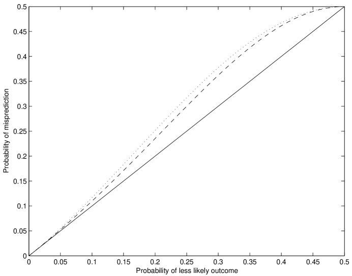
Figure 4: Static and dynamic branch misprediction rates

In either dynamic case, we can calculate expected cost from the probabilities of each branch. We initially assume that taken and untaken branches are symmetric, that is, a branch rightly predicted as untaken will have the same cost as a branch rightly predicted as taken, and mispredicted branches will similarly have identical costs. Let the type of dynamic prediction be $A$, let the probability of the more likely subtree be $p_{\max}$, and let the probability of the less likely subtree be $p_{\min}$, so that $p_{\min}+p_{\max}\leq 1$ and $p_{1}=p_{\min}/(p_{\min}+p_{\max})$ is the probability of the less likely outcome conditional on the branch being decided upon. Then, instead of the static cost of $c_{1}p_{\min}+c_{2}p_{\max}$, the expected cost of a given branch is

$$\begin{array}[]{l}C(p_{\min},p_{\max})\triangleq\\[4.0pt] \quad c_{1}(p_{\min}+p_{\max})f_{A}\left(\frac{p_{\min}}{p_{\min}+p_{\max}}\right)+{}\\[6.0pt] \qquad c_{2}(p_{\min}+p_{\max})\left(1-f_{A}\left(\frac{p_{\min}}{p_{\min}+p_{\max}}\right)\right).\end{array}$$

Thus this plus the costs of the subtrees is the overall tree cost.

Asymmetries in taken and untaken branches are easily accounted for. Similarly, if a $(<,\geq)$ comparison with a certain value has a smaller cost than a comparison with another value — say a comparison with a power of two times a variable is faster due to the inherently reduced calculation time — then this can also be taken into account. Another variant can be found by noting that some processors allow conditional instructions, that is, instructions only executed given certain conditions. On platforms such as those in the Pentium family, a conditional instruction is often preferable to a conditional branch, but this might only reasonably be used to eliminate a branch to leaves in the decision tree. Thus branches deciding between only two items might be accounted differently.

With such a variety of options, there could be multiple possible costs for any particular branch. General cost functions for a branch taking all this into account are of the form $C_{k}(p^{\prime},p^{\prime\prime},i,j,s)$ for $k$ from $1$ to some $m$ (where $m=2$ is most common), and (2) thus becomes:

$$\begin{array}[]{rcl}\displaystyle c(i,i)&=&0\\[4.0pt] c_{k}(i,j)&=&\displaystyle\min_{s\in(i,j]}\{C_{k}(p(i,s-1),p(s,j),i,j,s)+{}\\ &&\quad c(i,s-1)+c(s,j)\}\quad\forall k\\[4.0pt] c(i,j)&=&\displaystyle\min_{k\in[1,m]}\left\{c_{k}(i,j)\right\}\end{array}$$ (3)

Once again, this is a simple matter of dynamic programming, and, assuming all $C_{k}$ are calculable in constant time, this can be done in $O(mn^{3})$ time and $O(n^{2}+n\log m)$ space, the $\log m$ term accounting for recalculation and storage of the type of cost function (decision method) used for each branch. An even more general version of this could take into account properties of subtrees other than those already mentioned, but we need not consider this here.

Note that, because dynamic prediction is adaptive to dynamic branch performance, we need not explicitly code branch bias; the more and less likely branch outcomes will automatically be detected. However, most dynamic predictors begin with state that depends on the type of branch in the same manner as static prediction. That is, the first time a branch is encountered, it is usually statically predicted. Thus it might also be worthwhile to implement the search software so that initial iterations of the search tree behave as well as possible given the tree optimal for asymptotic behavior. Note that this variation adds no time or space complexity to the above algorithm.

If the software is predetermined but the tree is not — that is, if the software is not hard coded for the specific tree — then matters change entirely; no prediction and static prediction result in this problem being equivalent to that of ordered edges, the problem proposed by Knuth and considered by Itai. Dynamic prediction with correlations, on the other hand, can result in a number of outcomes, depending on implementation. The software on a given processor could have near-perfect distinguishing of outcomes, in which the above dynamic analysis persists. More likely, without sufficient unrolling[14] of the tree data structure, there would be confusion of outcomes, as the software would not know whether all previous branches untaken indicates we are at the root, at its right child, at its right child’s right child, etc. Optimizing for the complex dependencies involved with such a system is no longer within the above framework, and the overall averaging effect means that one might want to just use the tree optimal for the corresponding static problem Therefore the aforementioned methods are usually best suited for when the user has the option of designing software specifically for a given decision tree, or designing hardware and/or programmable logic to allow the methods to work in fixed software.

IV Search trees and equality comparisons

Knuth showed how a dynamic programming approach can be used for general search trees[27], in which the decision is no longer binary, but is instead, “Is the output greater than, less than, or equal to $x$?” This allows items to be implicitly or explicitly stored within the internal nodes (nonleaves) of the decision tree and allows us to consider items that might not be in a search tree. This model generalizes the concept of an alphabetic decision tree and can be used for applications in which there is an inherent “dictionary” of items, such as token parsing and spell checking. Probabilities for both present and missing items are then needed.

Before formalizing this, we should note a few things about the applicability of the search tree model. Clearly the problem at the beginning of this paper does not fall into this model, as strict equality cannot be tested for. Even where this model is applicable, it can be too restrictive. For example, this model is often inferior to the alphabetic model for the simple reason that, on most hardware, including all hardware considered here, three-way branches are not native operations. They must thus be simulated by two two-way branches in a manner that actually results in greater run time. Experimental analysis of this phenomenon can be found in [4] and numerical analysis can be found in [20] and [18, pp. 344–345]. These all find that an alphabetic tree is usually preferable in practice. Thus we only briefly discuss issues of this search tree model.

For items $1$ through $n^{\prime}$, $\beta_{i}$ is defined as the probability that a search yields item $i$ and $\alpha_{i}$ as the probability that a search fails and the item not in the search tree would be lexicographically between items $i$ and $i+1$; $\alpha_{0}$ is the probability it is before $\beta_{1}$ and $\alpha_{n}$ is the probability it is after $\beta_{n}$. Thus

$$\sum_{i=1}^{n^{\prime}}\beta_{i}+\sum_{i=0}^{n^{\prime}}\alpha_{i}=1.$$

The alphabetic tree scenario is a special case, with $n^{\prime}=n-1$, $\beta_{i}=0$, and $\alpha_{i}=p(i+1)$, as in Fig. 5(a) for $n=5$. Fig. 5(b) is a similar search tree configured for a three-way comparison; this time, there are only four items, and it is assumed that all items searched for will be in the tree. Fig. 5(c) is the same four-item search tree allowing one to search for both items in the tree (with probabilities $\{\beta_{i}\}$) and ranges of missing items (with probabilities $\{\alpha_{i}\}$).

\psfrag{a0}{$p(1)$}\psfrag{a1}{$p(2)$}\psfrag{a2}{$p(3)$}\psfrag{a3}{$p(4)$}\psfrag{a4}{$p(5)$}\includegraphics{searchalpha.eps}

(a) Alphabetic tree (${\beta}_{i}=0$)

\psfrag{b1}{$p(1)$}\psfrag{b2}{$p(2)$}\psfrag{b3}{$p(3)$}\psfrag{b4}{$p(4)$}\includegraphics{searchb.eps}

(b) Search tree (${\alpha}_{i}=0$)

\psfrag{b1}{$\beta_{1}$}\psfrag{b2}{$\beta_{2}$}\psfrag{b3}{$\beta_{3}$}\psfrag{b4}{$\beta_{4}$}\psfrag{a0}{$\alpha_{0}$}\psfrag{a1}{$\alpha_{1}$}\psfrag{a2}{$\alpha_{2}$}\psfrag{a3}{$\alpha_{3}$}\psfrag{a4}{$\alpha_{4}$}\includegraphics{searchtree.eps}

(c) Full search tree

Figure 5: Sample search trees (fixed-length representation)

In such a model, there are now three costs associated with a given node; the cost of the two branches $c_{1}$ and $c_{2}$, and the cost of an equality, $e$. Thus, for static prediction or no prediction, (2) becomes:

$$\begin{array}[]{rcl}c(i,i)&=&0\\ p(i,i)&=&\alpha_{i}\\ c^{\prime}(i,j)&=&\min_{s\in(i,j]}\{c_{1}p(i,s-1)+c_{2}p(s,j)+{}\\ &&\quad e\beta_{s}+c(i,s-1)+c(s,j)\}\\ c^{\prime\prime}(i,j)&=&\min_{s\in(i,j]}\{c_{2}p(i,s-1)+c_{1}p(s,j)+{}\\ &&\quad e\beta_{s}+c(i,s-1)+c(s,j)\}\\ c(i,j)&=&\min\left\{c^{\prime}(i,j),c^{\prime\prime}(i,j)\right\}\\ p(i,j)&=&p(i,s-1)+\beta_{s}+p(s,j)\quad\forall s\end{array}$$

where the root case is $c(0,n^{\prime})$ and $p(i,j)$ is usually calculated using the optimizing $s$ for the overall subtree in question.

Again, one can generalize this as in (3); for example, the cost of an equality comparison need not be fixed. A further generalization in which the equality comparison key value is different than the inequality comparison value has been considered for the constant edge cost version of this problem, e.g., [21, 15]. Approaches for solving this have led to the more germane problem in which, rather than allowing an inequality and an equality comparison in each step, one allows an inequality or an equality comparison in each step. This is known as the two-way key comparison problem. If data are highly irregular such that the most probable item is much more probable than any other and is in $[2,n-1]$, then an initial equality comparison to the most probable item would likely improve on the “optimal” $(<,\geq)$ decision tree. For fixed edge costs, the algorithm for solving this is a $O(n^{5})$-time $O(n^{3})$-space dynamic programming algorithm[36]. In this algorithm, instead of just $i$ and $j$, a third variable $d$ represents the number of items missing from the subtree due to equality comparisons above this subtree; this accounts for the increased complexity. This algorithm uses the conjecture that equality comparisons should always be with the most likely (remaining) item. This was not proved for equal edge costs, and, even given its veracity, it is not clear whether this would also be true for unequal edge costs. Nevertheless, no counterexample has been presented, so it is a safe assumption to make, especially since such trees would necessarily perform at least as well as the optimal binary decision tree.

The two-way comparison algorithm has been extended to a large variety of problems, including a problem with nine different branch costs: unequal (ordered) costs for $(=,\neq)$ testing, unequal (ordered) costs for $(\leq,>)$ testing, unequal (ordered) costs for $(<,\geq)$ testing, and unequal (ordered) costs for three-way testing[37, Chapter 9]. This algorithm can be easily modified for unordered costs by adding tests for $(\neq,=)$, $(>,\leq)$, $(\geq,<)$, and other three way tests. Other modifications can be made in a similar manner to those discussed in this paper. Note that some variants of this problems have complexity reduced from $O(n^{5})$ to $O(n^{4})$[36, 3], although this has not been shown to be true of the more general cases that most accurately represent the behavior of hard-coded search trees.

V Conclusion

In this paper, we presented methods for finding optimal decision and search trees given the real-world behavior of microprocessors, in which not all queries and decision outcomes have identical temporal costs. This approach most often assumes we can hard code the decision tree based on a known probability distribution and known processor behavior. The simplest method, that of Section II, must be generalized for more complex processor prediction techniques, as well as for other subtler performance considerations and for cases in which equality comparisons are allowed. Due to the growing asymmetry of branch performance in complex processors, this often results in strictly better hard-coded search trees than the “optimal” trees produced using traditional methods.

References

- [1] J. Abrahams, “Code and parse trees for lossless source encoding,” Communications in Information and Systems, vol. 1, no. 2, pp. 113–146, Apr. 2001.
- [2] D. Altenkamp and K. Mehlhorn, “Codes: Unequal probabilities, unequal letter costs,” J. ACM, vol. 27, no. 3, pp. 412–427, July 1980.
- [3] R. Anderson, S. Kannan, H. Karloff, and R. E. Ladner, “Thresholds and optimal binary comparison search trees,” J. Algorithms, vol. 44, no. 2, pp. 338–358, Aug. 2002.
- [4] A. Andersson, “A note on searching in a binary search tree,” Softw., Pract. Exper., vol. 21, no. 10, pp. 1125–1128, Oct. 1991.
- [5] “Performance of the ARM9TDMI™ and ARM9E-S™ cores compared to the ARM7TDMI™ core,” ARM Limited, available from http://www.arm.com/pdfs/comparison-arm7-arm9-v1.pdf.
- [6] P. Bradford, M. Golin, L. Larmore, and W. Rytter, “Optimal prefix-free codes for unequal letter costs: Dynamic programming with the Monge property,” J. Algorithms, vol. 42, no. 2, pp. 219–223, Feb. 2002.
- [7] T. Cover, “Admissibility properties of Gilbert’s encoding for unknown source probabilities,” IEEE Trans. Inf. Theory, vol. IT-18, no. 1, pp. 216–217, Jan. 1972.
- [8] A. Fog, “How to optimize for the Pentium® microprocessors,” 2004, available from http://www.agner.org/assem/.
- [9] A. Garsia and M. Wachs, “A new algorithm for minimum cost binary trees,” SIAM J. Comput., vol. 6, no. 4, pp. 622–642, Dec. 1977.
- [10] E. Gilbert and E. Moore, “Variable-length binary encodings,” Bell Syst. Tech. J., vol. 38, pp. 933–967, July 1959.
- [11] M. Golin and G. Rote, “A dynamic programming algorithm for constructing optimal prefix-free codes for unequal letter costs,” IEEE Trans. Inf. Theory, vol. IT-44, no. 5, pp. 1770–1781, Sept. 1998.
- [12] J. Heinrich, “MIPS R4000 microprocessor user’s manual,” MIPS Technologies, Inc., 1994, available from http://techpubs.sgi.com/library/manuals/2000/007-2489-001/pdf/.
- [13] J. Hennessy and N. Mendelsohn, “Compilation of the Pascal case statement,” Softw., Pract. Exper., vol. 12, no. 9, pp. 879–882, Sept. 1982.
- [14] J. Hennessy and D. Patterson, Computer Architecture – A Quantitative Approach, 3rd ed. San Francisco, CA: Morgan Kaufmann Publishers, 2003.
- [15] J. Hester, D. Hirschberg, S.-H. Huang, and C. Wong, “Faster construction of optimal binary split trees,” J. Algorithms, vol. 7, no. 3, pp. 412–424, Sept. 1986.
- [16] P. Hoel, S. Port, and C. Stone, Introduction to Stochastic Processes. Boston, MA: Houghton Mifflin Company, 1972.
- [17] T. Hu, D. Kleitman, and J. Tamaki, “Binary trees optimum under various criteria,” SIAM J. Appl. Math., vol. 37, no. 2, pp. 246–256, Apr. 1979.
- [18] T. Hu and M. Shing, Combinatorial Algorithms, 2nd ed. Mineola, NY: Dover Publications, 2002.
- [19] T. Hu and A. Tucker, “Optimal computer search trees and variable-length alphabetic codes,” SIAM J. Appl. Math., vol. 21, no. 4, pp. 514–532, Dec. 1971.
- [20] T. Hu and P. Tucker, “Optimal alphabetic trees for binary search,” Inf. Processing Letters, vol. 67, no. 3, pp. 137–140, Aug. 1998.
- [21] S.-H. Huang and C. Wong, “Generalized binary split trees,” Acta Informatica, vol. 21, pp. 113–123, 1984.
- [22] D. Huffman, “A method for the construction of minimum-redundancy codes,” Proc. IRE, vol. 40, no. 9, pp. 1098–1101, Sept. 1952.
- [23] “IA-32 Intel® architecture software developer’s manual volume 2A: Instruction set reference, A-M,” Intel Corporation, available from http://www.intel.com/design/pentium4/manuals/253666.htm.
- [24] “Intel® XScale™ microarchitecture technical summary,” Intel Corporation, available from http://www.intel.com/design/intelxscale/.
- [25] A. Itai, “Optimal alphabetic trees,” SIAM J. Comput., vol. 5, no. 1, pp. 9–18, Mar. 1976.
- [26] R. Karp, “Minimum-redundancy coding for the discrete noiseless channel,” IRE Trans. Inf. Theory, vol. 7, no. 1, pp. 27–38, Jan. 1961.
- [27] D. Knuth, “Optimum binary search trees,” Acta Informatica, vol. 1, pp. 14–25, 1971.
- [28] ——, The Art of Computer Programming, Vol. 3: Sorting and Searching, 1st ed. Reading, MA: Addison-Wesley, 1973.
- [29] ——, The Art of Computer Programming, Vol. 1: Fundamental Algorithms, 3rd ed. Reading, MA: Addison-Wesley, 1997.
- [30] ——, The Art of Computer Programming, Vol. 3: Sorting and Searching, 2nd ed. Reading, MA: Addison-Wesley, 1998.
- [31] ——, The Art of Computer Programming, Vol. 1, Fascicle 1 : MMIX – A RISC Computer for the New Millennium. Addison-Wesley, 2005.
- [32] S. McFarling and J. Hennessy, “Reducing the cost of branches,” in Proc., 13th Annual Int. Symposium of Computer Architecture, June 1986, pp. 396–403.
- [33] S. Pan, K. So, and J. Rahmeh, “Improving the accuracy of dynamic branch prediction using branch correlation,” in Proc., Tenth Int. Conference on Architectural Support for Programming Languages and Operating Systems (ASPLOS V), Oct. 1992, pp. 76–84.
- [34] A. Sale, “The implementation of case statements in Pascal,” Softw., Pract. Exper., vol. 11, no. 9, pp. 929–942, Sept. 1981.
- [35] M. Shing, “Optimum ordered bi-weighted binary trees,” Inf. Processing Letters, vol. 17, pp. 67–70, Aug. 1983.
- [36] D. Spuler, “Optimal search trees using two-way key comparisons,” Acta Informatica, vol. 31, no. 9, pp. 729–740, Nov. 1994.
- [37] ——, “Optimal search trees using two-way key comparisons,” Ph.D. dissertation, James Cook University, 1994.
- [38] J. van Leeuwen, “On the construction of Huffman trees,” in Proc. 3rd Int. Colloquium on Automata, Languages, and Programming, July 1976, pp. 382–410.
- [39] T.-Y. Yeh and Y. Patt, “Alternative implementations of two-level branch prediction,” in Proc., 19th Annual Int. Symposium of Computer Architecture, May 1992, pp. 124–134.