Diversity-Multiplexing Tradeoff of Double Scattering MIMO Channels

Abstract

It is well known that the presence of double scattering degrades the performance of a MIMO channel, in terms of both the multiplexing gain and the diversity gain. In this paper, a closed-form expression of the diversity-multiplexing tradeoff (DMT) of double scattering MIMO channels is obtained. It is shown that, for a channel with $n_{\text{T}}$ transmit antennas, $n_{\text{R}}$ receive antennas and $n_{\text{S}}$ scatterers, the DMT only depends on the ordered version of the triple $(n_{\text{T}},n_{\text{S}},n_{\text{R}})$, for arbitrary $n_{\text{T}},n_{\text{S}}$ and $n_{\text{R}}$. The condition under which the double scattering channel has the same DMT as the single scattering channel is also established.

I Introduction and Problem Description

Multiple antennas are known as an important means to increase channel capacity and to mitigate channel fadings [1, 2]. The tradeoff between the multiplexing gain and the diversity gain for Rayleigh MIMO channels in the high SNR regime is characterized by the diversity-multiplexing tradeoff (DMT) proposed by Zheng and Tse [3]. However, the independent and identically distributed (i.i.d.) Gaussian property of the entries of MIMO channels is only established under an idealistic assumption. Recently, a more general model which shows the scattering structure in the propagation environment has been proposed [4]. This model considers the rank deficiency as well as the fading correlation, by characterizing the channel matrix as a product of two statistically independent complex Gaussian matrices.

The presence of double scattering degrades considerably the performance promised by MIMO channels, for both the multiplexing gain and the diversity gain. Intuitively, the performance of double scattering MIMO channels is not better than either the transmitter-scatterers or the scatterers-receiver channel. One interesting question is: “what is the impact of double scattering on the channel’s capability of capturing diversity and providing multiplexing gain in the high SNR regime ?”. This question is answered in this work, by studying the DMT of double scattering MIMO channels.

More precisely, the main contribution of this work is to provide a closed-form expression of the DMT for general double-scattering MIMO channels. It is shown that, for a MIMO channel with $n_{\text{T}}$ transmit antennas, $n_{\text{S}}$ scatterers and $n_{\text{R}}$ receive antennas, the DMT only depends on the ordered triple of $(n_{\text{T}},n_{\text{S}},n_{\text{R}})$. This property can be seen as a generalization of the reciprocity of MIMO channels. It is also shown that the upperbound on the channel diversity order $n_{\text{T}}n_{\text{S}}n_{\text{R}}/\max\left\{n_{\text{T}},n_{\text{S}},n_{\text{R}}\right\}$ is usually not achievable, unless for $(n_{\text{T}},n_{\text{S}},n_{\text{R}})$ satisfying

$$2\max\left\{n_{\text{T}},n_{\text{S}},n_{\text{R}}\right\}+1\geq n_{\text{T}}+n_{\text{S}}+n_{\text{R}}.$$

In this paper, we use boldface lower case letters $\boldsymbol{v}$ to denote vectors, boldface capital letters $\boldsymbol{M}$ to denote matrices. $\mathcal{C}\mathcal{N}$ represents the complex Gaussian random variable. ${[\cdot]}^{\scriptscriptstyle\mathsf{T}\!},{[\cdot]}^{\scriptscriptstyle{\dagger}\!}$ respectively denote the matrix transposition and conjugated transposition operations. $\left\|{\cdot}\right\|$ is the vector norm. ${(x)}^{\scriptscriptstyle+}$ means $\max(0,x)$. $\mathrm{Det}({\boldsymbol{M}})$ is the absolute value of the determinant $\det({\boldsymbol{M}})$. The square root ${\boldsymbol{P}}^{1/2}$ of a positive semi-definite matrix ${\boldsymbol{P}}$ is defined as a positive semi-definite matrix such that ${\boldsymbol{P}}={\boldsymbol{P}}^{1/2}{\bigl{(}{\boldsymbol{P}}^{1/2}\bigr{)}}^{\scriptscriptstyle{\dagger}\!}$. The dot equal operator $\doteq$ denotes asymptotic equality in the high SNR regime, i.e.,

$$p_{1}\doteq p_{2}\quad\textrm{means}\quad\lim_{{\scriptscriptstyle\textsf{SNR}}\to\infty}\frac{\log p_{1}}{\log{\mathsf{SNR}}}=\lim_{{\scriptscriptstyle\textsf{SNR}}\to\infty}\frac{\log p_{2}}{\log{\mathsf{SNR}}}.$$

The rest of the paper is organized as follows. Section II introduces the channel model, some preliminaries on complex Wishart matrices and the DMT. Section III studies the DMT of Rayleigh product channels, a particular case of the double scattering channel. The DMT of a general double scattering channel is provided in Section IV. Section V draws a brief conclusion on this work and the Appendix is dedicated to some lemmas and their proofs.

II System Model and Preliminaries

II-A Channel Model

In this paper, we consider the double scattering MIMO channel with $n_{\text{T}}$ transmit antennas, $n_{\text{S}}$ scatterers and $n_{\text{R}}$ receive antennas in the following form

$${\boldsymbol{y}}=\sqrt{C\,{{\mathsf{SNR}}}}{\boldsymbol{H}}{\boldsymbol{x}}+{\boldsymbol{z}}$$ (1)

with

$${\boldsymbol{H}}\triangleq\boldsymbol{\Phi}_{\text{R}}^{1/2}{\boldsymbol{H}}_{1}\boldsymbol{\Phi}_{\text{S}}^{1/2}{\boldsymbol{H}}_{2}\boldsymbol{\Phi}_{\text{T}}^{1/2}$$ (2)

where ${\boldsymbol{x}}\in\mathbb{C}^{n_{\text{T}}}$ is the transmitted signal with i.i.d. unit variance entries; ${\boldsymbol{y}}\in\mathbb{C}^{n_{\text{R}}}$ represents the received signal; ${\boldsymbol{z}}\in\mathbb{C}^{n_{\text{R}}}$ is the AWGN with ${\boldsymbol{z}}\sim\mathcal{C}\mathcal{N}\!\left(0,\mathbf{I}\right)$; the constrant $C$ is the normalization factor such that ${\mathsf{SNR}}$ is the average Signal to Noise Ratio per receive antenna. ${\boldsymbol{H}}_{1}\in\mathbb{C}^{n_{\text{R}}\times n_{\text{S}}}$ and ${\boldsymbol{H}}_{2}\in\mathbb{C}^{n_{\text{S}}\times n_{\text{T}}}$ are statistically independent matrices with i.i.d. unit variance Gaussian entries. Correlations at each node are characterized by $\boldsymbol{\Phi}_{\text{T}}$, $\boldsymbol{\Phi}_{\text{S}}$ and $\boldsymbol{\Phi}_{\text{R}}$ which are assumed to be positive definite matrices with respective dimensions $n_{\text{T}}\times n_{\text{T}}$, $n_{\text{S}}\times n_{\text{S}}$ and $n_{\text{R}}\times n_{\text{R}}$. We denote such a channel, a $(n_{\text{T}},n_{\text{S}},n_{\text{R}})$ channel hereafter.

II-B Wishart Matrices

Definition 1 (Wishart Matrix)

The $m\times m$ random matrix ${\boldsymbol{W}}={\boldsymbol{H}}{{\boldsymbol{H}}}^{\scriptscriptstyle{\dagger}\!}$ is a (central) complex Wishart matrix with $n$ degrees of freedom and covariance matrix $\boldsymbol{\Sigma}$, (denoted as ${\boldsymbol{W}}\sim\mathcal{W}_{m}(n,\boldsymbol{\Sigma})$), if the columns of the $m\times n$ matrix ${\boldsymbol{H}}$ are zero-mean independent complex Gaussian vectors with covariance matrix $\boldsymbol{\Sigma}$.

Theorem 1 (​​[5, 6, 7, 8])

Let ${\boldsymbol{W}}$ be a central complex Wishart matrix ${\boldsymbol{W}}\sim\mathcal{W}_{m}(n,\boldsymbol{\Sigma})$, where the eigenvalues of $\boldsymbol{\Sigma}$ are distinct and their ordered values are $\mu_{1}>\ldots>\mu_{m}>0$. Let $\lambda_{1}>\ldots>\lambda_{q}>0$ be the ordered positive eigenvalues of ${\boldsymbol{W}}$ with $q\triangleq\min\{m,n\}$. The joint p.d.f. of $\boldsymbol{\lambda}$ is

$$K_{m,n}{\mathrm{Det}\left[e^{-\lambda_{j}/\mu_{i}}\right]}\prod_{i=1}^{m}\mu_{i}^{m-n-1}\lambda_{i}^{n-m}\prod_{i<j}^{m}\frac{\lambda_{i}-\lambda_{j}}{\mu_{i}-\mu_{j}}$$ (3)

for $n\geq m$, and

$$G_{m,n}{\mathrm{Det}(\boldsymbol{\Xi})}\prod_{i<j}^{m}\frac{1}{(\mu_{i}-\mu_{j})}\prod_{i<j}^{n}(\lambda_{i}-\lambda_{j})$$ (4)

for $n<m$ with

$$\boldsymbol{\Xi}\triangleq\begin{bmatrix}1&\mu_{1}&\cdots&\mu_{1}^{m-n-1}&\mu_{1}^{m-n-1}e^{-\frac{\lambda_{1}}{\mu_{1}}}&\cdots&\mu_{1}^{m-n-1}e^{-\frac{\lambda_{n}}{\mu_{1}}}\\ \vdots&\vdots&\ddots&\vdots&\vdots&\ddots&\vdots\\ 1&\mu_{m}&\cdots&\mu_{m}^{m-n-1}&\mu_{m}^{m-n-1}e^{-\frac{\lambda_{1}}{\mu_{m}}}&\cdots&\mu_{m}^{m-n-1}e^{-\frac{\lambda_{n}}{\mu_{m}}}\end{bmatrix}.$$ (5)

$K_{m,n}$ and $G_{m,n}$ are normalization factors. In particular, for $\boldsymbol{\Sigma}=\mathbf{I}$, the joint p.d.f. is

$$P_{m,n}e^{-\sum_{i}\lambda_{i}}\prod_{i=1}^{q}\lambda_{i}^{\left|m-n\right|}\prod_{i<j}^{q}(\lambda_{i}-\lambda_{j})^{2}.$$ (6)

II-C Diversity-Multiplexing Tradeoff

Definition 2 (Multiplexing and diversity gains[3])

A coding scheme $\{\mathcal{C}({\mathsf{SNR}})\}$ is said to achieve multiplexing gain $r$ and diversity gain $d$ if

$$\lim_{{\scriptscriptstyle\textsf{SNR}}\to\infty}\frac{R({\mathsf{SNR}})}{\log{\mathsf{SNR}}}=r\quad\textrm{and}\quad\lim_{{\scriptscriptstyle\textsf{SNR}}\to\infty}\frac{\log P_{\textrm{e}}({\mathsf{SNR}})}{\log{\mathsf{SNR}}}=-d$$

where $R({\mathsf{SNR}})$ is the data rate measured by bits per channel use (PCU) and $P_{\textrm{e}}({\mathsf{SNR}})$ is the average error probability using a maximum likelihood (ML) decoder.

For any linear fading Gaussian channel

$${\boldsymbol{y}}=\sqrt{{\mathsf{SNR}}}\,{\boldsymbol{H}}\,{\boldsymbol{x}}+{\boldsymbol{z}}$$

where ${\boldsymbol{z}}$ is an AWGN with $\mathbb{E}\bigl{\{}{\boldsymbol{z}}{{\boldsymbol{z}}}^{\scriptscriptstyle{\dagger}\!}\bigr{\}}=\mathbf{I}$ and ${\boldsymbol{x}}$ is subject to the input power constraint $\text{Tr}\left\{\mathbb{E}\left[{\boldsymbol{x}}{{\boldsymbol{x}}}^{\scriptscriptstyle{\dagger}\!}\right]\right\}\leq 1$, the DMT $d(r)$ can be found as the exponent of the outage probability in the high SNR regime, i.e.,

$$P_{\textrm{out}}(r\log{\mathsf{SNR}}) \doteq\textrm{Prob}\bigl{\{}\log\det\left(\mathbf{I}+{\mathsf{SNR}}\,{\boldsymbol{H}}{{\boldsymbol{H}}}^{\scriptscriptstyle{\dagger}\!}\right)\leq r\log{\mathsf{SNR}}\bigr{\}}$$

$$=\textrm{Prob}\bigl{\{}\det\left(\mathbf{I}+{\mathsf{SNR}}\,{\boldsymbol{H}}{{\boldsymbol{H}}}^{\scriptscriptstyle{\dagger}\!}\right)\leq{\mathsf{SNR}}^{r}\bigr{\}}$$

$$\doteq{\mathsf{SNR}}^{-d(r)}.$$ (7)

Lemma 1 (Calculation of diversity-multiplexing tradeoff)

Consider a linear fading Gaussian channel defined by ${\boldsymbol{H}}$ for which $\det\left(\mathbf{I}+{\mathsf{SNR}}\,{\boldsymbol{H}}{{\boldsymbol{H}}}^{\scriptscriptstyle{\dagger}\!}\right)$ is a function of ${\boldsymbol{v}}$, a vector of positive random variables. Then, the DMT $d(r)$ of this channel can be calculated as

$$d(r)=\inf_{\mathcal{O}(\boldsymbol{\alpha},r)}\varepsilon(\boldsymbol{\alpha})$$

where $\alpha_{i}\triangleq-\log v_{i}/\log{\mathsf{SNR}}$ is the exponent of $v_{i}$, $\mathcal{O}(\boldsymbol{\alpha},r)$ is the outage event set in terms of $\boldsymbol{\alpha}$ and $r$ in the high SNR regime, and $\varepsilon(\boldsymbol{\alpha})$ is the exponential order of the p.d.f. $p_{\boldsymbol{\alpha}}(\boldsymbol{\alpha})$ of $\boldsymbol{\alpha}$, i.e.,

$$p_{\boldsymbol{\alpha}}(\boldsymbol{\alpha})\doteq{\mathsf{SNR}}^{-\varepsilon(\boldsymbol{\alpha})}.$$

Proof:

This lemma is justified by (7) using Laplace’s method, as shown in [3]. ∎

As an example, the DMT of an $n_{\text{R}}\times n_{\text{T}}$ Rayleigh MIMO channel is a piecewise-linear function connecting the points $(k,d(k)),k=0,1,\ldots,\min\{n_{\text{R}},n_{\text{T}}\}$, where [3]

$$d(k)=(n_{\text{R}}-k)(n_{\text{T}}-k).$$ (8)

III Diversity-Multiplexing Tradeoff of Rayleigh Product Channels

In this section, we study a special case of the double scattering MIMO channel, where $\boldsymbol{\Phi}_{\text{T}},\boldsymbol{\Phi}_{\text{S}}$ and $\boldsymbol{\Phi}_{\text{R}}$ are identity matrices. We call it a Rayleigh product channel.

Theorem 2

Let ${\boldsymbol{H}}\triangleq{\boldsymbol{H}}_{2}{\boldsymbol{H}}_{1}$ with ${\boldsymbol{H}}_{2}\in\mathbb{C}^{n\times l}$ and ${\boldsymbol{H}}_{1}\in\mathbb{C}^{l\times m}$ being independent Gaussian matrices with i.i.d. $\mathcal{C}\mathcal{N}\!\left(0,1\right)$ entries. Define $(M,N,L)$ be the ordered version of $(m,n,l)$ with $M\leq N\leq L$. Then, the diversity-multiplexing tradeoff of the fading channel

$${\boldsymbol{y}}=\sqrt{\frac{{\mathsf{SNR}}}{l\,m}}{\boldsymbol{H}}{\boldsymbol{x}}+{\boldsymbol{z}}$$

is a piecewise-linear function connecting the points $(k,d(k)),k=0,\ldots,M$, where

$$d(k)=(M-k)(N-k)-\left\lfloor\frac{\left[(M-\Delta-k)^{+}\right]^{2}}{4}\right\rfloor$$ (9)

with $\Delta\triangleq L-N$.

Before going to the proof, some remarks can be made about the DMT of a Rayleigh product channel.

Remark 1

From (9), we note that

1. The DMT does not depend on the triple $(m,n,l)$ but only on the ordered triple $(M,N,L)$, which can be seen as a generalization of the reciprocity property [2] of MIMO channels;

2. The DMT of a Rayleigh product channel is always inferior to that of an $M\times N$ Rayleigh channel, i.e., $d(k)$ is upperbounded by $\bar{d}(k)\triangleq(M-k)(N-k)$;

3. The upperbound $\bar{d}(k)$ is achieved for $k\geq M-\Delta-1$, which means that $d(k)$ coincides with $\bar{d}(k)$ at least for the last section of the curve;

4. When $L+1\geq M+N$, the Rayleigh product channel has exactly the same DMT performance as an $M\times N$ Rayleigh channel;

5. Finally, as a consequence of the previous observation, a Rayleigh product channel is always equivalent to an $N\times 1$ Rayleigh channel when $M=1$.

We should point out that the relation between the Gaussian coding bound and the outage bound studied in [3] is intimately related to the Rayleigh product channel. In [3], it is shown that the Gaussian codeword matrix should be long enough to achieve the DMT of the Rayleigh MIMO channel. The code length condition is exactly the same as the condition provided by observation 4 in the remark above.

As in [3], the DMT is obtained from the p.d.f. of the eigenvalues of ${\boldsymbol{Q}}_{{\boldsymbol{H}}}\triangleq{\boldsymbol{H}}{{\boldsymbol{H}}}^{\scriptscriptstyle{\dagger}\!}$, which depends on $(m,n,l)$. For now, we know that ${\boldsymbol{Q}}_{1}\triangleq{\boldsymbol{H}}_{1}{{\boldsymbol{H}}}^{\scriptscriptstyle{\dagger}\!}_{1}\sim\mathcal{W}_{l}(m,\mathbf{I})$. Let us define the eigenvalues of ${\boldsymbol{Q}}_{1}$ as $\mu_{1}>\ldots>\mu_{\min\{l,m\}}$. Then, ${\boldsymbol{Q}}_{{\boldsymbol{H}}}=\left({\boldsymbol{H}}_{2}{\boldsymbol{Q}}_{1}^{1/2}\right){\left({\boldsymbol{H}}_{2}{\boldsymbol{Q}}_{1}^{1/2}\right)}^{\scriptscriptstyle{\dagger}\!}$ has the same eigenvalues as ${\boldsymbol{Q}}_{{\boldsymbol{G}}}\triangleq{\boldsymbol{G}}{{\boldsymbol{G}}}^{\scriptscriptstyle{\dagger}\!}$ with ${\boldsymbol{G}}\triangleq{\boldsymbol{Q}}_{1}^{1/2}{{\boldsymbol{H}}}^{\scriptscriptstyle{\dagger}\!}_{2}$. By definition, conditionned on ${\boldsymbol{H}}_{1}$, we have ${\boldsymbol{Q}}_{{\boldsymbol{G}}}\sim\mathcal{W}_{l}(n,{\boldsymbol{Q}}_{1})$. Therefore, from now on, we can study the eigenvalues $\lambda_{1}>\ldots>\lambda_{\min\{l,m,n\}}$of ${\boldsymbol{Q}}_{{\boldsymbol{G}}}$, whose joint p.d.f. only depends on the eigenvalues of ${\boldsymbol{Q}}_{1}$, according to Theorem 1. In the rest of this section, we prove Theorem 2 in two cases : $\min\{m,n\}\geq l$ and $\min\{m,n\}<l$.

III-A The $\min\{m,n\}\geq l$ Case

In this case, we can exchange $m$ and $n$, by the reciprocity property of MIMO channels. Without loss of generality, we assume that $m\geq n$. From (3) and (6), we get the joint p.d.f. of $(\boldsymbol{\lambda},\boldsymbol{\mu})$

$$\begin{split}p_{\boldsymbol{\lambda},\boldsymbol{\mu}}(\boldsymbol{\lambda},\boldsymbol{\mu})&=C_{l,m,n}\prod_{i=1}^{l}\mu_{i}^{m-n-1}\lambda_{i}^{n-l}\prod_{i<j}^{l}{(\lambda_{i}-\lambda_{j})}{(\mu_{i}-\mu_{j})}\\ &\quad\cdot\exp\left(-\sum_{i=1}^{l}\mu_{i}\right)\mathrm{Det}\left[e^{-\lambda_{j}/\mu_{i}}\right],\end{split}$$

where $C_{l,m,n}$ is the normalization factor. Define $\alpha_{i}\triangleq-\log\lambda_{i}/\log{\mathsf{SNR}}$ and $\beta_{i}\triangleq-\log\mu_{i}/\log{\mathsf{SNR}}$ for $i=1,\ldots,l$. Then, we have

$$\begin{split}p_{\boldsymbol{\alpha},\boldsymbol{\beta}}(\boldsymbol{\alpha},\boldsymbol{\beta})&=C_{l,m,n}(\log{\mathsf{SNR}})^{2l}\prod_{i=1}^{l}{\mathsf{SNR}}^{-(n-l+1)\alpha_{i}}{\mathsf{SNR}}^{-(m-n)\beta_{i}}\\ &\quad\cdot\prod_{i<j}^{l}{({\mathsf{SNR}}^{-\alpha_{i}}-{\mathsf{SNR}}^{-\alpha_{j}})}{({\mathsf{SNR}}^{-\beta_{i}}-{\mathsf{SNR}}^{-\beta_{j}})}\\ &\quad\cdot\exp\left(-\sum_{i=1}^{l}{\mathsf{SNR}}^{-\beta_{i}}\right)\mathrm{Det}\left[\exp\left(-{\mathsf{SNR}}^{-(\alpha_{j}-\beta_{i})}\right)\right].\end{split}$$

First, we only consider $\beta_{i}\geq 0,\forall i$, since otherwise, $\exp\left(-\sum_{i}{\mathsf{SNR}}^{-\beta_{i}}\right)$ would decay exponentially with ${\mathsf{SNR}}$[3]. The high SNR exponent of the quantity $\mathrm{Det}\left[\exp\left(-{\mathsf{SNR}}^{-(\alpha_{j}-\beta_{i})}\right)\right]$ is calculated in Lemma 2. From (20), we only need to consider $\alpha_{i}\geq\beta_{i},\forall i$, so that $p_{\boldsymbol{\alpha},\boldsymbol{\beta}}(\boldsymbol{\alpha},\boldsymbol{\beta})$ does not decay exponentially. Finally, by Lemma 1, the DMT $d(r)$ can be obtained by solving the optimization problem

$$d(r)=\inf_{\mathcal{O}(\boldsymbol{\alpha},\boldsymbol{\beta},r)}\epsilon(\boldsymbol{\alpha},\boldsymbol{\beta})$$ (10)

with

$$\mathcal{O}(\boldsymbol{\alpha},\boldsymbol{\beta},r)\triangleq\left\{(\boldsymbol{\alpha},\boldsymbol{\beta}):\quad\sum_{i=1}^{l}(1-\alpha_{i})^{+}<r,{{\alpha_{1}\leq\cdots\leq\alpha_{l},\atop\beta_{1}\leq\cdots\leq\beta_{l}},\alpha_{i}\geq\beta_{i}\geq 0,\forall i}\right\}$$

and

$$\epsilon(\boldsymbol{\alpha},\boldsymbol{\beta})\triangleq\sum_{i=1}^{l}(n-i+1)\alpha_{i}+\sum_{i=1}^{l}(m-n+l-i)\beta_{i}+\sum_{i<j}^{l}(\alpha_{i}-\beta_{j})^{+}.$$ (11)

The optimization problem (10) can be solved in two steps: 1) find optimal $\boldsymbol{\beta}$ by fixing $\boldsymbol{\alpha}$, and then 2) optimize $\boldsymbol{\alpha}$. Let us start from the feasible region

$$0\leq\beta_{1}=\alpha_{1}\leq\beta_{2}=\alpha_{2}\leq\cdots\leq\beta_{l}=\alpha_{l}$$ (12)

in which we have $\displaystyle\sum_{i<j}^{l}(\alpha_{i}-\beta_{j})^{+}=0$. Note that for each $j$, the feasibility conditions require that $\beta_{j}$ should only move to the left in terms of its positions relative to the $\alpha_{i}$’s and that $\beta_{i}$ should never be on the left of $\beta_{j}$ for $i>j$. Each time $\beta_{j}$ passes an $\alpha_{i}$ from right to left, $\sum_{i<j}(\alpha_{i}-\beta_{j})^{+}$ increases by $\alpha_{i}-\beta_{j}$, which increases the coefficient of $\alpha_{i}$ by $1$ and decreases the coefficient of $\beta_{j}$ by $1$. To minimize the value of $\epsilon(\boldsymbol{\alpha},\boldsymbol{\beta})$, $\beta_{j}$ is allowed to pass $\alpha_{i}$ only when the current coefficient of $\beta_{j}$ in (11) is positive. The maximum number of $\alpha_{i}$ that can be “freed” by $\beta_{j}$ is $j-1$, i.e., $\alpha_{j-1},\ldots,\alpha_{1}$. Note that the initial coefficient of $\beta_{j}$ is $m-n+l-j$ and is decreasing with $j$ while the number $j-1$ is increasing with $j$. Let $j^{*}$ be the largest number such that $m-n+l-j\geq j-1$. Obviously, for $j\leq j^{*}$, $\alpha_{j-1},\ldots,\alpha_{1}$ can be freed and the final coefficients of $\beta_{j}$ is $m-n+l-2j-1$ ($\geq 0$) and $\beta_{j}^{*}=0$. For $j>j^{*}$, $\beta_{j}$ can only free $\alpha_{j-1},\ldots,\alpha_{j-(m-n+l-j)}$ and the final coefficient of $\beta_{j}$ is $0$. Substituting the optimal solutions $\beta_{j}^{*}$’s back into (11), we get

$$\epsilon(\boldsymbol{\alpha})=\sum_{i=1}^{l}(n-i+1+c_{i})\alpha_{i}$$ (13)

where $c_{i}$ can be found with the help of Fig. ​1(a). Finally, we have

$$\begin{split}\epsilon(\boldsymbol{\alpha})&=\sum_{i=1}^{l-(m-n)}\left(n+1-2i+\left\lfloor\frac{l+i+(m-n)}{2}\right\rfloor\right)\alpha_{i}\\ &\quad+\sum_{i=l-(m-n)+1}^{l}\left(n+l+1-2i\right)\alpha_{i}\end{split}$$

where the coefficient of $\alpha_{i}$ is non-negative and is non-increasing with $i$. Hence, the optimal solution is $\alpha_{i}^{*}=1,i=k+1,\ldots,l$ and $\alpha_{i}^{*}=0,i=1,\ldots,k$, from which we can verify that

$$d(k)=(l-k)(n-k)-\left\lfloor\frac{\left[(l-(m-n)-k)^{+}\right]^{2}}{4}\right\rfloor.$$ (14)

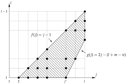
(a) The $\min\{m,n\}\geq l$ case

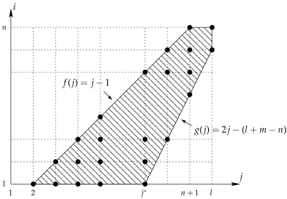
(b) The $\min\{m,n\}<l$ case

Figure 1: For each $j$, the black dots represent the $\alpha$’s that are freed by $\beta_{j}$. For each $i$, the number of black dots $c_{i}$ is the coefficient of $\alpha_{i}$. Thus, for $i\leq g(l)$, $c_{i}=\left\lfloor{g^{-1}(i)}\right\rfloor-\left\lceil{f^{-1}(i)}\right\rceil+1$; and for $i>g(l)$, $c_{i}=l-\left\lceil{f^{-1}(i)}\right\rceil+1$.

III-B The $\min\{m,n\}<l$ Case

Again, by the reciprocity property, we assume that $n\leq m$. However, we should study the $m\geq l$ case and the $m<l$ case separately. We start with the former case.

III-B1 The $n<l\leq m$ Case

From (4) and (6), we get the joint p.d.f. of $(\boldsymbol{\lambda},\boldsymbol{\mu})$

$$\begin{split}p_{\boldsymbol{\lambda},\boldsymbol{\mu}}(\boldsymbol{\lambda},\boldsymbol{\mu})&=B_{l,m,n}\prod_{i=1}^{l}\mu_{i}^{m-l}\prod_{i<j}^{l}{(\mu_{i}-\mu_{j})}\\ &\quad\cdot\prod_{i<j}^{n}{(\lambda_{i}-\lambda_{j})}\,\mathrm{Det}\left(\boldsymbol{\Xi}\right)\end{split}$$ (15)

where $B_{l,m,n}$ is the normalization factor. Same procedure as the previous case and Lemma 3 lead to the following asymptotical p.d.f. of $(\boldsymbol{\alpha},\boldsymbol{\beta})$

$$\begin{split}p_{\boldsymbol{\alpha},\boldsymbol{\beta}}(\boldsymbol{\alpha},\boldsymbol{\beta})&\doteq(\log{\mathsf{SNR}})^{l+n}\prod_{i=1}^{n}{\mathsf{SNR}}^{-(n-i+1)\alpha_{i}}\\ &\quad\cdot\prod_{i=1}^{n+1}{\mathsf{SNR}}^{-(l+m-n-i)\alpha_{i}}\prod_{i=n+2}^{l}{\mathsf{SNR}}^{-(l+m+1-2i)\alpha_{i}}\\ &\quad\cdot\prod_{i=1}^{n}\prod_{j=n+1}^{l}{\mathsf{SNR}}^{-(\alpha_{i}-\beta_{j})^{+}}\prod_{i<j}^{n}{\mathsf{SNR}}^{-(\alpha_{i}-\beta_{j})^{+}}\\ &\quad\cdot\exp\left(-\sum_{i=1}^{l}{\mathsf{SNR}}^{-\beta_{i}}\right)\exp\left(-\sum_{i=1}^{n}{\mathsf{SNR}}^{-(\alpha_{i}-\beta_{i})}\right).\end{split}$$

As before, we only consider $\beta_{i}\geq 0,\forall i$, and $\alpha_{i}\geq\beta_{i}$, for $i=1,\ldots,n$, in order that $p_{\boldsymbol{\alpha},\boldsymbol{\beta}}(\boldsymbol{\alpha},\boldsymbol{\beta})$ does not decay exponentially. Finally, the DMT $d(r)$ can be obtained by solving the optimization problem (10) with

$$\mathcal{O}(\boldsymbol{\alpha},\boldsymbol{\beta},r)\triangleq\left\{(\boldsymbol{\alpha},\boldsymbol{\beta}):\quad\sum_{i=1}^{n}(1-\alpha_{i})^{+}<r,{{\alpha_{1}\leq\cdots\leq\alpha_{n},\atop\beta_{1}\leq\cdots\leq\beta_{l}},\alpha_{i}\geq\beta_{i}\geq 0,\text{for}\ i=1,\ldots,n}\right\}$$

and

$$\begin{split}\epsilon(\boldsymbol{\alpha},\boldsymbol{\beta})=&\sum_{i=1}^{n}(n+1-i)\alpha_{i}+\sum_{i=1}^{n+1}(l+m-n-i)\beta_{i}\\ &\quad+\sum_{i=n+2}^{l}(l+m+1-2i)\beta_{i}+\sum_{i=1}^{n}\!\sum_{j=n+1}^{l}(\alpha_{i}-\beta_{j})^{+}\\ &\quad+\sum_{i<j}^{n}(\alpha_{i}-\beta_{j})^{+}.\end{split}$$ (16)

The optimization procedure is exactly the same as in the previous case. With the optimal $\beta_{j}$’s, we have

$$\epsilon(\boldsymbol{\alpha})=\sum_{i=1}^{n}(n-i+1+c_{i})\alpha_{i}$$ (17)

where $c_{i}$ can be found with the help of Fig. ​1(b). Finally, we have

$$\begin{split}\epsilon(\boldsymbol{\alpha})&=\sum_{i=1}^{l-(m-n)}\left(n+1-2i+\left\lfloor\frac{l+i+(m-n)}{2}\right\rfloor\right)\alpha_{i}\\ &\quad+\sum_{i=l-(m-n)+1}^{n}\left(n+l+1-2i\right)\alpha_{i}\end{split}$$

where the coefficient of $\alpha_{i}$ is non-negative and is non-increasing with $i$. Hence, the optimal solution is $\alpha_{i}^{*}=1,i=k+1,\ldots,l$ and $\alpha_{i}^{*}=0,i=1,\ldots,k$, from which we have

$$d(k)=(l-k)(n-k)-\left\lfloor\frac{\left[(n-(m-l)-k)^{+}\right]^{2}}{4}\right\rfloor.$$ (18)

III-B2 The $n\leq m<l$ Case

In this case, $\mu_{m+1}=\cdots=\mu_{l}=0$ with probability $1$. Let $\boldsymbol{\mu}\triangleq{\left[\mu_{1}\cdots\mu_{m}\right]}^{\scriptscriptstyle\mathsf{T}\!}$ be the vector of the nonzero eigenvalues of ${\boldsymbol{Q}}_{1}$. The conditional p.d.f. $p_{\boldsymbol{\lambda}|\boldsymbol{\mu}}(\boldsymbol{\lambda}|\boldsymbol{\mu})$ is given by Lemma 4. The p.d.f. of $\boldsymbol{\mu}$ being known from (6), we get the joint p.d.f. of $(\boldsymbol{\lambda},\boldsymbol{\mu})$ in exactly the same form as (15), except that $l$ and $m$ are interchanged. We have directly

$$d(k)=(m-k)(n-k)-\left\lfloor\frac{\left[(n-(l-m)-k)^{+}\right]^{2}}{4}\right\rfloor.$$ (19)

IV Diversity-Multiplexing Tradeoff of Double Scattering MIMO Channels

In this section, we study the DMT of a general double scattering channel, where the antenna and scatterer correlations $\boldsymbol{\Phi}_{\text{T}}$, $\boldsymbol{\Phi}_{\text{S}}$ and $\boldsymbol{\Phi}_{\text{R}}$ are non-trivial.

It is intuitive to expect that the DMT is independent of the correlation matrices, as long as they are not singular, since the DMT is an asymptotical performance measure. First of all, it is easy to show that the antenna correlations $\boldsymbol{\Phi}_{\text{T}}$ and $\boldsymbol{\Phi}_{\text{R}}$ do not affect the tradeoff. To see this, note that

$$\det(\mathbf{I}+{\mathsf{SNR}}{\boldsymbol{H}}{{\boldsymbol{H}}}^{\scriptscriptstyle{\dagger}\!}) =\det(\mathbf{I}+{\mathsf{SNR}}\boldsymbol{\Phi}_{\text{R}}^{1/2}{\boldsymbol{H}}_{2}\boldsymbol{\Phi}_{\text{S}}^{1/2}{\boldsymbol{H}}_{1}\boldsymbol{\Phi}_{\text{T}}{{\boldsymbol{H}}}^{\scriptscriptstyle{\dagger}\!}_{1}\boldsymbol{\Phi}_{\text{S}}^{1/2}{{\boldsymbol{H}}}^{\scriptscriptstyle{\dagger}\!}_{2}\boldsymbol{\Phi}_{\text{R}}^{1/2})$$

$$\doteq\det(\mathbf{I}+{\mathsf{SNR}}\boldsymbol{\Phi}_{\text{R}}^{1/2}{\boldsymbol{H}}_{2}\boldsymbol{\Phi}_{\text{S}}^{1/2}{\boldsymbol{H}}_{1}{{\boldsymbol{H}}}^{\scriptscriptstyle{\dagger}\!}_{1}\boldsymbol{\Phi}_{\text{S}}^{1/2}{{\boldsymbol{H}}}^{\scriptscriptstyle{\dagger}\!}_{2}\boldsymbol{\Phi}_{\text{R}}^{1/2})$$

$$\doteq\det(\mathbf{I}+{\mathsf{SNR}}{{\boldsymbol{H}}}^{\scriptscriptstyle{\dagger}\!}_{1}\boldsymbol{\Phi}_{\text{S}}^{1/2}{{\boldsymbol{H}}}^{\scriptscriptstyle{\dagger}\!}_{2}{\boldsymbol{H}}_{2}\boldsymbol{\Phi}_{\text{S}}^{1/2}{\boldsymbol{H}}_{1})$$

where $\boldsymbol{\Phi}_{\text{T}}$ and $\boldsymbol{\Phi}_{\text{R}}$ disappear in the high SNR analysis. Now, it remains to show that $\boldsymbol{\Phi}_{\text{S}}$ has no impact on the high SNR analysis. The following proposition confirms this statement.

Proposition 1

Let ${\boldsymbol{M}}$ be any $m\times n$ random matrix and ${\boldsymbol{T}}$ be any $m\times m$ non-singular matrix whose singular values satisfy $\sigma_{\min}({\boldsymbol{T}})\doteq\sigma_{\max}({\boldsymbol{T}})\doteq{\mathsf{SNR}}^{0}$. Define $q\triangleq\min\{m,n\}$ and $\boldsymbol{\tilde{M}}\triangleq{\boldsymbol{T}}{\boldsymbol{M}}$. Let $\sigma_{1}({\boldsymbol{M}})>\ldots>\sigma_{q}({\boldsymbol{M}})>0$ and $\sigma_{1}(\boldsymbol{\tilde{M}})>\ldots>\sigma_{q}(\boldsymbol{\tilde{M}})>0$ be the distinct ordered singular values of ${\boldsymbol{M}}$ and $\boldsymbol{\tilde{M}}$, Then, we have

$$\sigma_{i}(\boldsymbol{\tilde{M}})\doteq\sigma_{i}({\boldsymbol{M}}),\quad\forall i.$$

Proof:

For $m\geq n$, we consider the left polar decomposition ${\boldsymbol{M}}={\boldsymbol{U}}{\boldsymbol{M}}_{0}$, where ${\boldsymbol{U}}$ is a $m\times n$ matrix with orthonormal columns and ${\boldsymbol{M}}_{0}$ a $n\times n$ positive definite matrix with $\sigma_{i}({\boldsymbol{M}})=\sigma_{i}({\boldsymbol{M}}_{0})$ for $i=1,\ldots,n$. Let ${\boldsymbol{T}}{\boldsymbol{U}}={\boldsymbol{V}}{\boldsymbol{T}}_{0}$ be the left polar decomposition of ${\boldsymbol{T}}{\boldsymbol{U}}$. Then, we have $\sigma_{i}(\boldsymbol{\tilde{M}})=\sigma_{i}({\boldsymbol{T}}_{0}{\boldsymbol{M}}_{0})$ for $i=1,\ldots,n$.

For $m<n$, we make a right polar decomposition ${\boldsymbol{M}}={\boldsymbol{M}}_{0}{{\boldsymbol{U}}}^{\scriptscriptstyle{\dagger}\!}$ , where ${\boldsymbol{U}}$ is a $n\times m$ matrix with orthonormal columns and ${\boldsymbol{M}}_{0}$ a $m\times m$ positive definite matrix with $\sigma_{i}({\boldsymbol{M}})=\sigma_{i}({\boldsymbol{M}}_{0})$ for $i=1,\ldots,n$. Then, we have $\sigma_{i}(\boldsymbol{\tilde{M}})=\sigma_{i}({\boldsymbol{T}}_{0}{\boldsymbol{M}}_{0})$ for $i=1,\ldots,n$ with ${\boldsymbol{T}}_{0}\triangleq{\boldsymbol{T}}$.

In both cases, the original problem is equivalent to showing that

$$\sigma_{i}({\boldsymbol{T}}_{0}{\boldsymbol{M}}_{0})\doteq\sigma_{i}({\boldsymbol{M}}_{0}),\quad\text{for}\ i=1,\ldots,q,$$

with ${\boldsymbol{T}}_{0}$ and ${\boldsymbol{M}}_{0}$ now invertible. Let ${\boldsymbol{A}}$ and ${\boldsymbol{B}}$ in Lemma 5 be ${\boldsymbol{T}}_{0}$ and ${\boldsymbol{M}}_{0}$, respectively. By applying (28) and (29) of appendix, we have

$$\sigma_{i}({\boldsymbol{M}}_{0})\sigma_{m}({\boldsymbol{T}}_{0})\leq\sigma_{i}(\boldsymbol{\tilde{M}})\leq\sigma_{i}({\boldsymbol{M}}_{0})\sigma_{1}({\boldsymbol{T}}_{0}),$$

from which we prove the proposition since $\sigma_{1}({\boldsymbol{T}}_{0})\doteq\sigma_{m}({\boldsymbol{T}}_{0})\doteq{\mathsf{SNR}}^{0}$ and $\sigma_{i}({\boldsymbol{M}})=\sigma_{i}({\boldsymbol{M}}_{0})$. ∎

This proposition says that any invertible transformation with bounded (asymptotically in high SNR regime) eigenvalues does not change the asymptotical p.d.f. of the singular values of a random matrix. According to this proposition, we know that the singular values of $\boldsymbol{\Phi}_{\text{S}}^{1/2}{\boldsymbol{H}}_{1}$ have the same asymptotical p.d.f. as the ones of ${\boldsymbol{H}}_{1}$, which leads to the main result of this work.

Theorem 3

For a $(n_{\text{T}},n_{\text{S}},n_{\text{R}})$ double scattering MIMO channel (1) with ${\boldsymbol{H}}$ defined in (2), the diversity-multiplexing tradeoff is a piecewise-linear function connecting the points $(k,d(k)),k=0,\ldots,M$ with $d(k)$ being defined in (9), where $(M,N,L)$ is the ordered version of $(n_{\text{T}},n_{\text{S}},n_{\text{R}})$ with $M\leq N\leq L$.

Proof:

This is a direct consequence of Theorem 2, since the eigenvalues of $(\boldsymbol{\Phi}_{\text{S}}^{1/2}{\boldsymbol{H}}_{1}){(\boldsymbol{\Phi}_{\text{S}}^{1/2}{\boldsymbol{H}}_{1})}^{\scriptscriptstyle{\dagger}\!}$ have the same asymptotical p.d.f. as that of ${\boldsymbol{H}}_{1}{{\boldsymbol{H}}}^{\scriptscriptstyle{\dagger}\!}_{1}$. ∎

Note that all observations in Remark 1 apply for the general double scattering MIMO channel. In particular, the optimality condition $L+1\geq M+N$ in observation 4 of Remark 1 in terms of $(n_{\text{T}},n_{\text{S}},n_{\text{R}})$ is

$$2\max\left\{n_{\text{T}},n_{\text{S}},n_{\text{R}}\right\}+1\geq n_{\text{T}}+n_{\text{S}}+n_{\text{R}},$$

which is also the condition under which the maximum channel diversity order $n_{\text{T}}n_{\text{S}}n_{\text{R}}/\max\left\{n_{\text{T}},n_{\text{S}},n_{\text{R}}\right\}$ is achieved. Moreover, this theorem implies that antenna or scatterer correlation does not, indeed, have any impact on the DMT of a double scattering channel, as long as the correlation matrices are non-singular. Finally, in the singular correlation matrices case, it is straightfoward to show that Theorem 3 is still true, but with $(n_{\text{T}},n_{\text{S}},n_{\text{R}})$ replaced by $(n_{\text{T}}^{\prime},n_{\text{S}}^{\prime},n_{\text{R}}^{\prime})$, the respective ranks of the correlation matrices.

V Conclusion

We studied, in this paper, the DMT of a double scattering MIMO channel and showed that, as long as the correlation matrices are non singular, it is equal to the DMT of a Rayleigh MIMO product channel. This DMT is always lower than the one of a single scattering ($n_{\text{T}}\times n_{\text{S}}$, $n_{\text{S}}\times n_{\text{R}}$ or $n_{\text{T}}\times n_{\text{R}}$) MIMO channel and it is equal to that one for certain values of the channel parameters. This result is not only interesting for itself, but it also helps to the calculation of the DMT of MIMO Amplify-and-Forward [9] cooperative channels as the relayed link can be seen as a Rayleigh MIMO product channel.

Lemma 2

$$\begin{split}&\mathrm{Det}\left[\exp\left(-{\mathsf{SNR}}^{-(\alpha_{j}-\beta_{i})}\right)\right]_{i,j=1}^{l}\\ &\quad\doteq\exp\left(-\sum_{i=1}^{l}{\mathsf{SNR}}^{-(\alpha_{i}-\beta_{i})}\right){\mathsf{SNR}}^{-\sum_{i<j}^{l}(\alpha_{i}-\beta_{j})^{+}}.\end{split}$$ (20)

Proof:

Let us define $D_{l}\triangleq\mathrm{Det}\left[\exp\left(-{\mathsf{SNR}}^{-(\alpha_{j}-\beta_{i})}\right)\right]_{i,j=1}^{l}$ and we have

$$\begin{split}D_{l}&=\mathrm{Det}\begin{bmatrix}e^{-{\mathsf{SNR}}^{-(\alpha_{1}-\beta_{1})}+{\mathsf{SNR}}^{-(\alpha_{l}-\beta_{1})}}&\cdots&e^{-{\mathsf{SNR}}^{-(\alpha_{l-1}-\beta_{1})}+{\mathsf{SNR}}^{-(\alpha_{l}-\beta_{1})}}&1\\ \vdots&\ddots&\vdots&\vdots\\ e^{-{\mathsf{SNR}}^{-(\alpha_{1}-\beta_{l})}+{\mathsf{SNR}}^{-(\alpha_{l}-\beta_{l})}}&\cdots&e^{-{\mathsf{SNR}}^{-(\alpha_{l-1}-\beta_{l})}+{\mathsf{SNR}}^{-(\alpha_{l}-\beta_{l})}}&1\end{bmatrix}e^{-\sum_{i}{\mathsf{SNR}}^{-(\alpha_{l}-\beta_{i})}}\\ &\doteq\mathrm{Det}\begin{bmatrix}e^{-{\mathsf{SNR}}^{-(\alpha_{1}-\beta_{1})}}-e^{-{\mathsf{SNR}}^{-(\alpha_{1}-\beta_{l})}}&\cdots&e^{-{\mathsf{SNR}}^{-(\alpha_{l-1}-\beta_{1})}}-e^{-{\mathsf{SNR}}^{-(\alpha_{l-1}-\beta_{l})}}&0\\ \vdots&\ddots&\vdots&\vdots\\ e^{-{\mathsf{SNR}}^{-(\alpha_{1}-\beta_{l-1})}}-e^{-{\mathsf{SNR}}^{-(\alpha_{1}-\beta_{l})}}&\cdots&e^{-{\mathsf{SNR}}^{-(\alpha_{l-1}-\beta_{l-1})}}-e^{-{\mathsf{SNR}}^{-(\alpha_{l-1}-\beta_{l})}}&0\\ e^{-{\mathsf{SNR}}^{-(\alpha_{1}-\beta_{l})}}&\cdots&e^{-{\mathsf{SNR}}^{-(\alpha_{l-1}-\beta_{l})}}&1\end{bmatrix}e^{-{\mathsf{SNR}}^{-(\alpha_{l}-\beta_{l})}}\\ &\doteq\mathrm{Det}\begin{bmatrix}e^{-{\mathsf{SNR}}^{-(\alpha_{1}-\beta_{1})}}\left(1-e^{-{\mathsf{SNR}}^{-(\alpha_{1}-\beta_{l})}}\right)&\cdots&e^{-{\mathsf{SNR}}^{-(\alpha_{l-1}-\beta_{1})}}\left(1-e^{-{\mathsf{SNR}}^{-(\alpha_{l-1}-\beta_{l})}}\right)\\ \vdots&\ddots&\vdots\\ e^{-{\mathsf{SNR}}^{-(\alpha_{1}-\beta_{l-1})}}\left(1-e^{-{\mathsf{SNR}}^{-(\alpha_{1}-\beta_{l})}}\right)&\cdots&e^{-{\mathsf{SNR}}^{-(\alpha_{l-1}-\beta_{l-1})}}\left(1-e^{-{\mathsf{SNR}}^{-(\alpha_{l-1}-\beta_{l})}}\right)\end{bmatrix}e^{-{\mathsf{SNR}}^{-(\alpha_{l}-\beta_{l})}}\\ &=e^{-{\mathsf{SNR}}^{-(\alpha_{l}-\beta_{l})}}\prod_{i=1}^{l-1}\left(1-e^{-{\mathsf{SNR}}^{-(\alpha_{i}-\beta_{l})}}\right)D_{l-1}\end{split}$$

where the equations are obtained by iterating the identity ${\mathsf{SNR}}^{-a}\pm{\mathsf{SNR}}^{-b}\doteq{\mathsf{SNR}}^{-a}$ for $a<b$. Since $1-e^{-x}\approx x$ for $x$ close to $0^{+}$, we have $1-e^{-{\mathsf{SNR}}^{-(\alpha_{i}-\beta_{l})}}\doteq{\mathsf{SNR}}^{-(\alpha_{i}-\beta_{l})}$ if $\alpha_{i}>\beta_{l}$ and $1-e^{-{\mathsf{SNR}}^{-(\alpha_{i}-\beta_{l})}}\doteq{\mathsf{SNR}}^{0}$ otherwise. As shown in the recursive relation above, we must have $\alpha_{i}\geq\beta_{i},\forall i$, in order that $D_{l}$ does not decay exponentially. Thus, we have $D_{l}\doteq{\mathsf{SNR}}^{-\sum_{i<l}(\alpha_{i}-\beta_{l})^{+}}D_{l-1}$, and in a recursive manner, we get (20).

∎

Lemma 3

$$\begin{split}\mathrm{Det}\left(\boldsymbol{\Xi}\right)&\doteq\prod_{i=1}^{n+1}{\mathsf{SNR}}^{-(l+m-n-i)\alpha_{i}}\prod_{i=n+2}^{l}{\mathsf{SNR}}^{-(l+m+1-2i)\alpha_{i}}\\ &\quad\cdot\prod_{i=1}^{n}\prod_{j=n+1}^{l}{\mathsf{SNR}}^{-(\alpha_{i}-\beta_{j})^{+}}\prod_{i<j}^{n}{\mathsf{SNR}}^{-(\alpha_{i}-\beta_{j})^{+}}\\ &\quad\cdot\exp\left(-\sum_{i=1}^{n}{\mathsf{SNR}}^{-(\alpha_{i}-\beta_{i})}\right).\end{split}$$

Proof:

First, we have

$$\mathrm{Det}{(\boldsymbol{\Xi})}=\prod_{i=1}^{l}\mu_{i}^{l-n-1}\mathrm{Det}\begin{bmatrix}\mu_{1}^{-(l-n-1)}&\cdots&1&e^{-\lambda_{1}/\mu_{1}}&\cdots&e^{-\lambda_{n}/\mu_{1}}\\ \vdots&\ddots&\vdots&\vdots&\ddots&\vdots\\ \mu_{l}^{-(l-n-1)}&\cdots&1&e^{-\lambda_{1}/\mu_{l}}&\cdots&e^{-\lambda_{n}/\mu_{l}}\\ \end{bmatrix}.$$ (21)

Then, let us denote the determinant in the right hand side of (21) as $D$ and we rewrite it as

$$D =\mathrm{Det}\begin{bmatrix}d_{1,l}^{(l-n-1)}&\cdots&0&e^{-\lambda_{1}/\mu_{1}}-e^{-\lambda_{1}/\mu_{l}}&\cdots&e^{-\lambda_{n}/\mu_{1}}-e^{-\lambda_{n}/\mu_{l}}\\ \vdots&\ddots&\vdots&\vdots&\ddots&\vdots\\ d_{l-1,l}^{(l-n-1)}&\cdots&0&e^{-\lambda_{1}/\mu_{l-1}}-e^{-\lambda_{1}/\mu_{l}}&\cdots&e^{-\lambda_{n}/\mu_{l-1}}-e^{-\lambda_{n}/\mu_{l}}\\ \mu_{l}^{-(l-n-1)}&\cdots&1&e^{-\lambda_{1}/\mu_{l}}&\cdots&e^{-\lambda_{n}/\mu_{l}}\\ \end{bmatrix}$$ (22)

$$\doteq\mathrm{Det}\begin{bmatrix}d_{1,l}^{(l-n-1)}&\cdots&d_{1,l}^{(1)}&e^{-\lambda_{1}/\mu_{1}}&\cdots&e^{-\lambda_{n}/\mu_{1}}\\ \vdots&\ddots&\vdots&\vdots&\ddots&\vdots\\ d_{l-1,l}^{(l-n-1)}&\cdots&d_{l-1,l}^{(1)}&e^{-\lambda_{1}/\mu_{l-1}}&\cdots&e^{-\lambda_{n}/\mu_{l-1}}\\ \end{bmatrix}\prod_{i=1}^{n}\left(1-e^{-\lambda_{i}/\mu_{l}}\right)$$ (23)

where $d_{i,j}^{(k)}\triangleq\mu_{i}^{-k}-\mu_{j}^{-k}$ and the product term in (23) is obtained since $1-e^{-(\lambda_{i}/\mu_{l}-\lambda_{i}/\mu_{j})}\doteq 1-e^{-\lambda_{i}/\mu_{l}}$ for all $j<l$. Let us denote the determinant in (23) as $D_{l}$. Then, by multiplying the first column in $D_{l}$ with $\mu_{l}^{l-n-1}$ and noting that $\mu_{l}^{l-n-1}d_{i,l}^{(l-n-1)}=1-\left(\displaystyle\frac{\mu_{l}}{\mu_{i}}\right)^{l-n-1}\approx 1$, the first column of $D_{l}$ becomes all $1$. Now, by eliminating the first $l-2$ “$1$”s of the first column by substracting all rows by the last row as in (22) and (23), we have $\mu_{l}^{l-n-1}D_{l}\doteq\prod_{i=1}^{n}\left(1-e^{-\lambda_{i}/\mu_{l}}\right)D_{l-1}$. By continuing reducing the dimension, we get

$$\begin{split}\mathrm{Det}(\boldsymbol{\Xi})&\doteq\mathrm{Det}\left[e^{-\lambda_{j}/\mu_{i}}\right]_{i,j=1}^{n}\prod_{i=1}^{n+1}\mu_{i}^{l-n-1}\prod_{i=n+2}^{l}\mu_{i}^{l-i}\\ &\quad\cdot\prod_{i=1}^{n}\prod_{j=n+1}^{l}\left(1-e^{-\lambda_{i}/\mu_{j}}\right)\end{split}$$

from which we prove the lemma, by applying (20). ∎

Lemma 4

Let ${\boldsymbol{W}}$ be a central complex Wishart matrix ${\boldsymbol{W}}\sim\mathcal{W}_{m}(n,\boldsymbol{\Sigma})$ with $n<m$, where the ordered eigenvalues of $\boldsymbol{\Sigma}$ are $\mu_{1}>\ldots>\mu_{l}>\mu_{l+1}=\ldots=\mu_{m}=0$ with $l\geq n$. The joint p.d.f. of the ordered positive eigenvalues $\lambda_{1}>\ldots>\lambda_{n}$ of ${\boldsymbol{W}}$ equals

$$G_{m,n}\mathrm{Det}(\boldsymbol{\Xi}_{l})\prod_{i<j}^{l}\frac{1}{(\mu_{i}-\mu_{j})}\prod_{i<j}^{n}(\lambda_{i}-\lambda_{j})$$ (24)

with

$$\boldsymbol{\Xi}_{l}\triangleq\begin{bmatrix}1&\mu_{1}&\cdots&\mu_{1}^{l-n-1}&\mu_{1}^{l-n-1}e^{-\frac{\lambda_{1}}{\mu_{1}}}&\cdots&\mu_{1}^{l-n-1}e^{-\frac{\lambda_{n}}{\mu_{1}}}\\ \vdots&\vdots&\ddots&\vdots&\vdots&\ddots&\vdots\\ 1&\mu_{l}&\cdots&\mu_{l}^{l-n-1}&\mu_{l}^{l-n-1}e^{-\frac{\lambda_{1}}{\mu_{l}}}&\cdots&\mu_{l}^{l-n-1}e^{-\frac{\lambda_{n}}{\mu_{l}}}\end{bmatrix}.$$ (25)

Proof:

We can prove it by successively applying the l’Hospital rule with $\mu_{m},\ldots,\mu_{l+1}\to 0$ on the expression in (4). Let us prove by induction that

$$\lim_{\mu_{l+1},\ldots,\mu_{m}\to 0}\frac{\mathrm{Det}(\boldsymbol{\Xi})}{\prod_{i<j}^{m}(\mu_{i}-\mu_{j})}=\frac{\mathrm{Det}(\boldsymbol{\Xi}_{l})}{\prod_{i<j}^{l}(\mu_{i}-\mu_{j})}.$$ (26)

For $l=m-1$, (26) is obviously true. Then, assuming that (26) holds for given $l$, then, as long as $l-1\geq n$, we have

$$\lim_{\mu_{l},\ldots,\mu_{m}\to 0}\frac{\mathrm{Det}(\boldsymbol{\Xi})}{\prod_{i<j}^{m}(\mu_{i}-\mu_{j})} = \lim_{\mu_{l}\to 0}\frac{\mathrm{Det}(\boldsymbol{\Xi}_{l})}{\prod_{i<j}^{l}(\mu_{i}-\mu_{j})}$$ (27)

$$= \frac{\mathrm{Det}(\boldsymbol{\Xi}_{l-1})}{\prod_{i<j}^{l-1}(\mu_{i}-\mu_{j})}$$

where (27) is deduced from (26). ∎

Lemma 5

Let ${\boldsymbol{A}}$ and ${\boldsymbol{B}}$ be two $m\times m$ non-singular matrices. For any $n\times n$ matrix ${\boldsymbol{M}}$, let $\sigma_{i}({\boldsymbol{M}})$ be the $i$th largest singular value of ${\boldsymbol{M}}$ and $\eta_{i}{({\boldsymbol{M}})}$ be the $i$th smallest one (i.e., $\sigma_{i}({\boldsymbol{M}})=\eta_{n+1-i}({\boldsymbol{M}})$). Then, we have

$$\sigma_{i+j-1}({\boldsymbol{A}}{\boldsymbol{B}}) \leq \sigma_{i}({\boldsymbol{A}})\,\sigma_{j}({\boldsymbol{B}})$$ (28)

$$\eta_{i+j-1}({\boldsymbol{A}}{\boldsymbol{B}}) \geq \eta_{i}({\boldsymbol{A}})\,\eta_{j}({\boldsymbol{B}})$$ (29)

for $1\leq\{i,j\}\leq m$ and $i+j\leq m+1$.

Proof:

Let ${\boldsymbol{A}}{\boldsymbol{B}}={\boldsymbol{U}}{\boldsymbol{Q}}$ be the left polar decomposition of ${\boldsymbol{A}}{\boldsymbol{B}}$ with ${\boldsymbol{U}}$ unitary and ${\boldsymbol{Q}}$ positive definite. Then, we have ${\boldsymbol{Q}}={{\boldsymbol{U}}}^{\scriptscriptstyle{\dagger}\!}{\boldsymbol{A}}{\boldsymbol{B}}$ and $\sigma_{i}({\boldsymbol{Q}})=\sigma_{i}({\boldsymbol{A}}{\boldsymbol{B}}),\forall i$. The quadratic form ${{\boldsymbol{x}}}^{\scriptscriptstyle{\dagger}\!}\,{\boldsymbol{Q}}{\boldsymbol{x}}$ can be bounded as

$$\begin{split}\left|{{\boldsymbol{x}}}^{\scriptscriptstyle{\dagger}\!}{\boldsymbol{Q}}{\boldsymbol{x}}\right|^{2}&=\left|{\left({{\boldsymbol{A}}}^{\scriptscriptstyle{\dagger}\!}{\boldsymbol{U}}{\boldsymbol{x}}\right)}^{\scriptscriptstyle{\dagger}\!}\left({\boldsymbol{B}}{\boldsymbol{x}}\right)\right|^{2}\\ &\leq\left\|{{{\boldsymbol{A}}}^{\scriptscriptstyle{\dagger}\!}\,{\boldsymbol{U}}{\boldsymbol{x}}}\right\|^{2}\left\|{{\boldsymbol{B}}{\boldsymbol{x}}}\right\|^{2}\\ &=\left({{\boldsymbol{x}}}^{\scriptscriptstyle{\dagger}\!}_{1}{\boldsymbol{Q}}_{{\boldsymbol{A}}}{\boldsymbol{x}}_{1}\right)\left({{\boldsymbol{x}}}^{\scriptscriptstyle{\dagger}\!}\,{\boldsymbol{Q}}_{{\boldsymbol{B}}}{\boldsymbol{x}}\right)\end{split}$$ (30)

where ${\boldsymbol{x}}_{1}\triangleq{\boldsymbol{U}}{\boldsymbol{x}}$, ${\boldsymbol{Q}}_{{\boldsymbol{A}}}\triangleq{\boldsymbol{A}}{{\boldsymbol{A}}}^{\scriptscriptstyle{\dagger}\!}$ and ${\boldsymbol{Q}}_{{\boldsymbol{B}}}\triangleq{\boldsymbol{B}}{{\boldsymbol{B}}}^{\scriptscriptstyle{\dagger}\!}$. The eigenvalue decomposition of ${\boldsymbol{Q}}_{{\boldsymbol{A}}}$ and ${\boldsymbol{Q}}_{{\boldsymbol{B}}}$ gives

$${\boldsymbol{Q}}_{{\boldsymbol{A}}} =\sum_{i=1}^{m}\sigma_{i}^{2}({\boldsymbol{A}}){\boldsymbol{z}}_{i}{{\boldsymbol{z}}}^{\scriptscriptstyle{\dagger}\!}_{i}\quad\text{and}$$

$${\boldsymbol{Q}}_{{\boldsymbol{B}}} =\sum_{i=1}^{m}\sigma_{i}^{2}({\boldsymbol{B}}){\boldsymbol{y}}_{i}{{\boldsymbol{y}}}^{\scriptscriptstyle{\dagger}\!}_{i}$$

where ${\boldsymbol{z}}_{i}$ and ${\boldsymbol{y}}_{i}$ are eigenvectors of ${\boldsymbol{Q}}_{{\boldsymbol{A}}}$ and ${\boldsymbol{Q}}_{{\boldsymbol{B}}}$, respectively. Now, taking ${\boldsymbol{x}}_{k}={{\boldsymbol{U}}}^{\scriptscriptstyle{\dagger}\!}{\boldsymbol{z}}_{k}$ for $k=1,\ldots,i-1$ and ${\boldsymbol{x}}_{k}={\boldsymbol{y}}_{k-i+1}$ for $k=i,\ldots,i+j-2$, we have, $\forall{\boldsymbol{x}}\perp{\boldsymbol{x}}_{k}$ for $k=1,\ldots,i+j-2$,

$${\left({\boldsymbol{U}}{\boldsymbol{x}}\right)}^{\scriptscriptstyle{\dagger}\!}\,{\boldsymbol{Q}}_{{\boldsymbol{A}}}\left({\boldsymbol{U}}{\boldsymbol{x}}\right) \leq\sigma_{i}^{2}({\boldsymbol{A}})\left\|{{\boldsymbol{x}}}\right\|^{2}$$ (31)

$${{\boldsymbol{x}}}^{\scriptscriptstyle{\dagger}\!}\,{\boldsymbol{Q}}_{{\boldsymbol{B}}}{\boldsymbol{x}} \leq\sigma_{j}^{2}({\boldsymbol{B}})\left\|{{\boldsymbol{x}}}\right\|^{2}.$$ (32)

From (30), (31) and (32) and the Courant-Fischer theorem [10], we get

$$\sigma_{i}^{2}({\boldsymbol{A}}{\boldsymbol{B}})\leq\max_{{\boldsymbol{x}}\perp\,{\boldsymbol{x}}_{1},\ldots,{\boldsymbol{x}}_{i+j-2}}\frac{\left|{{\boldsymbol{x}}}^{\scriptscriptstyle{\dagger}\!}\,{\boldsymbol{Q}}{\boldsymbol{x}}\right|^{2}}{\left\|{{\boldsymbol{x}}}\right\|^{4}}\leq\sigma_{i}^{2}({\boldsymbol{A}})\sigma_{j}^{2}({\boldsymbol{B}}),$$

from which we have (28).

Note that for any invertible matrix ${\boldsymbol{M}}$, we have $\eta_{i}({\boldsymbol{M}})=\sigma_{i}^{-1}({{\boldsymbol{M}}}^{\scriptscriptstyle-1\!})$. By applying this equality and using the inequality (28), it is straightfoward to get (29) after some simple manipulations.

∎

References

- [1] J. Foschini, G. Golden, R. Valenzuela, and P. Wolniansky, “Simplified processing for high spectral efficiency wireless communication employing multi-element arrays,” IEEE J. Select. Areas Commun., vol. 17, pp. 1841–1852, Nov. 1999.
- [2] E. Telatar, “Capacity of multi-antenna Gaussian channels,” Europ. Trans. Telecommun., ETT, vol. 10, no. 6, pp. 585–596, Nov. 1999.
- [3] L. Zheng and D. N. C. Tse, “Diversity and multiplexing: A fundamental tradeoff in multiple-antenna channels,” IEEE Trans. Inform. Theory, vol. 49, no. 5, pp. 1073–1096, May 2003.
- [4] D. Gesbert, H. Bölcskei, D. A. Gore, and A. J. Paulraj, “Outdoor MIMO wireless channels: Models and performance prediction,” IEEE Trans. Commun., vol. 50, pp. 1926–1934, Dec. 2002.
- [5] A. T. James, “Distributions of matrix variates and latent roots derived from normal samples,” Annals of Math. Statistics, vol. 35, pp. 475–501, 1964.
- [6] H. Gao and P. J. Smith, “A determinant representation for the distribution of quadratic forms in complex normal vectors,” J. Multivariate Analysis, vol. 73, pp. 155–165, May 2000.
- [7] S. H. Simon, A. L. Moustakas, and L. Marinelli, “Capacity and character expansions: Moment generating function and other exact results for MIMO correlated channels,” 2004. [Online]. Available: http://mars.bell-labs.com/cm/ms/what/mars/papers/simon˙mgf/simon.pdf
- [8] A. M. Tulino and S. Verdu, “Random matrix theory and wireless communications,” Foundations and Trends in Communications and Information Theory, vol. 1, no. 1, pp. 1–182, 2004.
- [9] S. Yang and J.-C. Belfiore, “Optimal space-time codes for the MIMO amplify-and-forward cooperative channel,” Sept. 2005, submitted to IEEE Trans. Inform. Theory. [Online]. Available: http://fr.arxiv.org/pdf/cs.IT/0509006
- [10] R. A. Horn and C. R. Johnson, Matrix Analysis. New York: Cambridge, 1985.