A General Framework for Scalability and Performance Analysis of DHT Routing Systems

Abstract

In recent years, many DHT-based P2P systems have been proposed, analyzed, and certain deployments have reached a global scale with nearly one million nodes. One is thus faced with the question of which particular DHT system to choose, and whether some are inherently more robust and scalable. Toward developing such a comparative framework, we present the reachable component method (RCM) for analyzing the performance of different DHT routing systems subject to random failures. We apply RCM to five DHT systems and obtain analytical expressions that characterize their routability as a continuous function of system size and node failure probability. An important consequence is that in the large-network limit, the routability of certain DHT systems go to zero for any non-zero probability of node failure. These DHT routing algorithms are therefore unscalable, while some others, including Kademlia, which powers the popular eDonkey P2P system, are found to be scalable.

1 Introduction

Developing scalable and fault tolerant systems to leverage and utilize the shared resources of distributed computers has been an important research topic since the dawn of computer networking. In recent years, the popularity and wide deployment of peer-to-peer (P2P) systems has inspired the development of distributed hash tables (DHTs). DHTs typically offer scalable $O(\log n)$ routing latency and efficient lookup interface. According to a recent study [12], the DHT based file-sharing network eDonkey is emerging as one of the largest P2P systems with millions of users and accounting for the largest fraction of P2P traffic, while P2P traffic currently accounts for 60% of the total Internet bandwidth. Given the transient nature of P2P users, analyzing and understanding the robustness of DHT routing algorithms in the asymptotic system size limit under unreliable environments become essential.

In the past few years, there has been a growing number of newly proposed DHT routing algorithms. However, in the DHT routing literature, there have been few papers that provide a general analytical framework to compare across the myriad routing algorithms. In this paper, we develop a method to analyze the performance and scalability of different DHT routing systems under random failures of nodes. We would like to emphasize that we intend to analyze the performance of the basic routing geometry and protocol. In a real system implementation, there is no doubt that a system designer have many optional features, such as additional sequential neighbors, to provide improved fault tolerance. Nevertheless, the analysis of the basic routing geometry will give us more insights and good guidelines to compare among systems.

In this paper, we investigate the routing performance of five DHT systems with uniform node failure probability $q$. Such a failure model, also known as the static resilience model, is assumed in the simulation study done by Gummadi et al. [2]. A static failure model is well suited for analyzing performance in the shorter time scale. In a DHT, very fast detection of faults is generally possible through means such as TCP timeouts or keep-alive messages, but establishing new connections to replace the faulty nodes is more time and resource consuming. The applicability of the results derived from this static model to dynamic situations, such as churn, is currently under study.

Intuitively, as the node failure probability $q$ increases, the routing performance of the system will worsen. A quantitative metric, called routability is needed to characterize the routing performance of a DHT system under random failure:

Definition 1

The routability of a DHT routing system is the expected number of routable pairs of nodes divided by the expected number of possible pairs among the surviving nodes. In other words, it is the fraction of survived routing paths in the system. In general, routability is a function of the node failure probability $q$ and system size $N$.

As the DHT-based eDonkey is reaching global scale, it is important to study how DHT systems perform as the number of nodes reaches millions or even billions. In fact, we know from site percolation theory[15], that if $q>(1-p_{c})$, where $p_{c}$ is called the percolation threshold of the underlying network, then the network will get fragmented into very small-size connected components and for large enough network size. As a result, the routability of the network will approach zero for such failure probability due to the lack of connectivity. However, because of how messages get routed as specified by the underlying routing protocol, all pairs belonging to the same connected component need not be reachable under failure.

In general, the size of the connected components do not directly give us the routability of the subnetworks. Hence, one needs to develop a framework different from the well-known framework of percolation. As a result, this work investigates DHT routability under the random failure model for both finite system sizes and the infinite limit. We will define the scalability of a routing system as follows:

Definition 2

A DHT routing system is said to be scalable if and only if its routability converges to a nonzero value as the system size goes to infinity for a nonzero failure probability $q$. Mathematically, it is defined as follows:

$$\lim_{N\rightarrow\infty}r(N,q)>0\ \ for\ 0<q<1-p_{c}$$

where $r(N,q)$ denotes the routability of the system as a function of system size $N$ and failure probability $q$. Similarly, the system is said to be unscalable if and only if its routability converges to zero as the system size goes to infinity for a nonzero failure probability $q$:

$$\lim_{N\rightarrow\infty}r(N,q)=0\ \ for\ 0<q<1-p_{c}$$

We want to emphasize that in a real implementation, there are many system parameters that the system designer can specify, such as the number of near neighbors or sequential neighbors. As a result, the designer can always add enough sequential neighbors to achieve an acceptable routability under reasonable node failure probability for a maximum network size that exceeds the expected number of nodes that will participate in the system. The scalability definition is provided for examining the theoretical asymptotic behavior of DHT routing systems, not for claiming a DHT system is unsuitable for any large-scale deployment.

Having specified the definition of the key metrics, we will present the reachable component method (RCM), a simple yet effective method for analyzing DHT routing performance under random failure. We apply the RCM method to analyze the basic routing algorithms used in the following five DHT systems: Symphony [10], Kademlia [11], Chord [16], CAN [14] and Plaxton routing based systems [13]. For all algorithms except Chord routing, we derive the analytical expression for each algorithm’s routability under random failure, while an analytical expression for a tight lower bound is obtained for Chord routing. In fact, our analytical results match the simulation results carried out in [2], where different DHT systems were simulated and the percentage of failed paths (i.e., 1-routability) was estimated for $N=2^{16}$, as illustrated in Fig. 6. In addition, we also derive the asymptotic performance of the routing algorithm under failure as the system scales.

One interesting finding of this paper is that under random failure, the basic DHT routing systems can be classified into two classes: scalable and unscalable. For example, the XOR routing scheme of Kademlia is found to be scalable, since the routability of the system under nonzero probability of failure converges very fast to a positive limit even as the size of the system tends to infinity. This is consistent with the observation that the Kademlia-based popular P2P network eDonkey is able to scale to millions of nodes. In contrast, as the system scales, the routability of Symphony’s routing scheme is found to quickly converge to zero for any failure probability greater than zero. Thus, the basic routing system for Symphony is found to be unscalable. However, as briefly discussed above in this section, a system designer for Symphony can specify enough near neighbors to guarantee an acceptable routability in the system for a maximum network size and a reasonable failure probability $q$.

The rest of this paper is organized as follows. In section 2, we discuss previous work on the fault tolerance of P2P routing systems. In section 3, we will give an overview of the DHT routing systems that we intend to analyze. In section 4, we present the reachable component method (RCM) and apply the RCM method on several DHT systems. In section 5, we examine the scalability of DHT routing systems. In section 6, we give our concluding remarks.

2 Related Work

The study of robustness in routing networks has grown in the past few years with researchers simulating failure conditions in DHT-based systems. Gummadi et al.[2] showed through simulation results that the routing geometry of each system has a large effect on the network’s static resilience to random failures. In addition, there have been research work done in the area of analyzing and simulating dynamic failure conditions (i.e. churn) in DHT systems [8, 7, 5].

Theory work has been done to predict the performance of DHT systems under a static failure model. The two main approaches thus far have been graph theoretic methods[1, 9, 6] and Markov processes[17]. Most analytical work to date has dealt with one or two routing algorithms to which their respective methods are well-suited but have not provided comparisons across a large fraction of the DHT algorithms. Angel et al. [1] use percolation theory to place tight bounds on the critical failure probability that can support efficient routing on both hypercube and $d$-dimensional mesh topologies. By efficient they mean that it is possible to route between two nodes with time complexity on the order of the network diameter. While this method predicts the point at which the network becomes virtually unusable, it does not allow the detailed characterization of routability as a function of the failure probability. In contrast, the reachable component method (RCM) method exploits the geometries of DHT routing networks and leads to simple analytical results that predict routing performance for arbitrary network sizes and failure probabilities.

3 Overview of DHT Routing Protocols

We will first review the five DHT routing algorithms that we intend to analyze. An excellent discussion of the geometric interpretation of these routing algorithms (except for Symphony) is provided by Gummadi et al.[2] and we use the same terms for the geometric interpretations of DHT routing systems in this paper (e.g. hypercube and ring geometry for CAN and Chord routing systems, respectively). By following the algorithm descriptions in [2] as well as the descriptions in this section, one can construct Markov chain models (e.g. Fig. 4) for the DHT routing algorithms. The application of the Markov chain models will be discussed in section 4.1 and 4.2.

In addition, we will use the notation of phases as used in [3]: we say that the routing process has reached phase $j$ if the numeric distance (used in Chord and Symphony) or the XOR distance (used in Kademlia) from the current message holder to the target is between $2^{j}$ and $2^{j+1}$. In addition, we will use binary strings as identifiers although any other base besides 2 can be used. Finally, for those systems that require resolving node identifier bits in order, we use the convention of correcting bits from left to right.

3.1 Tree (Plaxton)

Each node in a tree-based routing geometry has $\log N$ neighbors, with the $i$th neighbor matching the first $i-1$ bits and differ on the $i$th bit. When a source node $S$, wishes to route to a destination, $D$, the routing can only be successful if one of the neighbors of $S$ , denoted $Z$, shares a prefix with $D$ and has the highest-order differing bit. Each successful step in the routing results in the highest-order bit being corrected until no bits differ.

The routing Markov chain (Fig. 4(a)) for the tree geometry can easily be generated by examining the possible failure conditions during routing. At each step in the routing process, the neighbor that will correct the leftmost bit must be present in order for the message to be routed. Otherwise, the message is dropped and routing fails.

3.2 Hypercube (CAN)

In the hypercube geometry, each node’s identifier is a binary string representing its position in the $d$-dimensional space. The distance between nodes is simply the Hamming distance of the two addresses. The number of possible paths that can correct a bit is reduced by 1 with each successful step in the route. This fact makes the creation of the hypercube routing Markov chain (Fig. 4(b)) straightforward.

3.3 XOR (Kademlia)

In XOR routing [11], the distance between two nodes is the numeric value of the XOR of their node identifiers. Each node keeps $\log(N)$ connections, with the $i$th neighbor chosen uniformly at random from an XOR distance in the range of $[2^{d-i},2^{d-i+1}]$ away. Messages are delivered by routing greedily in the XOR distance at each hop. Moreover, it is a simple exercise to show that choosing a neighbor at an XOR distance of $[2^{d-i},2^{d-i+1}]$ away is equivalent to choosing a neighbor by matching the first (i-1) bits of one’s identifier, flipping the $i$th bit, and choose random bits for the rest of the bits.

Effectively, this construction is equivalent to the Plaxton-tree routing geometry. As a result, when there is no failures, the XOR routing protocol resolves node identifier bits from left to right as in the Plaxton-tree geometry. However, when the system experiences node failures, nodes have the option to route messages to neighbors that resolve lower order bits when the neighbor that would resolve the highest order bit is not available. Note that resolving lower order bits will also make progress in terms of decreasing the XOR distance to destination. Nonetheless, the progress made by resolving lower order bits is not necessarily preserved in future hops or phases (see Fig. 5(a)).

For example, at the start of the routing process, one phase is advanced if the neighbor correcting the leftmost bit exists. Otherwise, the routing process can correct one of the lower order bits. However, if all of the neighbors that would resolve bits have failed, the routing process fails. A Markov chain model for the routing process is illustrated in Fig. 5(b).

3.4 Ring (Chord)

In Chord [16], nodes are placed in numerical order around a ring. Each node with identifier $a$ maintains $\log(N)$ connections or fingers, with each finger at a distance $[2^{d-i},2^{d-i+1}]$ away (the randomized version of Chord is discussed here). Routing can be done greedily on the ring. When the system experiences failure, each node will continue to route a message to the neighbor closest to destination (i.e. in a greedy manner). A Markov chain model for the routing process is illustrated in Fig. 8(a).

3.5 Small-World (Symphony)

Small-world routing networks in the $1$-dimensional case have a ring-like address space where each node is connected to a constant number of its nearest neighbors and a constant number of shortcuts that have a $1/d$ distance distribution ($d$ is the ring-distance between the end-points of the shortcut). Each node maintains a constant number of neighbors and uses greedy routing. Due to the distance distribution it will take an average of $O(\log N)$ hops before routing halves the distance to a target node, therefore requiring $O(\log N)$ such phases to reach a target node for a total expected latency of $O(\log^{2}N)$.

When the system experiences node failures, some of the shortcuts will be unavailable and the route will have to take ”suboptimal” hops. The small-world Markov chain model is fundamentally different from the ones for XOR routing (Fig. 5(b)) and ring routing (Fig. 8(a)). A routing phase is completed if any of the node’s shortcuts connects to the desired phase. This happens with probability $\frac{k_{s}}{d}$ where $k_{s}$ denotes the number of shortcuts that each node maintains. Alternatively, the routing fails if all of the node’s near neighbor and shortcut connections fail, which happens with probability $q^{k_{n}+k_{s}}$. If neither of the above happens then the route takes a suboptimal hop, which happens with probability $1-\frac{k_{s}}{d}-q^{k_{n}+k_{s}}$.

4 Reachable Component Method and its Applications

Figure 1: Here we illustrate the reachable component method using an 8-nodes hypercube.

Figure 2: We select node 011 to be the root of the routing graph. The symmetry of the system means that each node will be the root of a routing graph with identical structure.

hn(h)Pr(S_h,S_h+1)1(31)1-q^32(32)1-q^23(33)1-q Figure 3: For illustration purpose, we examine how 011 routes a message to 100. Note that three choices exist for the first hop, 2 choices exist for the second hop and only one choice left for the last hop. For this example, $p(h,q)$ is: $p(3,q)=(1-q^{3})(1-q^{2})(1-q)$.

4.1 Method Description

We now describe the steps of the reachable component method (RCM) in calculating the routability of a DHT routing system under random failure. Before we delve into the description, let us first clarify several concepts and notations on DHT routing. First, we allow all DHTs to fully populate their identifier spaces (i.e. node identifier length $d=\log_{b}N$). Second, when a DHT is not in its perfect topological state, it can be the case that a pair of nodes are in the same connected component but these two nodes cannot route between each other. Thus, the reachable component of node $i$ is the set of nodes that node $i$ can route to under the given routing algorithm. Note that the reachable component of node $i$ is a subset of the connected component containing node $i$. Third, we assume that no ”back-tracking” is allowed (i.e. when a node cannot forward a message further, the node is not allowed to return the message back to the node from whom the message was received).

RCM is fairly simple in concept and involves the following five steps:

1. Pick a random node, node $i$, from the system and denote it as the root node. Construct the root node’s routing topology from the routing algorithm of the system (i.e. the topology by which the root node routes to all other nodes in the system).

2. Obtain the distribution of the distances (in hops or in phases) between the root node and all other nodes (denoted as $n(h)$); in other words, for each integer $h$, calculate the number of nodes at distance $h$ hops from the root node. Note that the meaning of hops or phases will be clear from the context.

3. Compute the probability of success, $p(h,q)$, for routing to a node $h$ hops away from the root node under a uniform node failure probability, $q$.

4. Compute the expected size of the reachable component from the root node by first calculating the expected number of reachable nodes at distance $h$ hops away (which is simply given by $n(h)*p(h,q)$). Now, we sum over all possible number of hops to obtain the expected size of the reachable component.

5. By inspection, the expected number of routable pairs in the system is given by summing all surviving nodes’ expected reachable component sizes. Then, dividing the expected number of routable pairs by the number of possible node pairs among all surviving nodes produces the routability of the system under uniform node failure probability $q$.

The formula for computing the expected size of the reachable component, $E[S_{i}]$, described in step 4 is derived as follows:

$$E[S_{i}] = E[\displaystyle\sum_{\begin{subarray}{c}j=1\\ j\neq i\end{subarray}}^{N}Y_{j}]=\displaystyle\sum_{\begin{subarray}{c}j=1\\ j\neq i\end{subarray}}^{N}E[Y_{j}]=\displaystyle\sum_{h=1}^{d}n(h)p(h,q)$$

where $Y_{j}$ is Bernoulli random variable for denoting reaching node $j$, and $d$ is the node identifier length.

Since nodes in the system are removed with probability $q$, there are $(1-q)N$ or $pN$ nodes that survive on average. In step 5, the formula for calculating the routability, $r$, of the system under uniform failure probability $q$ is given as follows:

$$r = \frac{M_{rp}}{M_{p}}=\frac{E\left[\displaystyle\sum_{\small i=1}^{\small pN}S_{i}\right]}{2\binom{\lfloor pN\rfloor)}{2}}\approx\frac{\displaystyle\sum_{i=1}^{pN}E[S_{i}]}{pN(pN-1)}$$ (1)

$$= \frac{E[S]}{(pN-1)}$$

where $M_{rp}$ denotes the expected number of routable pairs among surviving nodes, and $M_{p}$ is the expected number of all possible pairs among surviving nodes. Note that the last equality follows from the observation that DHTs investigated in this paper have symmetric nodes. Therefore, the routing topology of each node is statistically identical to each other. Thus, all $S_{i}$’s are identically distributed for all $i$’s: $E[S]=E[S_{i}]\ \forall i$.

4.2 Using the Hypercube Geometry as an Example

A simple application of the RCM method is illustrated for the CAN hypercubic routing system in Fig. 3-3. The RCM steps involved are as follows:

Step 1. As reviewed in section 3, in a hypercube routing geometry [14], the distance (in hops) between two nodes is their Hamming distance. Routing is greedy by correcting bits in any order for each hop.
Step 2. Thus, for any random node $i$ in a hypercube routing system with identifier length of $d$ bits, we have the following distance distribution: $n(h)=\binom{d}{h}$. The justification is immediate: a node at $h$ hops away has a Hamming distance of $h$ bits with node $i$. Since there are $\binom{d}{h}$ ways to place the $h$ differing bits, there are $\binom{d}{h}$ nodes at distance $h$ (see Fig. 3).
Step 3. The routing process can be modeled as a discrete time Markov chain (Fig. 3 and 4(b)). The states $S_{i}^{\prime}s$ of the Markov chain correspond to the number of corrected bits. Note that there are only two absorbing states in the Markov chain: the failure state $F$ and the success state (i.e. $S_{h}$). Thus, the probability of successfully routing to a target node at distance $h$ hops away is given by the probability of transitioning from $S_{0}$ to $S_{h}$ in the Markov chain model:

$$p(h,q) = \mbox{Pr}(S_{0}\rightarrow S_{1}\rightarrow...\rightarrow S_{h})$$ (2)

$$= \mbox{Pr}(S_{0}\rightarrow S_{1})\mbox{Pr}(S_{1}\rightarrow S_{2})...\mbox{Pr}(S_{h-1}\rightarrow S_{h})$$

$$= (1-q^{h})(1-q^{h-1})...(1-q)$$

$$= \displaystyle\prod^{h}_{m=1}(1-q^{m})$$

Step 4. Thus, the expected size of the reachable component is given as:

$$E[S]=\displaystyle\sum_{h=1}^{d}n(h)p(h,q)=\displaystyle\sum_{h=1}^{d}\binom{d}{h}\displaystyle\prod^{h}_{m=1}(1-q^{m})$$

Step 5. Using Eq. 1, we obtain the analytical expression for routability:

$$r =\frac{\displaystyle\sum_{h=1}^{d}n(h)p(h,q)}{(1-q)2^{d}-1}$$ (3)

$$=\frac{\displaystyle\sum_{h=1}^{d}\binom{d}{h}\displaystyle\prod^{h}_{m=1}(1-q^{m})}{(1-q)2^{d}-1}$$ (4)

(a) Tree

(b) Hypercube

Figure 4: The above diagrams illustrate the Markov chain model of the routing process to a target at distance $h$ hops from the root node. Note that there are only two absorbing states in these Markov chains: the failure state (denoted by $F$) and the success state (denoted by $S_{h}$). (a) Markov chain model for tree routing: The $S_{i}^{\prime}s$ represent the states that correspond to number of corrected ordered bits. At each $S_{i}$, the neighbor that will correct the leftmost bit must be present in order for the message to be routed. Otherwise, the message is dropped and routing fails. Thus, the transition probability from $S_{i}$ to $S_{i+1}$ is $1-q$, while the transition probabilities to the failure state is $q$. (b) Markov chain model for hypercube routing: Here, the $S_{i}^{\prime}s$ represent the states that correspond to number of corrected bits in any order. The transition probabilities are obtained by noting that at state $S_{i}$, there are $h-i$ neighbors to route the message to.

(a) XOR Routing under Failure

(b) XOR Markov Chain Model

Figure 5: (a) Illustration of XOR routing under failure: in this simple example, node $010$ tries to route a message to node 101. However, its first neighbor 111 (i.e. the randomly chosen node that flips the first bit and chooses random bits for the rest of the identifier bits), has just failed. As a result, the message is routed to node 010’s second neighbor, node 000, correcting a lower order bit. Now, node 000’s first neighbor, node 110, is available, and node 110’s second neighbor, node 100, is also available. Consequently, the message is routed to the destination node 101, by following the dashed arrows in the diagram. (b) Markov chain model for XOR routing: this diagram illustrates routing to a target located at $h$ phases in distance, which is equivalent to correcting $h$ bits in order (left to right). The $S_{i}^{\prime}s$ denote the states that correspond to the number of corrected ordered bits, which is equivalent to the number of phases advanced. The states $(i,j)$ denote a state that corresponds to $j$ suboptimal hops taken after advancing $i$ phases.

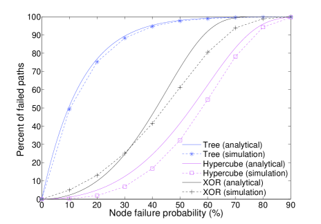
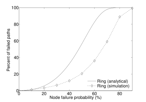
Figure 6: Both plots show the percentage of failed paths (i.e. 1-routability) for varying node failure probability and system size of N=$2^{16}$. (a) Analysis vs simulation: The simulation data points are reproduced from [2]. For all three routing geometries, the analytical curves show a great fit to the simulation curves. (b) Analysis vs simulation (ring): For the ring routing algorithm, the discrepancy between the analytical and simulation curve is due to the algorithm’s property that suboptimal hops contribute non-trivially to the routing process. In effect, the analytical curve provides an upper bound for percentage of failed paths. Note that the analytical curve is very close to simulation in the region of practical interest (i.e. for failure probability less than 20%)

.

4.3 Summary of Results for other Routing Geometries

Using the RCM method, the analytical expressions for the other DHT routing geometries can be similarly derived as for the hypercube routing geometry. In all the derivations, the majority of the work involves finding the expression for $p(h,q)$ through Markov chain modeling. Note that the analytical expressions derived in this section are compared with the simulation results obtained by Gummadi et al. [2] in Fig. 6 and 6.

For ease of exposition, we will use the notation $G(i,j)$, which denotes the probability that, starting at state $i$, the Markov chain ever visits state $j$. By any of the Markov chain models for the routing protocols, we note that $G(S_{0},S_{1})=1-Q(h)$, $G(S_{1},S_{2})=1-Q(h-1)$, and so forth, where the function $Q(m)$ can be thought of as the probability of failure at the $m$th phase of the routing process. As a result, all of the DHT systems under study have the property that the probability of successfully traveling $h$ hops or phases from the root node, $p(h,q)$, is given by the following common form:

$$p(h,q) = G(S_{0},S_{1})G(S_{1},S_{2})...G(S_{h-1},S_{h})$$ (5)

$$= \prod^{\small h}_{\small m=1}(1-Q(m))$$

Using Eq. 3, we see that only the expressions for $n(h)$ and $Q(m)$ are needed to compute the routability of the DHT routing system under investigation. As a result, we will only provide the $n(h)$ and $Q(m)$ expressions for each system for conciseness.

4.3.1 Tree

For the tree routing geometry, the routing distance distribution, $n(h)$, is $\binom{d}{h}$ by inspection. Furthermore, it is simple to show that $p(h,q)=(1-q)^{h}$ by examining the Markov chain model (see Fig. 4(a)). In sum, the expression for routability can be succinctly given as follows: $r=\frac{(2-q)^{d}-1}{(1-q)2^{d}-1}$

4.3.2 XOR

As reviewed in section 3, connecting to a neighbor at an XOR distance of $[2^{d-i},2^{d-i+1}]$ is equivalent to choosing a neighbor by matching the first (i-1) bits of one’s identifier, flipping the $i$th bit, and choose random bits for the rest of the bits. Note that this is equivalent to how neighbors are chosen in the Plaxton-tree routing geometry. As a result, the $n(h)$ expression is given as: $n(h)=\binom{n}{h}$ just as in the tree case.

Now, let’s examine how the Markov chain model (Fig. 5(b)) is obtained: in this scenario, a message is to be routed to a destination $h$ phases away; starting at state $S_{0}$, state $S_{1}$ is reached if the optimal neighbor correcting the leftmost bit exists, which happens with probability $1-q$ ($S_{i}$ denotes the state that corresponds to the $i$th advanced phase). However, if all $h$ neighbors have failed (i.e. with probability $q^{h}$), the failure state $F$ is entered. Otherwise, the routing process can correct one of the lower order bits, which happens with probability $q(1-q^{h-1})$. Note that there is a maximum number of $h-1$ lower order bits that can be corrected in the first phase. All other transition probabilities can be obtained similarly. By inspecting the Markov chain model, we note that $G(S_{0},S_{1})=1-Q_{xor}(h)$, $G(S_{1},S_{2})=1-Q_{xor}(h-1)$, and so forth, where the function $Q_{xor}(m)$ is defined as follows:

$$Q_{xor}(m) = q^{m}+\sum_{k=1}^{m-1}q^{m}[\displaystyle\prod^{m-1}_{j=m-k}(1-q^{j})]$$

$$\approx q^{m}(m+\frac{q}{1-q}(q^{m-1}(m-1)-\frac{1-q^{m+1}}{1-q}))$$

The approximation is obtained by invoking the following: $1-x\approx e^{-x}$ for x small.

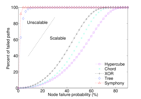
(a) System Size N=$2^{100}$

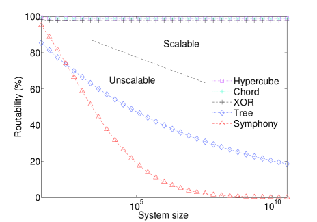
(b) Failure Probability q=0.1

Figure 7: (a) Asymptotic limit: This figure plots the percentage of failed paths (i.e. 1-routability) for varying node failure probability in the asymptotic limit. The curves are obtained by evaluating the analytical expressions at N=$2^{100}$. Note that the curves for tree and symphony are very close to a step function, which is consistent with our analysis. In addition, the curves for the other three geometries are very close to the case for N=$2^{16}$. (b) Routability vs N: This plot shows the routability of the routing geometries for varying system size and a constant failure probability (q=0.1). This figure clearly demonstrates the lack of scalability of the tree and Symphony routing geometries. As the system scales, the routability of both the tree and Symphony routing systems monotonically degrades toward zero. In contrast, the other three geometries remain highly routable in the face of failure even as the systems scale to billions of nodes. (In both plots, we set the number of near neighbors and the number of shortcuts equal to one for Symphony.)

4.3.3 Ring

In ring routing as implemented in Chord, when a node takes a suboptimal hop in the routing process, the progress made by taking this suboptimal hop is preserved in later hops. For example, consider the scenario that a message is to be routed to a node at a numeric distance that is $O(N)$ (i.e. the message is to be routed one full circle around the ring), and the fingers are connected to nodes that are half way across the ring, one quarter across the ring, etc. For the message’s first hop, it takes a suboptimal hop which takes the message only one quarter across the ring, because the finger that would have taken the message half way across the ring has failed. Then, for the message’s second hop, none of the finger connections has failed. Thus, the message takes an optimal hop which takes the message half way across the ring. Therefore, after two hops, the message is now three quarters of the way across the ring. Note that the progress made in the first suboptimal hop is this scenario is later preserved by a subsequent hop.

This property that suboptimal hops in ring routing contribute non-trivially to the routing process is not accounted for in the the Markov chain model as illustrated in Fig. 8(a). The reason is that accounting for progress made by suboptimal hops would lead to an exponential blowup in the number of terms that we need to keep track of for computing $p(h,q)$. This simplified Markov chain model essentially makes the assumption that progress made by suboptimal hops do not contribute to the routing process. Therefore, the analytical expression for $p(h,q)$ using this model provides a lower bound.

The Markov chain model for ring routing 8(a) is very similar to the one for XOR routing (Fig. 5(b)). However, fundamental differences exist: first, when a suboptimal hop is taken in Chord, the number of next hop choices does not decrease. For example, in the first phase, there are $h$ choices for the next hop, thus the transition probabilities from the states in the first phase to the failure state are given by $q^{h}$. In contrast, the corresponding transition probabilities in Fig. 5(b) are given by $q^{h}$, $q^{h-1}$, and so forth. In addition, the maximum number of suboptimal hops in Chord is given by $2^{h-1}$, $2^{h-2}$ and so forth, while the corresponding transition probabilities in Fig. 5(b) are given by $h$, $h-1$, and so forth. This difference is due to the fact that in XOR routing, routing fails if all the lower order bits are resolved and the leftmost bit is not yet resolved. However, Chord does not have such restriction.The results for the ring routing geometry is derived by inspecting Fig. 8(a):

$$Q_{ring}(m) =q^{m}\sum_{k=0}^{2^{m-1}-1}[q(1-q^{m-1})]^{k}$$

$$=q^{m}\frac{1-[q(1-q^{m-1})]^{2^{m-1}}}{1-q(1-q^{m-1})}$$

In addition, one can easily see by inspection that the $n(h)$ expression for the ring geometry is given by: $n(h)=2^{h-1}$.

4.3.4 Symphony

Symphony’s Markov chain model (Fig. 8(b)) is fundamentally different from the ones for XOR routing (Fig. 5(b)) and ring routing (Fig. 8(a)). Starting at $S_{0}$, one phase is advanced if any of the node’s shortcuts connects to the desired phase, which happens with probability $\frac{k_{s}}{d}$ where $k_{s}$ denotes the number of shortcuts. Alternatively, the routing fails if all of the node’s near neighbor and shortcut connections fail, which happens with probability $q^{k_{n}+k_{s}}$. The third possibility is taking a suboptimal hop, which happens with probability $1-\frac{k_{s}}{d}-q^{k_{n}+k_{s}}$. All other transition probabilities in the Markov chain can be similarly derived. Note that we approximate the maximum number of suboptimal hops by $\lceil\frac{d}{1-q}\rceil$.

For the Symphony routing geometry, we note that the expression for the $Q$’s is constant for all phases. The results are similarly derived as the other systems by inspecting Fig. 8(b):

$$Q_{sym} =q^{k_{n}+k_{s}}\sum^{\lceil\frac{d}{1-q}\rceil}_{j=0}(1-\frac{k_{s}}{d}-q^{k_{n}+k_{s}})^{j}$$

$$\approx q^{k_{n}+k_{s}}(\frac{1-(1-\frac{k_{s}}{d}-q^{k_{n}+k_{s}})^{\frac{d}{1-q}+1}}{1-(1-\frac{k_{s}}{d}-q^{k_{n}+k_{s}})})$$ (7)

The symbols $k_{n}$ and $k_{s}$ denote the number of near neighbors and shortcuts respectively. Similarly to ring routing, the $n(h)$ expression for the Symphony routing algorithm is given by: $n(h)=2^{h-1}$.

5 Scalability of DHT Routing Protocols under Random Failure

(a) Markov chain model for ring routing

(b) Markov chain model for Symphony routing

Figure 8: The above two diagrams illustrate the Markov chain model for ring and Symphony routing geometries.

For a DHT routing system to be scalable, its routability must converge to a non-zero value as the system size goes to infinity (Definition 2). Alternatively, we examine the asymptotic behavior of $p(h,q)$ with $h$ set to the average routing distance in the system (i.e. $h=O(\log N)$ or $O(\log^{2}N)$ for Symphony). Using Eq. 3, it is simple to show that the equivalent condition for scalability is as follows:

$$\lim_{N\rightarrow\infty}p(h,q)=\lim_{h\rightarrow\infty}p(h,q)>0\ \mbox{for}\ 0<q<1-p_{c}$$ (8)

Otherwise, the routing system is unscalable. In other words, the equivalent condition for system scalability states that as the number of routing hops to reach a destination node in the system approaches infinity, the probability of successfully routing to the destination node must not drop to zero for a non-zero node failure probability in the system.

As discussed in section 4.3, all of the DHT systems under study have the property that the probability of successfully traveling $h$ hops or phases from the root node is given by the following form:

$$p(h,q)=\prod^{h}_{m=1}(1-Q(m))$$ (9)

where $Q(m)$ can be thought of as the probability of failure at the $m$th phase of the routing process.

Theorem 1

(From Knopp [4]) If, for every $n$, $0\leq a_{n}<1$, then the product $\prod(1-a_{n})$ tends to a limit greater than 0 if, and only if, $\sum a_{n}$ converges.

Theorem 1 allows us to conveniently convert our problem of determining the convergence of an infinite product to a simpler infinite sum. Thus, $p(h,q)$ is convergent if and only if $\sum Q(m)$ converges.

5.1 Tree

The case for the tree routing geometry can be trivially shown to be unscalable:

$$\lim_{h\rightarrow\infty}(1-q)^{h}=0\ \ \mbox{for}\ \mbox{any}\ q>0$$ (10)

5.2 Hypercube

For hypercube routing, $p(h,q)$ is given by $p(h,q)=\displaystyle\prod^{h}_{m=1}(1-q^{m})$ (Eq. 2). By invoking Theorem 1, it is trivial to see that $\sum q^{m}$ converges for $0<q<1-p_{c}$. Thus, the hypercube routing geometry is scalable.

5.3 XOR

In XOR routing, the $Q(m)$ expression given by Eq. 4.3.2. It is simple to show that the $Q(m)$ series involves only $q^{m}$ and $mq^{m}$ terms. Thus, $\sum Q(m)$ is convergent and the XOR routing scheme is scalable.

5.4 Ring

We will demonstrate that the ring routing geometry is also scalable by showing that the XOR results derived above is a lower bound for the ring geometry. We compare the Markov chain models for the ring geometry and the XOR geometry (Fig. 8(a) and Fig. 5(b)). We note that the transition probabilities for the suboptimal hops in ring are strictly greater than the corresponding probabilities for XOR. For example, in Fig. 8(a), note that the transition probabilities for $S_{0}\rightarrow(0,1)$, $(0,1)\rightarrow(0,2)$ and so forth are given by $q(1-q^{h-1})$. These probabilities are strictly greater than the corresponding transition probabilities in Fig. 5(b). Thus, by comparing these two Markov chain models, it is simple to show that the $p(h,q)$ expression for the ring routing geometry is strictly greater than the $p(h,q)$ expression for XOR routing. Thus, the ring routing geometry is also scalable.

5.5 Symphony

In Symphony routing, the $Q(m)$ expression given by Eq. 7. Note that the $Q(m)$ expression is given by a constant term. Therefore, $\sum Q(m)$ is divergent and the Symphony routing scheme is unscalable.

Please refer to Fig. 7(a) and 7(b) for plots of the above scalability results.

6 Concluding Remarks

In this work, we present the reachable component method (RCM) which is an analytical framework for characterizing DHT system performance under random failures. The method’s efficacy is demonstrated through an analysis of five important existing DHT systems and the good agreement of the RCM predictions for each system with simulation results from the literature. Researchers involved in P2P system design and implementation can use the method to assess the performance of proposed architectures and to choose robust routing algorithms for application development. In addition, although the analysis presented in this work assumes fully-populated identifier spaces, analytical results for real world DHTs with non-fully-populated identifier spaces can be similarly derived. Detail investigation in this area will be left for future work.

One of the most interesting implications of this analysis is that in the large-network limit, some DHT routing systems are incapable of routing to a constant fraction of the network if there is any non-zero probability of random node failure. These DHT algorithms are therefore considered to be unscalable. Other algorithms are more robust to random node failures, allowing each node to route to a constant fraction of the network even as the system size goes to infinity. These systems are considered to be scalable. Now that real DHT implementations have on the order of millions of highly transient nodes, it is increasingly important to characterize how the size and failure conditions of a DHT will affect its routing performance.

7 Acknowledgments

We would like to thank Krishna Gummadi for furnishing the simulation results for DHT systems. We wish to thank Nikolaos Kontorinis for his feedback and suggestions. This work was in part supported by the NSF grants ITR:ECF0300635 and BIC:EMT0524843.

References

- [1] O. Angel, I. Benjamini, E. Ofek, and U. Wieder. Routing complexity of faulty networks. In Proceedings of PODC ’05, pages 209–217, New York, NY, USA, 2005. ACM Press.
- [2] K. Gummadi, R. Gummadi, S. Gribble, S. Ratnasamy, S. Shenker, and I. Stoica. The impact of dht routing geometry on resilience and proximity. In Proceedings of SIGCOMM ’03, pages 381–394, New York, NY, USA, 2003. ACM Press.
- [3] J. Kleinberg. The Small-World Phenomenon: An Algorithmic Perspective. In Proceedings of the 32nd ACM Symposium on Theory of Computing, 2000.
- [4] K. Knopp. Theory and Application of Infinite Series. Dover Publications, New York, 1990. Republication of the second English edition, 1951.
- [5] S. Krishnamurthy, S. El-Ansary, E. Aurell, and S. Haridi. A statistical theory of chord under churn. In 4th International Workshop on Peer-To-Peer Systems, Ithaca, New York, USA, February 2005.
- [6] S. S. Lam and H. Liu. Failure recovery for structured p2p networks: protocol design and performance evaluation. SIGMETRICS Perform. Eval. Rev., 32(1):199–210, 2004.
- [7] J. Li, J. Stribling, R. Morris, M. F. Kaashoek, and T. M. Gil. A performance vs. cost framework for evaluating dht design tradeoffs under churn. In Proceedings of the 24th Infocom, Miami, Florida, USA, March 2005.
- [8] D. Liben-Nowell, H. Balakrishnan, and D. Karger. Analysis of the Evolution of Peer-to-Peer Systems. In 21st ACM Symposium on Principles of Distributed Computing (PODC), Monterey, CA, July 2002.
- [9] D. Loguinov, A. Kumar, V. Rai, and S. Ganesh. Graph-theoretic analysis of structured peer-to-peer systems: routing distances and fault resilience. In Proceedings of SIGCOMM ’03, pages 395–406, New York, NY, USA, 2003. ACM Press.
- [10] G. S. Manku, M. Bawa, and P. Raghavan. Symphony: Distributed hashing in a small world. Proc. 4th USENIX Symposium on Internet Technologies and Systems, pages 127–140, 2003.
- [11] P. Maymounkov and D. Mazières. Kademlia: A peer-to-peer information system based on the xor metric. In Proceedings of IPTPS ’01, pages 53–65, London, UK, 2002. Springer-Verlag.
- [12] A. Parker. Peer-to-peer in 2005. Technical report, CacheLogic, 2005.
- [13] C. G. Plaxton, R. Rajaraman, and A. W. Richa. Accessing nearby copies of replicated objects in a distributed environment. In Proceedings of SPAA ’97, pages 311–320, New York, NY, USA, 1997. ACM Press.
- [14] S. Ratnasamy, P. Francis, M. Handley, R. Karp, and S. Shenker. A scalable content addressable network. In Proceedings of ACM SIGCOMM 2001, 2001.
- [15] D. Stauffer and A. Aharony. Introduction to Percolation Theory. Taylor & Francis, 1991.
- [16] I. Stoica, R. Morris, D. Liben-Nowell, D. R. Karger, M. F. Kaashoek, F. Dabek, and H. Balakrishnan. Chord: a scalable peer-to-peer lookup protocol for internet applications. IEEE/ACM Trans. Netw., 11(1):17–32, 2003.
- [17] S. Wang, D. Xuan, and W. Zhao. Analyzing and enhancing the resilience of structured peer-to-peer systems. J. Parallel Distrib. Comput., 65(2):207–219, 2005.