On Reduced Complexity Soft-Output MIMO ML detection

Abstract

In multiple-input multiple-output (MIMO) fading channels maximum likelihood (ML) detection is desirable to achieve high performance, but its complexity grows exponentially with the spectral efficiency. The current state of the art in MIMO detection is list decoding and lattice decoding. This paper proposes a new class of lattice detectors that combines some of the principles of both list and lattice decoding, thus resulting in an efficient parallelizable implementation and near optimal soft-ouput ML performance. The novel detector is called layered orthogonal lattice detector (LORD), because it adopts a new lattice formulation and relies on a channel orthogonalization process. It should be noted that the algorithm achieves optimal hard-output ML performance in case of two transmit antennas. For two transmit antennas max-log bit soft-output information can be generated and for greater than two antennas approximate max-log detection is achieved. Simulation results show that LORD, in MIMO system employing orthogonal frequency division multiplexing (OFDM) and bit interleaved coded modulation (BICM) is able to achieve very high signal-to-noise ratio (SNR) gains compared to practical soft-output detectors such as minimum-mean square error (MMSE), in either linear or nonlinear iterative scheme. Besides, the performance comparison with hard-output decoded algebraic space time codes shows the fundamental importance of soft-output generation capability for practical wireless applications.

I Introduction

Wireless transmission through multiple antennas, also referred to as multiple-input multiple-output (MIMO) radio, is currently enjoying a great popularity as it is considered the technology able to satisfy the ever increasing demand of high data rate communications. In MIMO fading channels and in presence of additive white Gaussian noise (AWGN), maximum-likelihood (ML) detection is optimal [1]. A straightforward implementation of the ML detector would require, for an uncoded complex constellation of size S and $L_{t}$ transmit antennas, an exhaustive search over all possible $S^{L_{t}}$ transmit sequences, thus being prohibitively complex for high spectral efficiencies. This observation justifies the intense interest in reduced complexity, sub-optimal linear detectors like zero-forcing (ZF) or minimum mean square error (MMSE) [2]. These algorithms currently represent the practical state-of-the-art for MIMO coded systems, as they can easily generate bit soft output information for use with powerful coded modulations. It should be noted that ZF and MMSE with spatial multiplexing offer diversity of $L_{r}-L_{t}+1$, where $L_{r}$ is the number of receive antennas, while optimum detection provides $L_{r}$ [3]; thus, linear detectors are highly suboptimal. Nonlinear detectors based on the combination of linear detectors and spatially ordered decision-feedback equalization (O-DFE) were proposed for V-BLAST in [4],[5]; they offer some performance improvement, but suffer noise enhancements due to nulling and error propagation due to interference cancellation (IC). More interesting for bit interleaved coded modulation (BICM) systems are soft-output iterative MMSE and error correction decoding strategies, in either ”hard” IC (HIC) [6] and soft IC (SIC) [7], [8] schemes. However they suffer from latency and complexity disadvantages.

To our knowledge, the class of ML approaching algorithms is quite limited. Two important families are the list-based detectors [9],[10],[11],[12],[13], based on the combination of ML and DFE principles, and the lattice decoders, among those the sphere decoder (SD) [14] is most well known.

The common idea of the list-based detectors (LD) is to divide the streams to be detected into two groups: first, one or more reference transmit streams are selected and a corresponding list of candidate constellation symbols is determined; then, for each sequence in the list, interference is cancelled from the received signal and the remaining symbol estimates are determined by as many sub-detectors operating on reduced size sub-channels. The IC process is analogous to V-BLAST spatial DFE; the differences lie in the criterion adopted to select the reference layer(s) and to order the remaining ones, and in the fact that its initial symbol estimate is replaced by a list of candidates. If the list includes all possible constellation points [9],[10], an initial stage of interference nulling is not required; this interference nulling is still performed if a reduced size sorted list is generated starting from the ZF estimates [11], [12]. The final hard-decision sequence is selected by minimizing the Euclidean distance (ED) metrics over the considered sequences. A particularly interesting result was obtained searching all possible S cases for a reference stream, or layer, and adopting O-DFE for the remaining $L_{t}-1$ sub-detectors. If a properly optimized layer ordering technique is utilized, numerical results reported in [10],[11] demonstrate that the LD detector is able to achieve full receive diversity and a degradation from ML performance of fractions of a dB. A notable property is that this can be accomplished through a parallel implementation, as the sub-detectors can operate independently. The drawback is that the computational complexity is high as $L_{t}$ O-DFE detectors for $L_{t}-1$ sub-streams have to be computed. If efficiently implemented [12], it involves $O(L_{t}^{4})$ complexity. Another major shortcoming of the prior work in list based detection is the absence of an algorithm to produce soft bit metrics for use in coding and decoding algorithms.

Lattice detectors use the linear nature of the MIMO channel to form a reduced complexity ML search. Lattice detectors are suitable for systems whose input-output relation can be represented as a real-domain linear model

$$\textbf{y}_{r}=\textbf{Bx}_{r}+\textbf{n}_{r}=\textbf{s}_{r}+\textbf{n}_{r}$$ (1)

where the information sequence $\textbf{x}_{r}$ is uniformly distributed over a discrete finite set $\mathcal{C}\subset R^{m}$, $\textbf{n}_{r}\in R^{n}$ represents the noise vector, B is a $n\times m$ real matrix where $n=2L_{r}$ and $m=2L_{t}$. The output signal vector $\textbf{s}_{r}\in\Lambda\subset{R^{n}}$. B represents the channel mapping of the transmit signals into the $m$-dimensional lattice $\Lambda$ and is also referred to as the lattice generator matrix. If the noise components are independent and identically distributed (i.i.d.) zero-mean Gaussian random variables (RVs) with a common variance, as typical of communication systems, then the ML decoding rule corresponds to solving the minimization problem:

$$\hat{\textbf{x}}_{r}=\arg\min_{\textbf{x}_{r}\in\,\mathcal{C}}\|\textbf{y}_{r}-\textbf{Bx}_{r}\|^{2}$$ (2)

where $\|\cdot\|$ denotes the vector norm. The problem in (2) is a constrained version of the closest vector problem (CVP) in lattice theory. A survey of closest point search methods has been presented in [15]. It should be noted that in the general case the model of (1) is still valid if a general encoder matrix $\textbf{G}\in R^{\,m\times m}$ is considered such that:

$$\textbf{x}_{r}=\textbf{Gu}_{r}$$ (3)

where $\textbf{u}_{r}\in\mathcal{U}\subset R^{m}$ is the information symbol sequence and $\textbf{x}_{r}$ is the transmit codeword. In this case the lattice generator matrix becomes BG. In the rest of the paper we will refer to (1) with no loss of generality. The lattice formulation for MIMO wireless systems was described in [16] in case of quadrature amplitude modulation (QAM) digitally modulated transmitted symbols.

SD can attain ML performance with significantly reduced complexity. Some efficient variants of the algorithm are summarized in [17]. SD presents a number of disadvantages, which can be summarized as follows:

• As the in-phase (I) and quadrature-phase (Q) components of the digitally modulated QAM symbols are searched in a serial fashion, SD is is not suitable for a parallel VLSI implementation. As a support to our claim, some papers have described the SD operations in terms of tree search and recently, the equivalence between the SD and the sequential decoder has been established rigorously [18].

• The number of lattice points to be searched is a random variable, sensitive to the channel and noise realizations, and to the initial radius. This implies a non-deterministic complexity and latency, not desirable for real-time high-data rate applications. Further, SD complexity has often been referred to as polynomial but a recent work [19] shows that SD remains an efficient solution only for problems of moderate size, and for SNR values in given ranges. This motivated the proposal of additional optional front-end processing to expedite the lattice search. However, lattice reduction (LR) techniques such as the Lenstra-Lenstra-Lovász [20], [21], [15] did not prove very useful to solve the constrained ML problem (2), as reported in [17], because they distort the original lattice and boundary control becomes difficult. These lattice reduction techniques are useful in conjunction with additional processing stage, i.e. the MMSE “generalized decision feedback equalizer” (MMSE-GDFE) [18]. When channel is slowly varying, these front-end processings are very effective on reducing the overall complexity. However, if channel changes significantly from block to block, front-end processings can have a significant impact on the overall complexity.

• Generation of soft output metrics is not easy with known lattice decoding algorithms. A solution was proposed in [22] and successively refined in [23], where bit log-likelihood ratios (LLR) are computed based on a ”candidate list” of sequences. No simple rule to determine the optimal size of such list was proposed; simulation results show that it can be very high (thousands of lattice points). This may nullify the benefits of using SD, in terms of complexity, as also evidenced in [24]. This observation is one of the main motivations of this work. Also, in case of use of LR techniques the problem of soft-output generation becomes prohibitively complex.

It should be noted that nulling and cancelling or equivalently ZF-DFE, besides being the core of the O-DFE algorithm [5], is also an important part of the SD operations. ZF-DFE can be efficiently implemented through a QR decomposition (QRD) of the channel matrix, as shown in [25],[9] and [17] for O-DFE and SD respectively.

In an attempt to retain the advantages of LD and SD algorithms at the same time addressing their main drawbacks, a novel MIMO lattice detector is proposed in this paper. This algorithm is given the name layered orthogonal lattice detector (LORD) [26],[27].

Similarly to SD, LORD consists of three different stages. First, the system is represented through a proper lattice formulation but different than the only one proposed for SD [16]. Second an efficient preprocessing of the channel matrix is implemented for ZF-DFE. While a standard QRD could be employed without altering the performance of the detection algorithm, a more computationally efficient Gram-Schmidt orthogonalization (GSO) process is outlined in this work. The last stage is the lattice search, which involves finding a proper subset of transmit sequences to solve the problem (2). The number of lattice points to be searched is linear in the number of transmit antennas and is easily modified to provide soft output bit metrics. The innovative concepts compared to SD, and already embedded in LD [10], is that the search of the lattice points can be accomplished in a parallel fashion, and their number is fully deterministic. LORD achieves a huge complexity reduction over the exhaustive-search ML algorithm and, as proven via numerical results, also obtains a better complexity-performance tradeoff than SD.

The proposed GSO technique avoids computing a complete QRD multiple times if the channel columns are permuted, as clear from the sequel. Compared to the best performing and efficiently implemented LD (”B-Chase” detector [12]) that relies on multiple QRDs, LORD algorithms has the following advantages. Its preprocessing is less complex - $O(L_{t}^{3})$ for $L_{t}=L_{r}$, instead of $O(L_{t}^{4})$); LORD generates reliable bit soft output information; it does not require any particular ordering scheme yet still retaining near-ML performance in BICM systems. Nevertheless, it should be noted that concepts like reduced complexity lattice search and optimal ordering schemes can be applied to LORD as well, with proper adaptations to real-domain; the explanation of these ideas is deferred to later works.

For two transmit antennas, LORD achieves ML hard-output demodulation and is able to compute optimal (max-log) bit LLRs. For more than two transmit antennas, the algorithm is suboptimal but still near-ML in BICM systems and its gain over MMSE-based linear and iterative nonlinear detectors actually increases with the dimensionality of the problem, thanks to a good exploitation of receive diversity. As shown later in this paper, even one single stage of LORD processing performs better than several iterations of MMSE-SIC in various orthogonal frequency division multiplexing (OFDM) BICM systems, with clear latency advantages. Iterative decoding and LORD detection schemes represent a promising topic for future work. Overall, these results suggest that soft-output MIMO near-ML detection, so far considered as computationally intractable for real-time high-data rate applications, can become a viable technique for next generation wireless communication systems.

To conclude this section, it should be mentioned that no efficient soft-output ML decoding strategy has been proposed so far for full diversity full data rate algebraic space-time codes (STCs) like the Golden Codes (GC) [28]. The performance comparison of layered BICM systems and uncoded GC provided in Section V shows that soft-output ML detection and ECCs are essential in order to exploit the high-data rate and high link robustness promised by MIMO for next generation wireless applications (like wireless local area networks (WLANs), undergoing standardization as IEEE 802.11n [29]).

The rest of the paper is organized as follows. In Section II the system notation and the novel lattice formulation are introduced. Section III is concerned with the description of the stages of LORD for two transmit antennas because LORD is optimal in this case. In Section III-A an efficient preprocessing algorithm is described; Section III-B focuses on the lattice search, and III-C deals with the bit soft output generation. Section IV and its subsections include a formulation of LORD suitable for any number of transmit antennas. Section V confirms through numerical results that LORD provides an excellent performance-complexity tradeoff. Finally, some concluding remarks are reported in Section VI.

II System Model and Lattice Representation

We consider a MIMO communication system with $L_{t}$ transmit and $L_{r}$ receive antennas, and a frequency nonselective fading channel. We also assume the receiver has perfect knowledge of the channel state and each receive antenna has a matched filter to the pulse shape. Then the complex baseband received signal $\textbf{y}_{c}=(Y_{c1}\,\ldots Y_{cL_{r}})^{T}$ is given by:

$$\textbf{y}_{c}=\sqrt{\frac{E_{s}}{L_{t}}}\,\textbf{H}_{c}\textbf{x}_{c}+\textbf{n}_{c}$$ (4)

where the input signal $\textbf{x}_{c}=(X_{c1}\,\ldots X_{cL_{t}})^{T}$ is the QAM or phase shift keying (PSK) complex information symbol vector, $E_{s}$ is the energy per transmitted symbol (under the hypothesis that the average constellation energy is $E[|X_{cj}|^{2}]=1$), n $=(N_{c1}\,\ldots N_{cL_{r}})^{T}$ is the $L_{r}\times 1$ complex white Gaussian noise (AWGN) sample vector, $\textbf{H}_{c}$ is the $L_{r}\times L_{t}$ complex channel matrix. The entries of $\textbf{H}_{c}$ are the i.i.d. complex path gains $H_{c\,ji}\sim\mathcal{N}_{c}(0,1)$ from transmit antenna $i$ to receive antenna $j$. At receive antenna $j$, the corrupting i.i.d. noise samples are $N_{cj}\sim\mathcal{N}_{c}(0,N_{0})$. As it will prove useful in the following, the $i^{th}$ column of $\textbf{H}_{c}$ is denoted as $\textbf{h}_{ci}$. Equation (4) is assumed to be valid per each OFDM tone if a MIMO-OFDM system and frequency selective channels are considered.

This paper assumes QAM modulation and derives a real lattice formulation. As a variant to the traditional lattice formulation [16], the system (4) can be translated into the form (1) performing appropriate scaling and ordering the I and Q of the complex entries as follows:

$$\textbf{x}_{r} = \left[X_{1,I},\ X_{1,Q},\ldots\,X_{L_{t},I},\ X_{L_{t},Q}\right]^{T}$$ (5)

$$= \left[x_{1},\ldots\,x_{2L_{t}}\right]^{T}$$

$$\textbf{y}_{r} = \left[Y_{1,I},\ Y_{1,Q},\ldots\,Y_{L_{r},I},\ Y_{L_{r},Q}\right]^{T}$$ (6)

$$\textbf{n}_{r} = \left[N_{1,I},\ N_{1,Q},\ldots\,N_{L_{r},I},\ N_{L_{r},Q}\right]^{T}.$$ (7)

Then (4) can be re-written as:

$$\textbf{y}_{r}=\sqrt{\frac{E_{s}}{L_{t}}}\,\textbf{H}_{r}\textbf{x}_{r}+\textbf{n}_{r}=\sqrt{\frac{E_{s}}{L_{t}}}\,\left[\begin{array}[]{ccc}\textbf{h}_{1},\ldots,\,\textbf{h}_{2L_{t}}\end{array}\right]\,\textbf{x}_{r}+\textbf{n}_{r}.$$ (8)

Each pair of columns ($\textbf{h}_{2k-1},\ \textbf{h}_{2k}$), $k=\{1,\ldots L_{t}\}$ of the real channel matrix $\textbf{H}_{r}$ has the form:

$$\textbf{h}_{2k-1}=\left[\Re{\left[H_{1k}\right]},\,\Im{\left[H_{1k}\right]},\ldots,\,\Re{\left[H_{L_{r}k}\right]},\,\Im{\left[H_{L_{r}k}\right]}\right]^{T}$$ (9)

$$\textbf{h}_{2k}=\left[-\Im{\left[H_{1k}\right]},\,\Re{\left[H_{1k}\right]},\ldots,\,-\Im{\left[H_{L_{r}k}\right]},\,\Re{\left[H_{L_{r}k}\right]}\right]^{T}$$ (10)

As a direct consequence of this formulation, they are pairwise orthogonal, i.e.

$$\textbf{h}_{2k-1}^{T}\textbf{h}_{2k}=0$$

where $k=\{1,\ldots,L_{t}\}$. This property will prove to be essential for LORD simplified demodulation. Other useful relations are:

$$\left\|\textbf{h}_{2k-1}\right\|^{2} = \left\|\textbf{h}_{2k}\right\|^{2}$$ (11)

$$\textbf{h}_{2k-1}^{T}\textbf{h}_{2j-1} = \textbf{h}_{2k}^{T}\textbf{h}_{2j},\quad\textbf{h}_{2k-1}^{T}\textbf{h}_{2j}=-\textbf{h}_{2k}^{T}\textbf{h}_{2j-1}$$

where $k,j=\{1,\ldots,L_{t}\}$ and $k\neq j$.

III LORD Algorithm - case of two transmit antennas

This section is concerned with the derivation of LORD algorithm for the case of $L_{t}=2$ transmit antennas. The two transmit antenna case is called out separately because in this case LORD is optimal. After the system is represented in the real-domain through the novel I and Q ordering, the proposed lattice detection algorithm requires two additional stages: preprocessing and lattice search. The purpose of preprocessing is to turn the MIMO channel into an upper triangular system. The proposed transformation is a computationally efficient alternate to a QRD as the normalizations are performed after the channel orthogonalization is completed, although a standard QRD would not impair the demodulation and performance properties of the algorithm.

III-A The preprocessing algorithm

The channel matrix can be represented as

$${\bf H}_{r}={\bf Q}{\bf R}{\bf\Lambda}_{q}$$ (12)

for $L_{r}\geq 2$. To show this it is noted that an $2L_{t}\times 2L_{r}$ orthogonal matrix can be defined

$${\bf Q}=\left[\begin{array}[]{ccc}\textbf{h}_{1}\quad\textbf{h}_{2}\quad\textbf{q}_{3}\quad\textbf{q}_{4}\end{array}\right]$$ (13)

where

$$\textbf{q}_{3} = \|\textbf{h}_{1}\|^{2}\textbf{h}_{3}-(\textbf{h}_{1}^{T}\textbf{h}_{3})\textbf{h}_{1}-(\textbf{h}_{2}^{T}\textbf{h}_{3})\textbf{h}_{2}$$ (14)

$$\textbf{q}_{4} = \|\textbf{h}_{1}\|^{2}\textbf{h}_{4}-(\textbf{h}_{1}^{T}\textbf{h}_{4})\textbf{h}_{1}-(\textbf{h}_{2}^{T}\textbf{h}_{4})\textbf{h}_{2}.$$ (15)

Then, remembering (11) one has:

$${\bf Q}^{T}{\bf Q}=\mbox{diag}\left[\left\|\textbf{h}_{1}\right\|^{2},\left\|\textbf{h}_{1}\right\|^{2},\left\|\textbf{q}_{3}\right\|^{2},\left\|\textbf{q}_{3}\right\|^{2}\right].$$ (16)

It can also be written that

$$\left\|\textbf{q}_{3}\right\|^{2}=\left\|\textbf{h}_{1}\right\|^{2}\left(\left\|\textbf{h}_{3}\right\|^{2}\left\|\textbf{h}_{1}\right\|^{2}-\left(\textbf{h}_{1}^{T}\textbf{h}_{3}\right)^{2}-\left(\textbf{h}_{2}^{T}\textbf{h}_{3}\right)^{2}\right)=\left\|\textbf{h}_{1}\right\|^{2}r_{3}$$ (17)

where by definition

$$r_{3}=\left\|\textbf{h}_{3}\right\|^{2}\left\|\textbf{h}_{1}\right\|^{2}-\left(\textbf{h}_{1}^{T}\textbf{h}_{3}\right)^{2}-\left(\textbf{h}_{2}^{T}\textbf{h}_{3}\right)^{2}.$$ (18)

By defining the $2L_{t}\times 2L_{t}$ upper triangular matrix

$${\bf R}=\left[\begin{array}[]{cccc}1&0&\textbf{h}_{1}^{T}\textbf{h}_{3}&\textbf{h}_{1}^{T}\textbf{h}_{4}\\ 0&1&\textbf{h}_{2}^{T}\textbf{h}_{3}&\textbf{h}_{2}^{T}\textbf{h}_{4}\\ 0&0&1&0\\ 0&0&0&1\end{array}\right]$$ (19)

and the $2L_{t}\times 2L_{t}$ diagonal matrix

$${\bf\Lambda}_{q}=\mbox{diag}\left[1,1,\ \left\|\textbf{h}_{1}\right\|^{-2},\left\|\textbf{h}_{1}\right\|^{-2}\right]$$ (20)

the original real channel matrix can be decomposed as

$${\bf H}_{r}={\bf Q}{\bf R}{\bf\Lambda}_{q}.$$ (21)

The linear preprocessing proposed in this paper is given as

$$\tilde{\textbf{y}}_{r}={\bf Q}^{T}\textbf{y}_{r}$$ (22)

where all values of ${\bf Q}$ are simple functions of the known channel coefficients. The signal model after preprocessing is given as

$$\tilde{\textbf{y}}_{r}=\sqrt{\frac{E_{s}}{2}}\,{\bf\tilde{R}}\textbf{x}_{r}+{\bf Q}^{T}\textbf{n}_{r}=\sqrt{\frac{E_{s}}{2}}\,\tilde{{\bf R}}\textbf{x}_{r}+\tilde{\textbf{n}}_{r}$$ (23)

where

$$\tilde{{\bf R}}={\bf Q}^{T}{\bf Q}{\bf R}{\bf\Lambda}_{q}=\left[\begin{array}[]{cccc}\left\|\textbf{h}_{1}\right\|^{2}&0&\textbf{h}_{1}^{T}\textbf{h}_{3}&\textbf{h}_{1}^{T}\textbf{h}_{4}\\ 0&\left\|\textbf{h}_{1}\right\|^{2}&\textbf{h}_{2}^{T}\textbf{h}_{3}&\textbf{h}_{2}^{T}\textbf{h}_{4}\\ 0&0&r_{3}&0\\ 0&0&0&r_{3}\end{array}\right].$$ (24)

is in the desired upper triangular form for lattice demodulation algorithms. System (23) is the real-domain lattice system equation the detection algorithm LORD uses, and is in the form of (1). The noise vector in the triangular model still has independent components but the components have unequal variances, i.e.,

$${\bf R}_{\tilde{n}_{r}}=E\left[\tilde{\textbf{n}}_{r}\tilde{\textbf{n}}_{r}^{T}\right]=\frac{N_{0}}{2}\,\mbox{diag}\left[\left\|\textbf{h}_{1}\right\|^{2},\ \left\|\textbf{h}_{1}\right\|^{2},\ \left\|\textbf{h}_{1}\right\|^{2}r_{3},\ \left\|\textbf{h}_{1}\right\|^{2}r_{3}\right].$$ (25)

The advantageous characteristic of the model formulation is that $\tilde{R}_{12}=\tilde{R}_{34}=0$, i.e., each of the I and Q components of each transmitted signal are broken into orthogonal dimensions and can be searched in an independent fashion.

As a further observation, all parameters needed in this triangularized model are a function of eight variables. Four of the variables are functions of the channel only, i.e.,

$$\sigma^{2}_{1}=\left\|\textbf{h}_{1}\right\|^{2}\qquad\sigma^{2}_{2}=\left\|\textbf{h}_{3}\right\|^{2}\qquad s_{1}=\textbf{h}_{1}^{T}\textbf{h}_{3}\qquad s_{2}=\textbf{h}_{1}^{T}\textbf{h}_{4}.$$ (26)

and four are functions of the channel and the observations, i.e.,

$$V_{1}=\textbf{h}_{1}^{T}\textbf{y}_{r}\qquad V_{2}=\textbf{h}_{2}^{T}\textbf{y}_{r}\qquad V_{3}=\textbf{h}_{3}^{T}\textbf{y}_{r}\qquad V_{4}=\textbf{h}_{4}^{T}\textbf{y}_{r}.$$ (27)

Also, equalities (11) imply that the $2\times 2$ matrix in the upper right corner of ${\bf\tilde{R}}$ is a rotation matrix. Specifically the required results for the upper triangular formulation is

$$\tilde{\textbf{y}}_{r}=\left[\begin{array}[]{c}\tilde{y_{1}}\\ \tilde{y_{2}}\\ \tilde{y_{3}}\\ \tilde{y_{4}}\end{array}\right]=\left[\begin{array}[]{c}V_{1}\\ V_{2}\\ \sigma^{2}_{1}V_{3}-s_{1}V_{1}+s_{2}V_{2}\\ \sigma^{2}_{1}V_{4}-s_{2}V_{1}-s_{1}V_{2}\end{array}\right]\quad{\bf\tilde{R}}=\left[\begin{array}[]{cccc}\sigma^{2}_{1}&0&s_{1}&s_{2}\\ 0&\sigma^{2}_{1}&-s_{2}&s_{1}\\ 0&0&\sigma^{2}_{1}\sigma^{2}_{2}-s_{1}^{2}-s_{2}^{2}&0\\ 0&0&0&\sigma^{2}_{1}\sigma^{2}_{2}-s_{1}^{2}-s_{2}^{2}\end{array}\right].$$ (28)

This formulation results in a preprocessing complexity (expressed in terms of real multiplications, RMs) that is $O(16L_{r}+9)$.

As it will prove useful when dealing with soft output generation, we also notice that shifting the ordering of the transmit antennas results in a similar model:

$$\tilde{\textbf{y}}_{s}=\sqrt{\frac{E_{s}}{2}}\,\tilde{{\bf R}}_{s}\textbf{x}_{s}+\tilde{\textbf{n}}_{s}$$ (29)

where

$$\tilde{\textbf{y}}_{s}=\left[\begin{array}[]{c}\tilde{y_{s1}}\\ \tilde{y_{s2}}\\ \tilde{y_{s3}}\\ \tilde{y_{s4}}\end{array}\right]=\left[\begin{array}[]{c}V_{3}\\ V_{4}\\ \sigma^{2}_{2}V_{1}-s_{1}V_{3}-s_{2}V_{4}\\ \sigma^{2}_{2}V_{2}+s_{2}V_{3}-s_{1}V_{4}\end{array}\right]\,{\bf\tilde{R}}_{s}=\left[\begin{array}[]{cccc}\sigma^{2}_{2}&0&s_{1}&-s_{2}\\ 0&\sigma^{2}_{2}&s_{2}&s_{1}\\ 0&0&\sigma^{2}_{1}\sigma^{2}_{2}-s_{1}^{2}-s_{2}^{2}&0\\ 0&0&0&\sigma^{2}_{1}\sigma^{2}_{2}-s_{1}^{2}-s_{2}^{2}\end{array}\right]$$ (30)

$${\bf R}_{\tilde{n}_{s}}=E\left[\tilde{\textbf{n}}_{s}\tilde{\textbf{n}}_{s}^{T}\right]=\frac{N_{0}}{2}\,\mbox{diag}\left[\left\|\textbf{h}_{3}\right\|^{2},\ \left\|\textbf{h}_{3}\right\|^{2},\ \left\|\textbf{h}_{3}\right\|^{2}r_{3},\ \left\|\textbf{h}_{3}\right\|^{2}r_{3}\right]$$ (31)

and $\textbf{x}_{s}=\left[x_{3}\,x_{4}\,x_{1}\,x_{2}\right]^{T}$.

Finally, we observe that there is an interesting relationship between the triangularized model parameters and the complex channel coefficients. First it should be noted that $\sigma^{2}_{1}=\left|\textbf{h}_{c1}\right|^{2}$ and that $\sigma^{2}_{2}=\left|\textbf{h}_{c2}\right|^{2}$. Secondly, the sample cross correlation between the gains for transmit antenna 1 and transmit antenna 2 is given as

$$\textbf{h}_{c2}^{H}\textbf{h}_{c1}=s_{1}+js_{2}.$$ (32)

A sample crosscorrelation coefficient can be defined as

$$\rho_{12}=\frac{\textbf{h}_{c2}^{H}\textbf{h}_{c1}}{\sqrt{\sigma^{2}_{1}\sigma^{2}_{2}}}.$$ (33)

Using (33), formula (18) can be written as

$$r_{3}=\sigma^{2}_{1}\sigma^{2}_{2}\left(1-\left|\rho_{12}\right|^{2}\right).$$ (34)

It is apparent that when $L_{r}$ gets large the magnitude of $\rho_{12}$ will go to zero and the MIMO detection problem for each antenna will become completely decoupled.

III-B Lattice search and demodulation

The system equations defined in Section III-A lead naturally to a simplified yet optimal ML demodulation. Consider a PSK or QAM constellation of size S. The discussion in this paper will assume that $(M^{2})$-QAM modulation is used on each antenna but a generalization to any linear modulation is possible. The optimum ML word demodulator (2) would have to compute the ML metric for $M^{2L_{t}}$ constellation points and has a complexity $O(M^{4})$ for $L_{t}=2$.

The notation used in the sequel is that $\Omega_{x}$ will refer to the M-PAM constellation for each real dimension. Given the formulation in (23)-(28) and neglecting scalar energy normalization factors to simplify the notation, the ML decision metric becomes

$$T(\textbf{x}_{r}) = \left\|\tilde{\textbf{y}}_{r}-\tilde{\textbf{R}}\textbf{x}_{r}\right\|^{2}=\frac{\left(\tilde{y}_{1}-\sigma^{2}_{1}x_{1}-s_{1}x_{3}-s_{2}x_{4}\right)^{2}}{\sigma^{2}_{1}}+\frac{\left(\tilde{y}_{2}-\sigma^{2}_{1}x_{2}+s_{2}x_{3}-s_{1}x_{4}\right)^{2}}{\sigma^{2}_{1}}$$ (35)

$$+\frac{\left(\tilde{y}_{3}-r_{3}x_{3}\right)^{2}}{\sigma^{2}_{1}r_{3}}+\frac{\left(\tilde{y}_{4}-r_{3}x_{4}\right)^{2}}{\sigma^{2}_{1}r_{3}}$$

The ML demodulator finds the maximum value of the metric over all possible values of the sequence $\textbf{x}_{r}$. This search can be greatly simplified by noting for given values of $x_{3}$ and $x_{4}$ the maximum likelihood metric reduces to

$$T(\textbf{x}_{r})=\frac{\left(\tilde{y}_{1}-\sigma^{2}_{1}x_{1}-C_{1}(x_{3},x_{4})\right)^{2}}{\sigma^{2}_{1}}+\frac{\left(\tilde{y}_{2}-\sigma^{2}_{1}x_{2}-C_{2}(x_{3},x_{4})\right)^{2}}{\sigma^{2}_{1}}+C_{3}(x_{3},x_{4})$$ (36)

where

$$C_{1}(x_{3},x_{4})=s_{1}x_{3}+s_{2}x_{4}\qquad C_{2}(x_{3},x_{4})=-s_{2}x_{3}+s_{1}x_{4}\qquad C_{3}(x_{3},x_{4})\geq 0$$ (37)

The originality of LORD stems from the fact that - as clear from (36) - the conditional ML decision on $x_{1}$ and $x_{2}$ can immediately be made by a simple threshold test, i.e.,

$$\hat{x}_{1}(x_{3},x_{4})=\mbox{round}\left(\frac{\tilde{y}_{1}-C_{1}(x_{3},x_{4})}{\sigma^{2}_{1}}\right),\quad\hat{x}_{2}(x_{3},x_{4})=\mbox{round}\left(\frac{\tilde{y}_{2}-C_{2}(x_{3},x_{4})}{\sigma^{2}_{1}}\right).$$ (38)

where the round operation is a simple slicing operation to the constellation elements of $\Omega_{x}$. This property is direct consequence of the orthogonality of the problem formulation. The final ML estimate is then given as

$$\left\{\hat{x}_{1}(\hat{x}_{3},\hat{x}_{4}),\hat{x}_{2}(\hat{x}_{3},\hat{x}_{4}),\hat{x}_{3},\hat{x}_{4}\right\}=\arg\stackrel{{\scriptstyle\textstyle\min}}{{\scriptstyle x_{3},x_{4}\in\Omega_{x}^{2}}}\left\{\frac{\left(\tilde{y}_{1}-\sigma^{2}_{1}\hat{x}_{1}(x_{3},x_{4})-C_{1}(x_{3},x_{4})\right)^{2}}{\sigma^{2}_{1}}\right.$$

$$+\left.\frac{\left(\tilde{y}_{2}-\sigma^{2}_{1}\hat{x}_{2}(x_{3},x_{4})-C_{2}(x_{3},x_{4})\right)^{2}}{\sigma^{2}_{1}}+C_{3}(x_{3},x_{4})\right\}$$ (39)

This implies that the number of points that has to be searched in this formulation to find the true ML estimator is $M^{2}$ (with two slicing operations per searched point). This is a significant saving in complexity.

It should be noticed that, in a direct analogy to (29)-(30), the ML estimate could as well be found minimizing the reordered ML decision metric

$$T^{\prime}(\textbf{x}_{s}) = \left\|\tilde{\textbf{y}}_{s}-\tilde{\textbf{R}}_{s}\textbf{x}_{s}\right\|^{2}=\frac{\left(\tilde{y}_{s1}-\sigma^{2}_{2}x_{3}-s_{1}x_{1}+s_{2}x_{2}\right)^{2}}{\sigma^{2}_{2}}+\frac{\left(\tilde{y}_{s2}-\sigma^{2}_{2}x_{4}-s_{2}x_{1}-s_{1}x_{2}\right)^{2}}{\sigma^{2}_{2}}$$ (40)

$$+\frac{\left(\tilde{y}_{s3}-r_{3}x_{1}\right)^{2}}{\sigma^{2}_{2}r_{3}}+\frac{\left(\tilde{y}_{s4}-r_{3}x_{2}\right)^{2}}{\sigma^{2}_{2}r_{3}}.$$

Similarly to (38)-(III-B), minimization of (40) can be accomplished considering all possible $M^{2}$ values for $(x_{1},x_{2})$ and obtaining the corresponding $\left(\hat{x}_{3}(x_{1},x_{2}),\hat{x}_{4}(x_{1},x_{2})\right)$ through rounding operations to the constellation elements of $\Omega_{x}$.

We observe that this reduced complexity ML demodulation is a direct consequence of the reordered lattice formulation. Each group of two rows in the model (28) corresponds to a transmit antenna, or layer (the two terms will be used interchangeably in the remainder of the paper). Equation (38) shows that the decisions for the top layer can be made independently for the I and the Q modulation. If the traditional lattice formulation [16] is adopted instead, in (35) the partial ED (PED) terms corresponding to the higher rows of the triangularized model become dependent on all the lower layers of the transmit modulation, and the simplified demodulation (III-B) is no longer possible.

Two further observations conclude this section:

-

The search of the lattice points can be carried out in a completely parallel fashion. This solves one of the drawbacks of SD algorithm, characterized by a recursive - i.e. serial - search, and is desirable for VLSI implementations.

-

The lattice point enumeration technique, i.e. method of spanning the points during the search, is not important for LORD as long as all $M^{2}$ possible cases for the bottom layer are searched. However, we observe that ordering the candidate list according to an increasing ED from the receiver observations has important implications for suboptimal searches, i.e. if less than $M^{2}$ values for the bottom layer are considered. This corresponds to the Schnorr-Euchner (SE) [21],[14] enumeration method. Future work will address this important sub-optimal and reduced-complexity version of LORD.

III-C LLR generation

This section deals with the reduced-complexity generation of reliable soft output information. This problem is often neglected in lattice decoding literature because of the intrinsic difficulties caused by the SD attempt to reduce to the minimum the number of searched lattice points. As mentioned in Section I, a partial solution to this issue has been proposed in [22], [23] with the introduction of the so-called ”candidate list”. Unfortunately the random nature of the selected points to be stored in this list pose several implementation and complexity issues, also evidenced in [24]. To name a few, no rule to optimally size the list has been proposed, and simulation results show that in order to obtain reliable LLRs the size depends on the considered MIMO scenario; also, points are stored in the list in an inherently sequential manner; the ”quality” of the points stored in the list, as well as the total number of searched sequences before the search can be declared concluded, strongly depends on choice of the sphere radius. The use of LR techniques can only help in making the convergence to the ML solution faster, but precludes the detection algorithm from computing soft-output values, because the boundaries of the information set are no more recognizable after the application of such techniques. The choice followed in this work was then to avoid LR methods and to solve the indeterministic and sequential nature of the selection of the sequences needed for the generation of reliable bit soft-output information.

The problem is first recalled for the complex-domain system (4). If $M^{2}$-QAM constellation is considered for the information symbol vector and $M_{c}$ is the number of bits per symbol, the LLR or logarithmic a-posteriori probability (APP) ratio of the bit $b_{k}$, $k=1,\ldots,2M_{c}\,$, conditioned on the received channel symbol vector $\textbf{y}_{c}$, is often expressed as:

$$L(b_{k}|\textbf{y}_{c})=\ln{\frac{P(b_{k}=1|\textbf{y}_{c})}{P(b_{k}=0|\textbf{y}_{c})}}=\ln{\frac{\displaystyle\sum_{{\bf x}_{c}\in S(k)^{+}}P(\textbf{y}_{c}|\textbf{x}_{c})P_{a}(\textbf{x}_{c})}{\displaystyle\sum_{{\bf x}_{c}\in S(k)^{-}}P(\textbf{y}_{c}|\textbf{x}_{c})P_{a}(\textbf{x}_{c})}}$$ (41)

In (41) $S(k)^{+}$ ($S(k)^{-}$) is the set of $2^{2Mc-1}$ bit sequences having $b_{k}=1$ ($b_{k}=0$); $P_{a}({\bf x}_{c})$ represents the a-priori probabilities of $\textbf{x}_{c}$ and will be neglected in the rest of this paper as equiprobable transmit symbols are considered. From (4), the likelihood function $\displaystyle P(\textbf{y}_{c}|\textbf{x}_{c})$ is given by:

$$P(\textbf{y}_{c}|\textbf{x}_{c})\propto\exp{\left[-\frac{1}{2\sigma^{2}}\|\textbf{y}_{c}-\sqrt{\frac{E_{s}}{2}}\textbf{Hx}_{c}\|^{2}\right]}=\exp{\left[-D(\textbf{x}_{c})\right]}$$ (42)

where $\sigma^{2}=N_{0}/2$ and $D(\textbf{x}_{c})$ is the ED term. The summation of exponentials involved in (41) can be approximated according to the following so-called max-log approximation:

$$\ln{\sum_{{\bf x}\in S(k)^{+}}\exp{\left[-D({\bf x})\right]}}\approx\ln{\max_{{\bf x}\in S(k)^{+}}{\exp{\left[-D({\bf x})\right]}}}=-\min_{{\bf x}\in S(k)^{+}}{D({\bf x})}$$ (43)

Expression (43) is equivalent to neglecting a correction term in the exact log-domain version of (41), which uses the “Jacobian logarithm” or $\max^{*}$ function

$$\textrm{jacln}(a,b):=\ln{\left[\exp{(a)}+\exp{(b)}\right]}=\max{(a,b)}+\ln{\left[1+\exp{(-|a-b|)}\right]}.$$ (44)

As shown e.g. in [30], the performance degradation caused by the max-log approximation is generally very small compared to the use of the $\max^{*}$ function. Using (43) in (41), max-log bit LLRs can then be written as:

$$L(b_{k}|\textbf{y}_{c})\approx\min_{{\bf x}_{c}\in S(k)^{-}}{D(\textbf{x}_{c})}-\min_{{\bf x}_{c}\in S(k)^{+}}{D(\textbf{x}_{c})}$$ (45)

Expression (45) involves two minimization problems, i.e. for each bit index $k=1,\ldots,2M_{c}\,$ it requires identification of the most likely transmit sequence (or lattice point) where $b_{k}=1$ and the most likely one where $b_{k}=0$. By definition, one of the two sequences is the hard-decision ML solution of (2). However, using SD, there is no guarantee that the other sequence is found during the lattice search. LORD does not have this problem, as shown in the sequel.

The formulation of the problem in case of real-domain lattice equations is perfectly similar. From (23) the LLRs assume the form:

$$L(b_{k}|\tilde{\textbf{y}}_{r})=\ln{\frac{\displaystyle\sum_{{\bf x}_{r}\in S(k)^{+}}P(\tilde{\textbf{y}}_{r}|\textbf{x}_{r})}{\displaystyle\sum_{{\bf x}_{r}\in S(k)^{-}}P(\tilde{\textbf{y}}_{r}|\textbf{x}_{r})}}$$ (46)

where, recalling (35), the likelihood function $\displaystyle P(\tilde{\textbf{y}}_{r}|\textbf{x}_{r})$ is given by:

$$P(\tilde{\textbf{y}}_{r}|\textbf{x}_{r})=\exp\left[-|T(\textbf{x}_{r})|\right].$$ (47)

Let us first focus on the bits corresponding to the complex symbol $X_{c2}$ in the symbol sequence $\textbf{x}_{c}=(X_{c1}\,\,X_{c2})^{T}$. By employing arguments similar to those that led to the simplified ML estimator (III-B), it can be easily proven that the two ED terms needed for every bit in $X_{c2}$ are certainly found computing (35) over the possible $M^{2}$ values of $X_{c2}=(x_{3},\,x_{4})$ and minimizing the expression over $X_{c1}=(x_{1},\,x_{2})$, for every value of $X_{c2}$. This last operation is simply carried out through the slicing operation to the constellation elements of $\Omega_{x}$, described in (38). The LLRs relative to the bits corresponding to $X_{2}$, $b_{2,k}$, can then be written as:

$$L(b_{2,k}|\tilde{\textbf{y}})\approx\min_{x_{3},x_{4}\in S(k)_{2}^{-}}{T(\textbf{x}_{r})}-\min_{x_{3},x_{4}\in S(k)_{2}^{+}}{T(\textbf{x}_{r})}$$ (48)

where $k=1,\ldots,M_{c}$, and $S(k)_{2}^{+}$ ($S(k)_{2}^{-}$) are the set of $2^{M_{c}-1}$ bit sequences having $b_{2,k}=1$ ($b_{2,k}=0$).

The computation of the LLRs for the bits corresponding to symbol $X_{1}$ can be obtain by a simple reordering of the model and a repeating of the LORD processing, as for (29)-(30). Recalling that $\textbf{x}_{s}=\left[x_{3}\,x_{4}\,x_{1}\,x_{2}\right]$ is the reordered information sequence, using (40) the LLRs of the bits corresponding to $X_{1}$, $b_{1,k}$, can be written as

$$L(b_{1,k}|\tilde{\textbf{y}_{s}})\approx\min_{x_{1},x_{2}\in S(k)_{1}^{-}}{T^{\prime}(\textbf{x}_{s})}-\min_{x_{1},x_{2}\in S(k)_{1}^{+}}{T^{\prime}(\textbf{x}_{s})}$$ (49)

where $k=1,\ldots,M_{c}$, $S(k)_{1}^{+}$ ($S(k)_{1}^{-}$) are the set of $2^{M_{c}-1}$ bit sequences having $b_{1,k}=1$ ($b_{1,k}=0$). There is significant complexity reduction that can be utilized in forming the LLR. By comparing (28) and (30), it is apparent that much of the preprocessing computation needed in (28) can be used in the reordered (30). The resulting complexity of the preprocessing stage will be $O(16L_{r}+12)$. The lattice search for both orderings will have complexity $O(2M^{2})$ due to the max-log LLR computation.

IV LORD Algorithm - case of $L_{t}$ transmit antennas

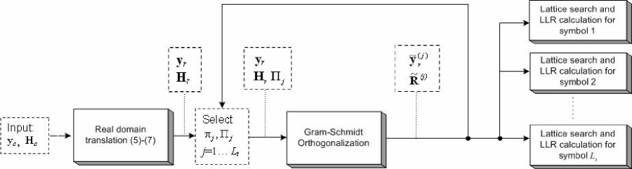
Figure 1: Block diagram of LORD detector.

The LORD detection algorithm can be generalized to any $L_{t}>2$ and $L_{r}\geq L_{t}$ in a sub-optimal way but still often remaining near-ML, as shown in Section V. Specifically, a computationally efficient QRD algorithm is described in Section IV-A. A notationally compact and elegant recursive variant of QRD is given in the Appendix. The relation between the extended and the compact representations is analogous to that existing between QRD through GSO and modified GSO (MGSO) [31]. The main difference between the GSO proposed in this paper and the QRD [31] is represented by the way the normalizations are handled, as clear from the sequel. The lattice search and soft output generation are then obtained generalizing the steps described in III-B and III-C respectively. A block diagram highlighting LORD algorithm steps is reported in Fig. 1.

IV-A The preprocessing algorithm - standard formulation

The formulation described in the sequel can be viewed as a generalization of the equations reported in Section III-A for $L_{t}=2$. This preprocessing corresponds to GSO with normalizations deferred to a later stage. To best understand this preprocessing note that there is an $2L_{t}\times 2L_{r}$ orthogonal matrix

$${\bf Q}=\left[\begin{array}[]{ccc}\textbf{q}_{1}\quad\textbf{q}_{2}\quad\textbf{q}_{3}\quad\textbf{q}_{4}\,\ldots\,\textbf{q}_{2L_{t}-1}\quad\textbf{q}_{2L_{t}}\end{array}\right].$$ (50)

where

$$\textbf{q}_{1} = \textbf{h}_{1}$$ (51)

$$\textbf{q}_{2} = \textbf{h}_{2}$$

$$\textbf{q}_{3} = \sigma_{1}^{2}\textbf{h}_{3}-s_{1,3}\textbf{h}_{1}-s_{2,3}\textbf{h}_{2}$$

$$\textbf{q}_{4} = \sigma_{1}^{2}\textbf{h}_{4}-s_{1,4}\textbf{h}_{1}-s_{2,4}\textbf{h}_{2}$$

$$\textbf{q}_{5} = r_{3}\sigma_{1}^{2}\textbf{h}_{5}-r_{3}s_{1,5}\textbf{h}_{1}-r_{3}s_{2,5}\textbf{h}_{2}-t_{3,5}\textbf{q}_{3}-t_{4,5}\textbf{q}_{4}$$ (52)

$$\vdots$$

$$\textbf{q}_{p} = P_{1}^{k}\left[\sigma_{1}^{2}\textbf{h}_{p}-s_{1,p}\textbf{h}_{1}-s_{2,p}\textbf{h}_{2}\right]-\sum_{i=2}^{k-1}\left[P_{i+1}^{k}\left(t_{2i-1,p}\textbf{q}_{2i-1}+t_{2i,p}\textbf{q}_{2i}\right)\right]-t_{2k-1,p}\textbf{q}_{2k-1}-t_{2k,p}\textbf{q}_{2k}$$

where $p$ denotes the generic $k-th$ pair of q columns, i.e. $p=\{2k+1,2k+2\}$, with $k=\{2,\ldots,L_{t}-1\}$, and which uses the following definitions:

$$s_{j,k}\equiv\textbf{h}_{j}^{T}\textbf{h}_{k},\qquad t_{j,k}\equiv\textbf{q}_{j}^{T}\textbf{h}_{k},\qquad\sigma_{k}^{2}\equiv\left\|h_{k}^{2}\right\|\qquad P_{m}^{n}\equiv\prod_{j=m}^{n}r_{2j-1}$$ (53)

where $m,n$ are integers with $1\leq m\leq n$. The terms $r_{2k-1}$, with $k=\{1,\ldots L_{t}\}$, are given by:

$$r_{1} = 1$$

$$\quad r_{3} = \quad\sigma_{3}^{2}\sigma_{1}^{2}-s_{1,3}^{2}-s_{2,3}^{2}$$ (54)

$$\vdots$$

$$r_{2k-1} = P_{2}^{k-1}\left(\sigma_{1}^{2}\sigma_{2k-1}^{2}-s_{1,2k-1}^{2}-s_{2,2k-1}^{2}\right)-\sum_{i=2}^{k-2}{P_{i+1}^{k-1}\left(t_{2i-1,2k-1}^{2}+t_{2i,2k-1}^{2}\right)}$$

$$-t_{2k-3,2k-1}^{2}-t_{2k-2,2k-1}^{2}.$$

They can also be written in the compact form

$$r_{2k-1}=P_{2}^{k-1}\sigma_{1}^{2}\sigma_{2k-1}^{2}(1-|\rho_{1,k}|^{2}-\sum_{i=2}^{k-1}|{\rho\prime}_{i,k}|^{2})$$ (56)

where we have used the square magnitudes of the (generalized) correlation coefficients:

$$|\rho_{k,j}|^{2} = \frac{s_{2k-1,2j-1}^{2}+s_{2k-1,2j}^{2}}{\sigma_{2k-1}^{2}\sigma_{2j-1}^{2}}$$ (57)

$$|{\rho\prime}_{k,j}|^{2} = \frac{t_{2k-1,2j-1}^{2}+t_{2k-1,2j}^{2}}{\left\|\textbf{q}_{2k-1}\right\|^{2}\sigma_{2j-1}^{2}},\,j>k.$$

It is easily shown that (11) can be generalized as:

$$\|\textbf{q}_{2k-1}\|^{2} = \|\textbf{q}_{2k}\|^{2}=P_{1}^{k}\sigma_{1}^{2}$$ (58)

$$\textbf{q}_{2k-1}^{T}\textbf{h}_{2j-1} = \textbf{q}_{2k}^{T}\textbf{h}_{2j},\qquad\textbf{q}_{2k-1}^{T}\textbf{h}_{2j}=-\textbf{q}_{2k}^{T}\textbf{h}_{2j-1},\,j>k.$$

Also, by construction the q vectors, and {q,h} couples, are pairwise orthogonal, i.e.

$$\textbf{q}_{2k-1}^{T}\textbf{q}_{2k}=0,\quad\textbf{q}_{2k-1}^{T}\textbf{h}_{2k}=0$$

The orthogonal matrix Q then satisfies

$${\bf Q}^{T}{\bf Q}=\mbox{diag}\left[\sigma_{1}^{2},\ \sigma_{1}^{2},\ \left\|\textbf{q}_{3}\right\|^{2},\ \left\|\textbf{q}_{3}\right\|^{2},\ldots,\ \left\|\textbf{q}_{2L_{t}-1}\right\|^{2},\ \left\|\textbf{q}_{2L_{t}-1}\right\|^{2}\right]$$ (59)

By defining the $2L_{t}\times 2L_{t}$ upper triangular matrix

$${\bf R}=\left[\begin{array}[]{cccccccccc}1&0&s_{1,3}&s_{1,4}&r_{3}s_{1,5}&\ldots&\ldots&\ldots&P^{L_{t}-1}_{1}s_{1,2L_{t}-1}&P^{L_{t}-1}_{1}s_{1,2L_{t}}\\ 0&1&-s_{1,4}&s_{1,3}&-r_{3}s_{1,6}&\ldots&\ldots&\ldots&-P^{L_{t}-1}_{1}s_{1,2L_{t}}&P^{L_{t}-1}_{1}s_{1,2L_{t}-1}\\ 0&0&1&0&t_{3,5}&\ldots&\ldots&\ldots&P^{L_{t}-1}_{2}t_{3,2L_{t}-1}&P^{L_{t}-1}_{2}t_{3,2L_{t}}\\ 0&0&0&1&t_{4,5}&\ldots&\ldots&\ldots&-P^{L_{t}-1}_{2}t_{3,2L_{t}}&P^{L_{t}-1}_{2}t_{3,2L_{t}-1}\\ \ldots&\ldots&\ldots&\ldots&\ldots&\ldots&\ldots&\ldots&\ldots&\ldots\\ 0&0&0&0&0&\ldots&1&0&t_{2L_{t}-3,2L_{t}-1}&t_{2L_{t}-3,2L_{t}}\\ 0&0&0&0&0&\ldots&0&1&-t_{2L_{t}-3,2L_{t}}&t_{2L_{t}-3,2L_{t}-1}\\ 0&0&0&0&0&\ldots&0&0&1&0\\ 0&0&0&0&0&\ldots&0&0&0&1\\ \end{array}\right]$$ (60)

the real channel matrix $\textbf{H}_{r}$ can be decomposed in the product:

$${\bf H}_{r}={\bf Q}{\bf R}{\bf\Lambda}_{q}$$ (61)

where the $2L_{t}\times 2L_{t}$ diagonal matrix

$${\bf\Lambda}_{q}=\mbox{diag}\left[1,1,\ \sigma_{1}^{-2},\sigma_{1}^{-2},\ldots\left(P_{1}^{L_{t}-1}\sigma_{1}^{2}\right)^{-1}\right]$$ (62)

includes the normalization factors due to the fact that Q is not orthonormal. Note again all values of ${\bf Q}$ are simple functions of the known channel coefficients. Again the signal model after preprocessing is given as

$$\tilde{\textbf{y}}_{r}=\sqrt{\frac{E_{s}}{2}}\,{\bf\tilde{R}}\textbf{x}_{r}+{\bf Q}^{T}\textbf{n}_{r}=\sqrt{\frac{E_{s}}{2}}\,\tilde{{\bf R}}\textbf{x}_{r}+\tilde{\textbf{n}}_{r}.$$ (63)

The triangular matrix $\tilde{{\bf R}}={\bf Q}^{T}{\bf Q}{\bf R}{\bf\Lambda}_{q}$, given by:

$$\tilde{{\bf R}}=\left[\begin{array}[]{cccccccccc}\sigma_{1}^{2}&0&s_{1,3}&s_{1,4}&s_{1,5}&\ldots&\ldots&\ldots&s_{1,2L_{t}-1}&s_{1,2L_{t}}\\ 0&\sigma_{1}^{2}&-s_{1,4}&s_{1,3}&-s_{1,6}&\ldots&\ldots&\ldots&-s_{1,2L_{t}}&s_{1,2L_{t}-1}\\ 0&0&r_{3}&0&t_{3,5}&\ldots&\ldots&\ldots&t_{3,2L_{t}-1}&t_{3,2L_{t}}\\ 0&0&0&r_{3}&-t_{3,6}&\ldots&\ldots&\ldots&-t_{3,2L_{t}}&t_{3,2L_{t}-1}\\ \ldots&\ldots&\ldots&\ldots&\ldots&\ldots&\ldots&\ldots&\ldots&\ldots\\ 0&0&0&0&0&\ldots&r_{2L_{t}-3}&0&t_{2L_{t}-3,2L_{t}-1}&t_{2L_{t}-3,2L_{t}}\\ 0&0&0&0&0&\ldots&0&r_{2L_{t}-3}&-t_{2L_{t}-3,2L_{t}}&t_{2L_{t}-3,2L_{t}-1}\\ 0&0&0&0&0&\ldots&0&0&r_{2Lt-1}&0\\ 0&0&0&0&0&\ldots&0&0&0&r_{2Lt-1}\\ \end{array}\right]$$ (64)

The noise vector in the triangular model still has independent components but with unequal variances given by:

$${\bf R}_{\tilde{n}}=E\left[\tilde{\textbf{n}}\tilde{\textbf{n}}^{T}\right]=\frac{N_{0}}{2}\mbox{diag}\left[\sigma_{1}^{2},\ \sigma_{1}^{2},\ \ldots,\ P_{1}^{L_{t}}\sigma_{1}^{2},\ P_{1}^{L_{t}}\sigma_{1}^{2}\right].$$

The resulting preprocessing complexity expressed in terms of RMs is $O(2L_{r}L_{t}^{2}+2L_{t}^{2}+4L_{t}L_{r}+K)$, where $K=13$ for $L_{t}=4$ and grows asymptotically as $\frac{21}{2}L_{t}^{2}$ for large $L_{t}$. More detailed explanations on complexity are reported in Section IV-D. We note that this result takes into account that an explicit computation of the matrix Q is not required, but rather it is possible to proceed to the direct computation of the scalar products $\textbf{Q}^{T}\textbf{y}_{r}$. Also, the benefit of deferring the normalizations will become apparent from Sections IV-C and IV-D.

IV-B Lattice search and demodulation

Having the matrix Q allows an observation model like (63) to be derived and a simplified demodulation is possible. Using the structure of $\tilde{\textbf{R}}$ shown in (64), the decision metrics can be written as:

$$T(\textbf{x}_{r})=\left\|\tilde{\textbf{y}}_{r}-\tilde{\textbf{R}}\textbf{x}_{r}\right\|^{2} = \frac{\left(\tilde{y}_{1}-\sigma^{2}_{1}x_{1}-\sum_{k=3}^{2L_{t}}s_{1,k}x_{k}\right)^{2}}{\sigma^{2}_{1}}$$

$$+\frac{\left(\tilde{y}_{2}-\sigma^{2}_{1}x_{2}-\sum_{k=3}^{2L_{t}}s_{2,k}x_{k}\right)^{2}}{\sigma^{2}_{1}}$$

$$+\frac{\left(\tilde{y}_{3}-r_{3}x_{3}-\sum_{k=5}^{2L_{t}}t_{3,k}x_{k}\right)^{2}}{\sigma^{2}_{1}r_{3}}+\ldots$$

$$+\frac{\left(\tilde{y}_{2L_{t}-1}-r_{2L_{t}-1}x_{2L_{t}-1}\right)^{2}+\left(\tilde{y}_{2L_{t}}-r_{2L_{t}-1}x_{2L_{t}}\right)^{2}}{\sigma^{2}_{1}P_{2}^{L_{t}-1}}$$

The proposed simplified demodulation consists of considering all $M^{2}$ values for the I and Q couples of the lowest level layer. For each hypothesized value of $x_{2L_{t}-1}$ and $x_{2L_{t}}$, here denoted $\tilde{x}_{2L_{t}-1}$ and $\tilde{x}_{2L_{t}}$, the higher level layers are decoded through interference nulling and cancelling, or ZF-DFE. For a given layer ordering these operations are similar to the QR version of the O-DFE algorithm except for the important difference represented by operating in the real domain through a novel lattice formulation. The estimation of the I and Q of the remaining $L_{t}-1$ symbols is implemented through a slicing operation to the constellation elements of $\Omega_{x}$ for $x_{1},\dots x_{2L_{t}-2}$. By writing:

$$T(\textbf{x}_{r}) = \frac{\left(\tilde{y}_{1}-\sigma^{2}_{1}x_{1}-C_{1}\left(x_{3},\dots x_{2L_{t}}\right)\right)^{2}}{\sigma^{2}_{1}}$$ (66)

$$+\frac{\left(\tilde{y}_{2}-\sigma^{2}_{1}x_{2}-C_{2}\left(x_{3},\dots x_{2L_{t}}\right)\right)^{2}}{\sigma^{2}_{1}}$$

$$+\frac{\left(\tilde{y}_{3}-r_{3}x_{3}-C_{3}\left(x_{5},\dots x_{2L_{t}}\right)\right)^{2}}{\sigma^{2}_{1}r_{3}}$$

$$+\ldots+C_{2L_{t}-1}\left(x_{2L_{t}-1},x_{2L_{t}}\right)$$

where

$$C_{2L_{t}-1}=\frac{\left(\tilde{y}_{2L_{t}-1}-r_{2L_{t}-1}x_{2L_{t}-1}\right)^{2}+\left(\tilde{y}_{2L_{t}}-r_{2L_{t}-1}x_{2L_{t}}\right)^{2}}{\sigma^{2}_{1}P_{2}^{L_{t}-1}}$$ (67)

then the conditionally decoded values of $x_{1},\dots x_{2L_{t}-2}$ as function of each candidate couple $\left(\tilde{x}_{2L_{t}-1},\tilde{x}_{2L_{t}}\right)$ are determined recursively as:

$$\hat{x}_{2L_{t}-2} = \mbox{round}\left(\frac{\tilde{y}_{2L_{t}-2}-C_{2L_{t}-2}\left(\tilde{x}_{2L_{t}-1},\tilde{x}_{2L_{t}}\right)}{r_{2L_{t}-3}}\right)$$

$$\vdots$$

$$\hat{x}_{1} = \mbox{round}\left(\frac{\tilde{y}_{1}-C_{1}\left(\hat{x}_{3},\dots,\hat{x}_{2L_{t}-2},\tilde{x}_{2L_{t}-1},\tilde{x}_{2L_{t}}\right)}{\sigma^{2}_{1}}\right)$$ (68)

Denoting these $2L_{t}-2$ conditional decisions as $\hat{\textbf{x}}^{(-)}\left(\tilde{x}_{2L_{t}-1},\tilde{x}_{2L_{t}}\right)$, the resulting sequence estimate is then determined as:

$$\hat{\textbf{x}}_{r}=\left\{\hat{\textbf{x}}^{(-)}\left(\hat{x}_{2L_{t}-1},\hat{x}_{2L_{t}}\right),\hat{x}_{2L_{t}-1},\hat{x}_{2L_{t}}\right\}$$ (69)

where

$$\left\{\hat{x}_{2L_{t}-1},\hat{x}_{2L_{t}}\right\}=\arg\min_{\tilde{x}_{2L_{t}-1},\tilde{x}_{2L_{t}}\in\Omega_{x}^{2}}T(\hat{\textbf{x}}^{(-)}\left(\tilde{x}_{2L_{t}-1},\tilde{x}_{2L_{t}}\right),\tilde{x}_{2L_{t}-1},\tilde{x}_{2L_{t}})$$ (70)

Recall each group of two rows of $\tilde{{\bf R}}$ in (64) corresponds to a transmit antenna. At the bottom of the triangularized model the search for the I and Q of the $L_{t}$-th transmit antenna is broken into orthogonal dimensions and can be carried out independently. Also, looking at each $k$-th pair of rows ($2k-1,2k$) of (64) it is clear that the corresponding I and Q couple ($x_{2k-1},x_{2k}$) can be decoded independently once the interference from the lower layers has been cancelled. These orthogonality relations were not true for the traditional lattice formulation [16]. Differently from the case of $L_{t}=2$ transmit antennas, however, the generalized low-complexity search is suboptimal. A lower complexity optimal ML demodulation would still be possible through slicing ($x_{1},x_{2}$) over all the possible $M^{2(L_{t}-1)}$ values of the other elements, but this would still be too complex for $L_{t}>2$. Near-optimal hard-output performance would be possible if the layers are ordered properly in the above described demodulation scheme, as it will be highlighted in future works. Simulation results, not reported in the present paper, confirm this statement. The next section will show through numerical results that ordering is not essential in order to achieve near-ML performance in BICM systems.

IV-C Bit LLR generation

The proposed idea is to approximate the minimization of the two terms involved in (45) using the principles exemplified with (IV-B-69). Let us consider the bits corresponding to the complex symbol $X_{L_{t}}$ in the symbol vector $\textbf{x}_{c}=(X_{1},\ldots X_{L_{t}})^{T}$. The sequences used to minimize the two terms of (45) are determined considering all possible $M^{2}$ values for $X_{L_{t}}$, while the value for the other elements ($x_{1},\ldots x_{2L_{t}-2}$) is derived through the DFE operation (IV-B). Equation (45) can then be approximated as:

$$L(b_{L_{t},k}|\tilde{\textbf{y}}) = \min_{\left\{\tilde{x}_{2L_{t}-1},\tilde{x}_{2L_{t}}\right\}\in S(k)_{L_{t}}^{-}}T(\hat{\textbf{x}}^{(-)}\left(\tilde{x}_{2L_{t}-1},\tilde{x}_{2L_{t}}\right),\tilde{x}_{2L_{t}-1},\tilde{x}_{2L_{t}})$$ (71)

$$-\min_{\left\{\tilde{x}_{2L_{t}-1},\tilde{x}_{2L_{t}}\right\}\in S(k)_{L_{t}}^{+}}T(\hat{\textbf{x}}^{(-)}\left(\tilde{x}_{2L_{t}-1},\tilde{x}_{2L_{t}}\right),\tilde{x}_{2L_{t}-1},\tilde{x}_{2L_{t}})$$

where $b_{L_{t},k}$ are the bits corresponding to $X_{L_{t}}$, $k=0,\ldots,M_{c}-1$, and $S(k)_{L_{t}}^{+}$ $\left(S(k)_{L_{t}}^{-}\right)$ are the set of $2^{M_{c}-1}$ complex symbols having $b_{L_{t},k}=1$ ($b_{L_{t},k}=0$).

In order to compute the approximated max-log LLRs also for the bits corresponding to the other $L_{t}-1$ symbols in $\textbf{x}_{c}$, the algorithm has to compute the steps formerly described for different layer orderings, where in turn each layer becomes the reference one only once. In other words, we need models where the last two rows of the triangular matrix (64) correspond, in turn, to every symbol in $\textbf{x}_{c}$. This can be accomplished starting from the natural integer order sequence $\textbf{x}_{c}$ and generating the other $L_{t}-1$ permutations recursively by exchanging the last layer with all the others; then, the columns of the real channel matrix $\textbf{H}_{r}$ have to be permuted accordingly, prior to performing the GSO.

Some considerations on the resulting preprocessing complexity are in order here. The overall complexity can be estimated recalling that by applying the GSO, the QRD computes the matrix $\tilde{\bf{R}}$ line by line from top to bottom and the matrix ${\bf Q}$ columnwise from left to right, as clear from (51) and (IV-A). This would suggest that in order to minimize the complexity the considered permutations should differ for the least possible number of indexes. In this case many operations would not have to be recomputed for different symbol orderings. Anyway, the core of the processing consisting in the scalar products between $2L_{r}$-element vectors can be computed only once thus keeping an overall cubic complexity with the number of antennas. This is a consequence of the absence of normalizations in the GSO computation, as better detailed in Section IV-D.

For the sake of argument, let us consider the following set of index permutations of the complex symbol sequence $\textbf{x}_{c}$. Let $\pi_{L_{t}}$ be the natural integer order index set, where the reference layer is the $L_{t}$-th. Then, a possible efficient set for a recursive APP computation is:

$$\pi_{L_{t}} = {1,...L_{t}}$$ (72)

$$\pi_{L_{t}-1} = {1,\ldots L_{t-2},L_{t},L_{t-1}}$$

$$\pi_{L_{t}-2} = {1,\ldots L_{t-1},L_{t},L_{t-2}}$$

$$\vdots$$

$$\pi_{1} = {2,3,\ldots L_{t},1}$$

Let $\Pi_{j}$ denote a $2L_{t}\times 2L_{t}$ permutation matrix such that arranges the columns of $\textbf{H}_{r}$ according to the index set $\pi_{j}$. Then the GSO yields:

$${\bf H}_{r}\Pi_{j}={\bf Q}^{(j)}{\bf R}^{(j)}{\bf\Lambda}_{q}^{(j)}$$ (73)

and the matrix $\tilde{\bf{R}}^{(j)}$ can be computed as $\tilde{{\bf R}}^{(j)}={\bf Q}^{(j)\,T}{\bf Q}^{(j)}{\bf R}^{(j)}{\bf\Lambda}_{q}^{(j)}$. Finally, we can write:

$$\tilde{\textbf{y}}_{r}^{(j)}={\bf Q}^{(j)\,T}\textbf{y}_{r}=\sqrt{\frac{E_{s}}{L_{t}}}\,{\bf\tilde{R}}^{(j)}\textbf{x}_{r}^{(j)}+{\bf Q}^{(j)\,T}\textbf{n}_{r}$$ (74)

where $\textbf{x}_{r}^{(j)}$ is the permuted I and Q sequence. Indicating the corresponding ED metrics as $T^{(j)}(\textbf{x}_{r}^{(j)})$, the LLR of the bits corresponding to the $j$-th symbol can be written as:

$$L(b_{j,k}|\tilde{\textbf{y}}^{(j)}) = \min_{\left\{\tilde{x}_{2j-1},\tilde{x}_{2j}\right\}\in S(k)_{j}^{-}}T^{(j)}(\hat{\textbf{x}}_{j}^{(-)}\left(\tilde{x}_{2j-1},\tilde{x}_{2j}\right),\tilde{x}_{2j-1},\tilde{x}_{2j})$$ (75)

$$-\min_{\left\{\tilde{x}_{2j-1},\tilde{x}_{2j}\right\}\in S(k)_{j}^{+}}T^{(j)}(\hat{\textbf{x}}_{j}^{(-)}\left(\tilde{x}_{2j-1},\tilde{x}_{2j}\right),\tilde{x}_{2j-1},\tilde{x}_{2j})$$

where $b_{j,k}$ are the bits corresponding to $X_{j}$, $k=0,\ldots,M_{c}-1$, $S(k)_{j}^{+}$ ($S(k)_{j}^{-}$) are the set of $2^{M_{c}-1}$ bit sequences having $b_{j,k}=1$ ($b_{j,k}=0$), and $\textbf{x}_{j}^{(-)}\left(\tilde{x}_{2j-1},\tilde{x}_{2j}\right)$ denotes the $2L_{t}-2$ conditional decisions of the layer order sequence $\pi_{j}$ in (72), in analogy to (IV-B).

It is apparent that LORD is an approximated method for bit LLR generation relying on a lattice search of $L_{t}M^{2}$ symbol sequences as opposed to a search of $M^{2L_{t}}$ as required by the maximum a-posteriori probability (MAP) demodulator. A further practical advantage of LORD is that the LLR computation for the bits corresponding to the $L_{t}$ symbols can be carried out in a parallel fashion.

IV-D Complexity estimation

The aim of this section is to clarify the complexity estimates previously reported, focusing on the general case of a single-carrier MIMO system with $L_{t}$ transmit and $L_{r}$ receive antennas and known CSI at the receiver. The estimates are expressed in terms of RMs. For static or slowly-varying channel applications, like WLANs, it is also important to distinguish between channel-dependent and receiver observation-dependent terms, because in this case CSI can be computed once per frame (or packet) differently from the observation-related terms.

$\bullet$ Channel dependent terms.

They are the entries of the matrix $\tilde{\textbf{R}}$ in (64). A significant observation is that the number of nonzero real entries to be computed is $L_{t}^{2}$, instead of $2L_{t}^{2}+L_{t}$. This is a consequence of the adopted I and Q ordering and particularly of (11), (58).

-

Each of the $L_{t}^{2}$ entries involves the computation of the scalar product of a $2L_{r}$-element vector, for a resulting complexity $O(2L_{r}L_{t}^{2})$. Specifically, they are $\sigma_{2k-1}^{2}=\left\|h_{2k-1}^{2}\right\|$, with $k=1,\ldots L_{t}$, and the terms $s_{i,j}=\textbf{h}_{i}^{T}\textbf{h}_{j}$, with $i<j$ and $j=1,\ldots 2L_{t}$; it should be noticed that also $t_{i,j}=\textbf{q}_{i}^{T}\textbf{h}_{j}$ ultimately depend on $s_{i,j}$, as clear from (51).

-

The computation of the terms $t_{i,j}$ grows quadratically with $L_{t}$ for $L_{t}\geq 4$, when $L_{t}-2$ couple of columns of $\tilde{\textbf{R}}$ including those terms are present. When $L_{t}=2$ no such terms exist, while there are only terms $t_{i,j}$ involving $\textbf{q}_{3}$,$\textbf{q}_{4}$ if $L_{t}=3$, i.e. the $t_{i,j}$ do not depend recursively on themselves as evident from (51). The complexity associated with these computations is then

$$K = 6,\quad L_{t}=3$$ (76)

$$K = \frac{21}{2}L_{t}^{2}-\frac{121}{2}L_{t}+87,\quad L_{t}\geq 4$$

but is anyway limited for practical $L_{t}$, e.g. $K=13$ with $L_{t}=4$.

-

The computation of the $L_{t}-1$ diagonal terms $r_{2k-1}$ (IV-A), with $k=2,\ldots L_{t}$ requires $2L_{t}^{2}-4L_{t}+3$ RMs.

Overall, the resulting complexity associated with the computation of the matrix $\tilde{\textbf{R}}$ can be estimated as $O(2L_{r}L_{t}^{2}+2L_{t}^{2}-4L_{t}+3+K)$.

$\bullet$ Observation dependent terms.

It should be noted that the explicit computation of the orthogonal matrix Q is not required, but rather it is possible to proceed to a direct computation of the elements of the vector $\tilde{\textbf{y}_{r}}=\textbf{Q}^{T}\textbf{y}_{r}$. In fact the scalar products $\textbf{q}_{j}^{T}\textbf{y}_{r}$ ultimately depend on a linear combination of the scalar products $V_{k}=\textbf{h}_{k}^{T}\textbf{y}_{r}$, with $k=1,\ldots 2L_{t}$, whose total complexity is $4L_{t}L_{r}$ RMs. The resulting additional complexity due to the linear combinations can be estimated as:

$$W = 6,\quad L_{t}=2$$ (77)

$$W = 16,\quad L_{t}=3$$

$$W = 14L_{t}-26,\quad L_{t}\geq 4$$

The total complexity can then be estimated as $O(4L_{t}L_{r}+W)$. It should be observed that the complexity of the observation-dependent terms is quadratic with the size of the system, as opposed to the cubic dependence of the channel related terms, but for static or slowly-varying channels the involved operations must be updated more frequently than those related to the channel.

The processing complexity derived so far does not take into account the extra-complexity arising from computing some of the coefficients of the matrix $\tilde{\textbf{R}}$ and the elements of $\tilde{\textbf{y}_{r}}$ $L_{t}$ times (cfr. Section IV-C). A precise complexity estimation would dependent upon the specific adopted permutation set, of which (72) is an example. Here we just point out that even in a pessimistic scenario where no re-use of the formerly executed computations were possible the resulting complexity would be given by $L_{t}$ times $K$ (76), $W$ (77), and the number of multipliers associated with the elements $r_{2k-1}$. The complexity order of magnitude thus would still remain cubic with the dimension of the MIMO system. It should be stressed that this is a consequence of not having the normalizations in the GSO. Thanks to this variation, ultimately the scalar products between $2L_{r}$-element vectors which represent the main contribution to the preprocessing complexity, involve non-normalized channel columns as in $\textbf{h}_{k}^{T}\textbf{y}_{r}$ or $\textbf{h}_{k}^{T}\textbf{h}_{j}$. This means they can be re-used in computing the GSO for any layer ordering.
$\bullet$ Complexity of the lattice search.

The complexity associated with the demapping and bit LLR calculation has a crucial role for hardware implementations of the algorithm, as the related operations need to be updated for every channel observation and are proportional to both $L_{t}$ and $S=M^{2}$, the size of the complex constellation. A high-level estimation can be carried out recalling that the computation of the bit LLRs corresponding to the $j$-th symbol (75) requires $M^{2}$ squared norms of $2L_{t}$-element vectors. Thus, in first approximation the complexity for the whole transmit sequence is $O(2L_{t}^{2}M^{2})$ RMs. This estimate is correct under the assumption that in (IV-B) the number of products mainly derives from $2L_{t}$ squares. That can be justified as integer $M$-PAM values $x_{k}$ are to be spanned; thus products like $cx_{k}$ where $c$ is a constant value can be handled as sums like

$$cx_{k}=cx_{0}+2kc,$$

where $x_{0}=-(M-1)$, $k=0,1,\ldots(M-1)$, provided that intermediate products terms $cx_{0}$ are stored.

This complexity estimate could be further reduced if implementation optimizations already proposed for SD [32] are adopted for LORD too. Among others, it has to be mentioned the possibility of ”tree pruning”, i.e. during PED term computations (IV-B) it is possible to take into account a threshold derived from former EDs and stop the computation at any layer if the sum of the already computed PEDs is higher than such a threshold. Besides it should be noted that possible simplifications to the vector norm computation (e.g. through $l^{1}$ or $l^{\infty}$ norms) may be applied to LORD as well. However their impact on LLR accuracy should be carefully evaluated first.

V Simulation results

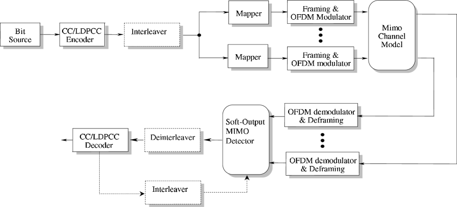
Figure 2: MIMO-OFDM BICM block diagram.

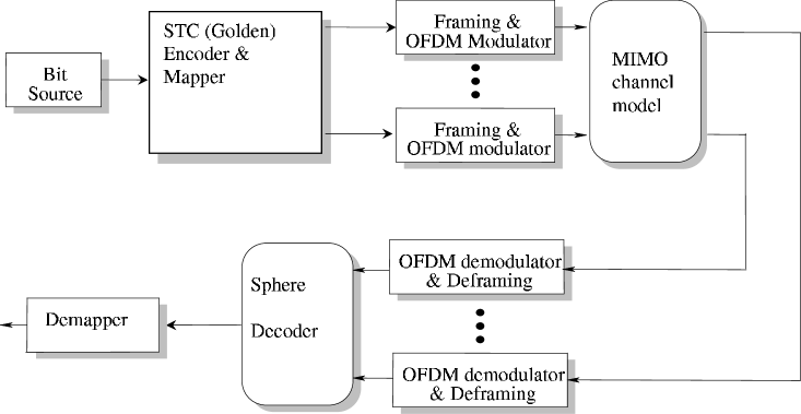
Figure 3: MIMO-OFDM STC block diagram.

In this section the performance of LORD is reported in two main MIMO-OFDM configurations of interest: BICM, which is the main scheme considered by next generation wireless standards (Fig. 2); STC mapping without concatenated ECC (Fig. 3).

Several detection algorithms have been simulated in MIMO-OFDM BICM scheme. In a subset of cases, also the performance of exhaustive-search ML detection was verified, including $L_{t}=3$ and 16QAM corresponding to 4096 operations per complex symbol. It should be noted that by ML ”exhaustive search over the constellation symbols” is meant throughout this section.

The block diagram of the system is depicted in Fig. 2. The system specifications are described in [33] and represent one of the proposals for the ongoing standardization activity of IEEE 802.11n next generation WLANs. In particular, the OFDM parameters are: 54 data tones out of a total of 64 tones; 20 MHz bandwidth; 3.2 $\mu s$ IFFT/FFT period and 0.8 $\mu s$ guard interval duration. The basic ECC scheme we considered is a convolutional code (CC) cascaded with a bit interleaver. The CC decoder is either a soft-input Viterbi algorithm (VA), or optionally a soft-in soft-out VA (SOVA, [34]) for use in turbo iterative combined decoder and detection schemes. CC performance is also compared with an advanced ECC option, i.e. a low density parity check code (LDPCC); no interleaver was used in this case. The considered LDPCC matrices are specified in [33] (1944-bit coded block size, code rates 1/2, 2/3, 3/4, 5/6); a theoretical description of their structure can be found in [35]. LDPCC simulations refer to 12 iterations of a log-domain version of the sum-product algorithm.

In order to verify the performance in different channel conditions of practical interest, two different frequency selective channel models [36] were considered: channel B, characterized by a 9-tap tapped delay line profile with 15 ns root mean square (rms) delay spread; channel D, 18-tap and 50 ns rms delay spread. Channel B is a useful benchmark for scenarios with limited frequency selectivity, like home residential environment, while Channel D has a significant frequency diversity as typical of indoor office.

The performance has been simulated in terms of packet error rate (PER) versus SNR, for a 1000-byte WLAN packet length; in the following, SNR gain will be related to $10^{-2}$ PER unless otherwise stated. The MIMO detector in Fig. 2 operates at subcarrier level, assuming known channel state information (CSI) and ideal synchronization. The following soft-output algorithms have been considered: LORD with max-log bit LLR computation; MMSE with max-log bit LLR computed taking into account the Gaussian approximation [8]; iterative MMSE and soft IC (SIC) as in [7],[8], with SOVA (optional feedback path in Fig. 2); exhaustive-search ML with optimal bit LLR computed through the Jacobian logarithm (or “$\max^{*}$” function) [30]. MMSE-SIC plots refer to four stages of MMSE processing (i.e. three iterations), as no appreciable performance improvement can be observed for more loops.

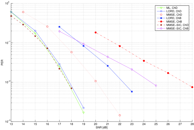
(a) 16QAM code rate 1/2

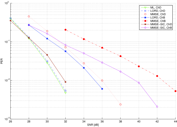
(b) 64QAM code rate 5/6

Figure 4: Performance comparison of detection algorithms. $L_{t}=2$, $L_{r}=2$ antennas, BICM MIMO-OFDM, convolutional code, channel B and D.

Fig. 4 reports the performance of LORD versus MMSE for channel models B and D, CC coded system, and $L_{t}=2$, $L_{r}=2$ (in short, 2x2) MIMO system. Fig. 4(a) and 4(b) refer to 16QAM modulation code rate (CR) 1/2 and 64QAM CR 5/6 respectively. A significant SNR gain over MMSE is visible in all cases, from a minimum of 2.2 dB for 16QAM modulation CR 1/2 and channel D, to a maximum of 7.4 dB for 64QAM CR 5/6 and channel B; also, comparisons with ML confirm the optimality of LORD with $L_{t}=2$. The small performance degradation of LORD has to be attributed to the log-MAP LLR computation used for ML as opposed to the max-log used for LORD. Interestingly, LORD and MMSE-SIC show comparable performance in case of channel D, 16QAM CR 1/2 while even a single stage of LORD gains 0.6 dB of SNR over MMSE-SIC in case of 64QAM CR 5/6. However LORD gains more than 2 dB compared to MMSE-SIC in case of channel B, 16 QAM CR 1/2 and the advantage increases to about 4.5 dB with 64QAM CR 5/6. These performance results offer several lines of interpretation. In terms of CR, the gain of LORD versus a linear suboptimal detector like MMSE increases for higher CRs. The advantage of LORD is also significantly higher when less frequency selectivity is made available by the system, as clear comparing performance obtained with channel models B and D. In particular, if limited frequency diversity exists as with channel B, MMSE-SIC does not show an appreciable BER curve slope improvement compared to a single stage of MMSE, which is the reason why LORD shows a higher gain in this condition.

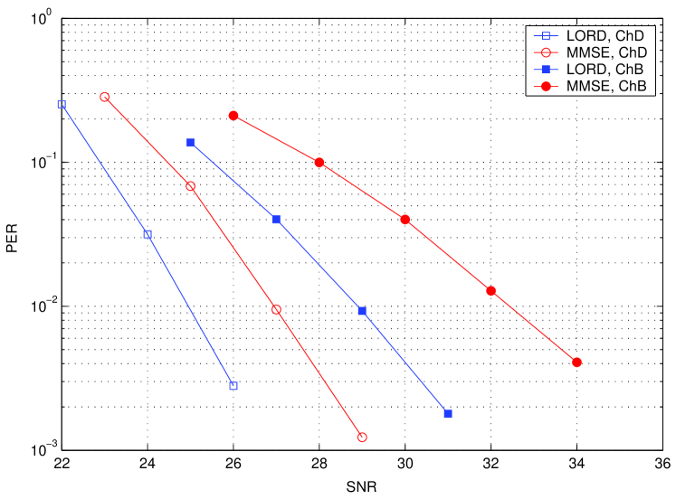
Figure 5: Performance comparison of detection algorithms. 64QAM CR 5/6, $L_{t}=2$, $L_{r}=3$, BICM MIMO-OFDM, convolutional code, channels B, D.

The performance of CC coded 64QAM, CR 5/6 is shown in Fig. 5 in case of a 2x3 MIMO system. It can be noted that the general trend visible in Fig. 4(b) still holds also if additional spatial diversity is made available by the system, even though the relative gain of LORD versus MMSE decreases; nevertheless, a SNR gain higher than 3 dB is observable for 64QAM CR 5/6 and channel model B.

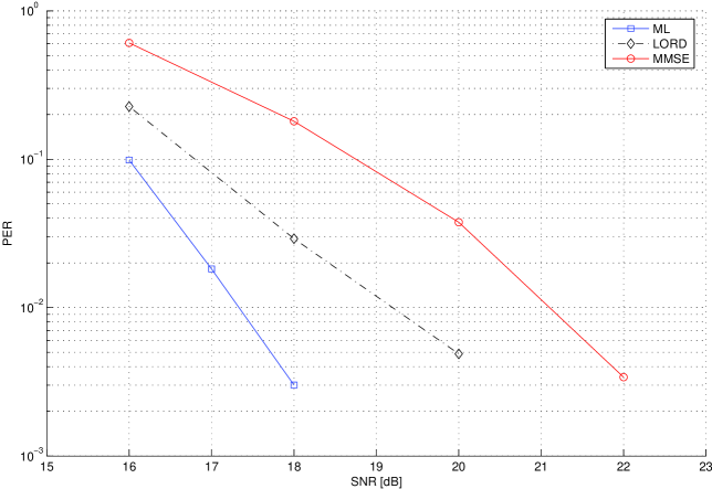
(a) 16QAM code rate 1/2

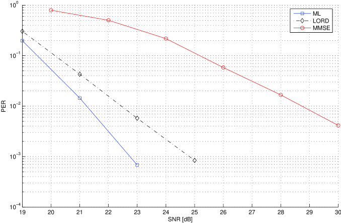
(b) 16QAM code rate 3/4

Figure 6: Performance comparison of detection algorithms. $L_{t}=3$, $L_{r}=3$, BICM MIMO-OFDM, convolutional code, channel model D.

Fig. 6-7 show that the advantage of LORD versus MMSE increases for MIMO systems with a higher number of transmit antennas (at least up to $L_{t}=4$). Fig. 6 reports the performance of 3x3 16QAM modulation, CR 1/2 and 3/4 respectively, for ML, LORD and MMSE detectors. Results confirm that LORD is suboptimal if more than two transmit antennas are used, but the gap over ML is contained within 2 dB for CR 1/2, and is only 1.2 dB for CR 3/4; in this last case the gain over MMSE is about 7.2 dB.

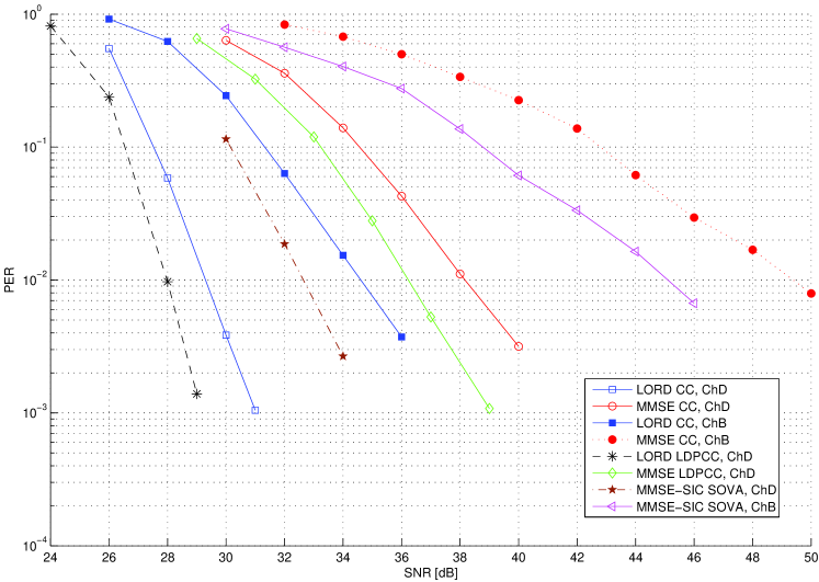
Figure 7: Performance comparison. $L_{t}=4$, $L_{r}=4$, 64QAM CR 5/6, BICM MIMO-OFDM, CC and LDPCC, channel B and D.

Fig. 7 summarizes the performance of LORD and MMSE in case of 4x4 MIMO system, 64QAM modulation, CC coded system with CR 5/6, channel models B and D; also, two plots with LDPCC and channel D are provided for comparison. The gain of LORD over MMSE is 8.9 dB and 14.8 dB with channel model D and B respectively. Also, LORD shows $>3$ dB of SNR gain over MMSE-SIC with channel D, while this gain increases to $>9$ dB if channel B is modelled. Then, LORD can avoid using iterative MMSE detectors, characterized by latency and complexity disadvantages. LORD iterative schemes are an envisioned topic for future work.

We note that even though SNR levels much higher than 30 dB are probably difficult to achieve in practical 802.11n systems, these results demonstrate the importance of a ML-approaching MIMO equalizer like LORD in order to implement the highest data rate transmission schemes currently under definition by 802.11n standardization committee (the system of Fig. 7 corresponds to a data rate of 270 Mbits/s [33]). This is particularly evident for channel model B, where MMSE has a dramatical performance degradation. It should also be observed that an advanced ECC as LDPCC is able to provide a gain over CC in the order of 2 dB if used with MMSE, and of 1.2 dB with LORD. The preliminary conclusion that can be drawn is that an advanced ECC in combination with a linear detector is not enough to recover the performance degradation of the system when limited frequency diversity is present. In this case, also iterative detection techniques do not prove to be effective if a detector unable to take advantage of receive diversity, as MMSE, is used as a first stage.

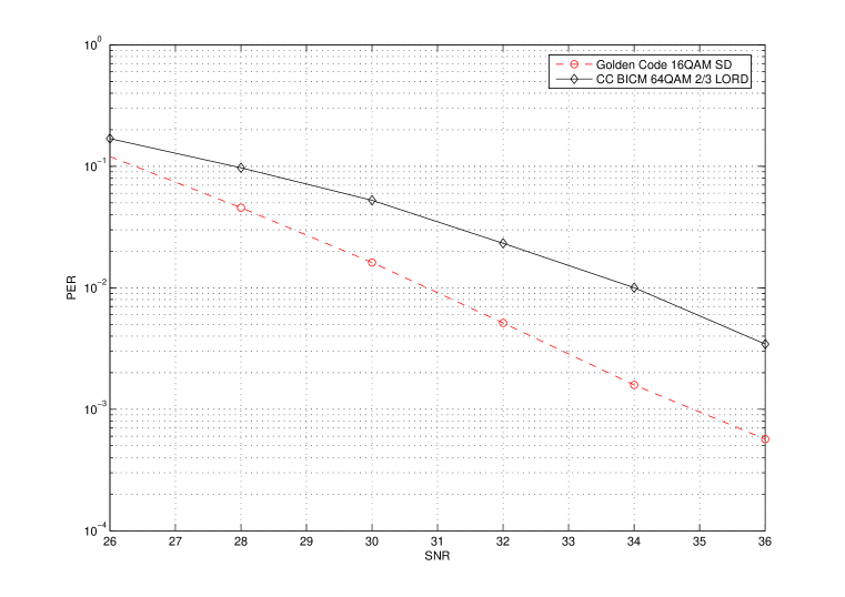
Figure 8: Performance comparison of MIMO-OFDM GC, Sphere Decoded, and CC BICM, 8 bpcu, channel model A.

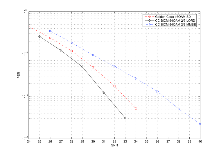
Figure 9: Performance comparison of MIMO-OFDM GC, Sphere Decoded, and CC BICM, 8 bpcu, channel model B.

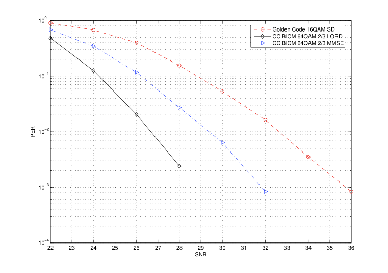
Figure 10: Performance comparison of MIMO-OFDM GC, Sphere Decoded, and CC BICM, 8 bpcu, channel model D.

Another case of interest, as previously mentioned, is represented by the algebraic STCs (ASTCs) [37],[28] in MIMO-OFDM schemes. The interest in this class of codes is motivated by their ability to yield full data rate (i.e. they transmit 2 symbols per channel use as $L_{t}=2$) and a maximal diversity order $2L_{r}$ at the same time. Particularly the Golden Codes (GCs) [28] outperform all the other classes of STCs proposed so far to the authors’ knowledge. However, ASTCs would require ML detection in order to provide full diversity order. In our simulations GCs were decoded using hard-output SD, according to the MIMO-OFDM block diagram shown in Fig. 3. The OFDM specifications were the same of the BICM system 2. MIMO-OFDM BICM LORD-detected systems outperform uncoded GCs for the same bits per channel use (bpcu), under channel conditions characterized by some degree of frequency selectivity like channel models B and D [36], as evidenced in Fig. 9 and Fig. 10 respectively for 2x2 and 8 bpcu. It should be noted that these results were obtained with 64-state CC Viterbi decoded, i.e. no powerful ECC was necessary. Only in i.i.d. flat fading channel (model A) the space-time coded system shows better performance than the BICM system (Fig. 8). Two main considerations can be drawn from these results. On one hand, they confirm the importance of a low-complexity soft-output near-ML detector like LORD in order to fully exploit the space-frequency diversity embedded in layered BICM systems as specified by practical applications like 802.11n. On the other hand, the plots also show that for short block length codes like the GCs, a hard-output ML decoder like SD is not sufficient to make them attractive for next generation wireless systems; this would still be true even if optional front-end to accelerate the decoder convergence were used, as proposed in [18]. We then infer that low-complexity soft-output near-ML detectors and a properly designed BICM scheme would be needed also for GCs in MIMO-OFDM schemes. No such detectors have been proposed so far for full diversity full data rate ASTCs; in [38] BICM TAST was decoded through a low complexity message passing iterative decoder. The adaptation of LORD to optimally decode such codes is considered a topic for future research. Advanced ECCs do not seem to be essential if enough frequency selectivity is present in the system.

VI Conclusions

In this paper a novel MIMO detection algorithm was proposed. LORD belongs to the class of lattice detector algorithms, though it uses a novel lattice formulation. A low-complexity channel preprocessing algorithm was described, alternative to the standard QR decomposition. The symbol sequence estimation is then performed through a parallelizable, reduced size and deterministic lattice search, also suitable for generation of reliable max-log bit LLRs. LORD was shown to be (max-log) optimal for two transmit antennas and near-optimal for three and four transmit sources in MIMO-OFDM BICM configuration, achieving higher SNR gain than linear and iterative nonlinear detectors, thanks to its very good exploitation of receive diversity. Also, the performance comparison with full diversity order two-transmit antenna uncoded STCs like the GCs showed that LORD detected layered BICM systems perform better even in presence of simple error correction codes like a Viterbi decoded convolutional code, provided that some degree of frequency selectivity characterizes the channel.

[Recursive formulation of the preprocessing]

The formulation for the frontend processing that was presented in Section IV-A can be given in an alternative equivalent recursive formulation. Recall the observations of interest are

$$\tilde{\textbf{y}}_{r}={\bf Q}^{T}\textbf{y}_{r}=\sqrt{\frac{E_{s}}{L_{t}}}\,{\bf\tilde{R}}\textbf{x}_{r}+{\bf Q}^{T}\textbf{n}_{r}=\sqrt{\frac{E_{s}}{L_{t}}}\,\tilde{{\bf R}}\textbf{x}_{r}+\tilde{\textbf{n}}_{r}$$ (A.78)

The orthogonal matrix can be obtained by defining the following quantities:

$$\textbf{e}_{I}(0,j)=\textbf{h}_{2j-1}\qquad\textbf{e}_{Q}(0,j)=\textbf{h}_{2j}\qquad\sigma(0,j)=\left|\textbf{h}_{2j-1}\right|^{2}\qquad 1\leq j\leq L_{t}$$ (A.79)

with the following three order recursions ($1\leq i<j\leq L_{t}$)

$$\textbf{e}_{I}(i,j) = \sigma(i-1,i)\textbf{e}_{I}(i-1,j)-r_{I}(i,j)\textbf{e}_{I}(i-1,i)-r_{Q}(i,j)\textbf{e}_{Q}(i-1,i)$$ (A.80)

$$\textbf{e}_{Q}(i,j) = \sigma(i-1,i)\textbf{e}_{Q}(i-1,j)+r_{Q}(i,j)\textbf{e}_{I}(i-1,i)-r_{I}(i,j)\textbf{e}_{Q}(i-1,i)$$ (A.81)

$$\sigma(i,j) = \sigma(i-1,i)\sigma(i-1,j)-\left(r_{I}(i,j)\right)^{2}-\left(r_{Q}(i,j)\right)^{2}$$ (A.82)

where

$$r_{I}(i,j)=\textbf{e}_{I}(i-1,i)^{T}\textbf{e}_{I}(0,j)\qquad r_{Q}(i,j)=\textbf{e}_{Q}(i-1,i)^{T}\textbf{e}_{I}(0,j).$$ (A.83)

With these definitions in place the columns of the orthogonal matrix are defined with vectors $\textbf{b}_{i}$

$$\textbf{b}_{2i-1}=\textbf{e}_{I}(i-1,i)\qquad\textbf{b}_{2i}=\textbf{e}_{Q}(i-1,i)\qquad 1\leq i\leq L_{t}.$$ (A.84)

Computing the $i^{\mbox{\scriptsize th}}$ pair of orthogonal vectors would require $i-1$ recursions of (A.80) and (A.81), each one involving $2L_{r}$ terms. However, from (A.78) and as observed in Section IV-D, the matrix ${\bf Q}$ does not actually have to be computed to accomplish detection. The vectorial recursions specified above are important in computing terms that only appear in scalar products which, in their turn, can be expressed as linear combinations of the initialization scalar vectors

$$r_{I0}(i,j)=\textbf{e}_{I}(0,i)^{T}\textbf{e}_{I}(0,j)\qquad r_{Q0}(i,j)=\textbf{e}_{Q}(0,i)^{T}\textbf{e}_{I}(0,j)\qquad 1\leq i<j\leq L_{t}.$$ (A.85)

The upper triangular matrix that results from the decomposition is also simply specified. The diagonal elements of ${\bf\tilde{R}}$ have the form:

$$\tilde{R}_{2i-1,2i-1}=\sigma(i-1,i)=\tilde{R}_{2i,2i}.$$ (A.86)

The upper triangular elements are:

$$\tilde{R}_{2i-1,2j-1}=r_{I}(i,j)\qquad\tilde{R}_{2i-1,2j}=r_{Q}(i,j)\qquad 1\leq i<j\leq L_{t}$$ (A.87)

and

$$\tilde{R}_{2i,2j-1}=-r_{Q}(i,j)\qquad\tilde{R}_{2i,2j}=r_{I}(i,j)\qquad 1\leq i<j\leq L_{t}.$$ (A.88)

The noise, $\tilde{\textbf{n}_{r}}$, remains white and has a component-wise variance given as

$$R_{\tilde{n}_{2i-1,2i-1}}=R_{\tilde{n}_{2i,2i}}=\frac{N_{0}}{2}\prod_{j=1}^{i}\sigma(j-1,j).$$ (A.89)

These recursions give the components of the upper triangular model that are needed for the detection algorithm.

The post-processed observations are also specified with a recursion. These recursions are given as

$$y_{I}(i,j) = \sigma(i-1,i)y_{I}(i-1,j)-r_{I}(i,j)y_{I}(i-1,i)-r_{Q}(i,j)y_{Q}(i-1,i)$$ (A.90)

$$y_{Q}(i,j) = \sigma(i-1,i)y_{Q}(i-1,j)+r_{Q}(i,j)y_{I}(i-1,i)-r_{I}(i,j)y_{Q}(i-1,i)$$ (A.91)

with the following initial conditions

$$y_{I}(0,j)=\textbf{e}_{I}(0,j)^{T}\textbf{Y}_{r}\qquad y_{Q}(0,j)=\textbf{e}_{Q}(0,j)^{T}\textbf{Y}_{r}.$$ (A.92)

The final outputs for the detection will be

$$\left[\textbf{y}_{r}\right]_{2i-1}=y_{I}(i-1,i)\qquad\left[\textbf{y}_{r}\right]_{2i}=y_{Q}(i-1,i)\qquad 1\leq i\leq L_{t}.$$ (A.93)

In examining the recursions needed for the upper triangular model parameters and the observations it is apparent that the orthogonal vector pairs, $\textbf{q}_{2i-1}$ and $\textbf{q}_{2i}$, only have to be computed up to the $i\leq L_{t}-1$ level.

A couple examples will help illustrate the proposed recursions. First consider again the $L_{t}=2$ case and here the preprocessing algorithm has the following pseudo code

1. Layer 1

   1. Compute $\sigma(0,1)$ – Complexity $O(2L_{r})$,

   2. Compute $y_{I}(0,1)$ – Complexity $O(2L_{r})$,

   3. Compute $y_{Q}(0,1)$ – Complexity $O(2L_{r})$,

2. Layer 2

   1. Compute $\sigma(0,2)$ – Complexity $O(2L_{r})$,

   2. Compute $y_{I}(0,2)$ – Complexity $O(2L_{r})$,

   3. Compute $y_{Q}(0,2)$ – Complexity $O(2L_{r})$,

   4. Compute $r_{I}(1,2)$ – Complexity $O(2L_{r})$,

   5. Compute $r_{Q}(1,2)$ – Complexity $O(2L_{r})$,

   6. Compute $\sigma(1,2)$ – Complexity $O(3)$,

   7. Compute $y_{I}(1,2)$ – Complexity $O(3)$,

   8. Compute $y_{Q}(1,2)$ – Complexity $O(3)$.

Again as noted above the algorithm for $L_{t}=2$ has complexity $O(16L_{r}+9)$. For the $L_{t}=4$ case the preprocessing algorithm has the following pseudo code

1. Layer 1 - Same as $L_{t}=2$ case,

2. Layer 2 - Same as $L_{t}=2$ case,

3. Layer 3

   1. Initialization $\sigma(0,3),y_{I}(0,3),y_{Q}(0,3)$ – Complexity $O(6L_{r})$,

   2. First recursion $r_{I}(1,3),r_{Q}(1,3),\sigma(1,3),y_{I}(1,3),y_{Q}(1,3)$ – Complexity $O(4L_{r}+9)$,

   3. Second recursion $r_{I}(2,3),r_{Q}(2,3),\sigma(2,3),y_{I}(2,3),y_{Q}(2,3)$ – Complexity $O(4L_{r}+15)$,

4. Layer 4

   1. Initialization $\sigma(0,4),y_{I}(0,4),y_{Q}(0,4)$ – Complexity $O(6L_{r})$,

   2. First recursion $r_{I}(1,4),r_{Q}(1,4),\sigma(1,4),y_{I}(1,4),y_{Q}(1,4)$ – Complexity $O(4L_{r}+9)$,

   3. Second recursion $r_{I}(2,4),r_{Q}(2,4),\sigma(2,4),y_{I}(2,4),y_{Q}(2,4)$ – Complexity $O(4L_{r}+15)$,

   4. Third recursion $r_{I}(3,4),r_{Q}(3,4),\sigma(3,4),y_{I}(3,4),y_{Q}(3,4)$ – Complexity $O(4L_{r}+15)$,

The overall complexity for $L_{t}=4$ case is $O\left(48L_{r}+72\right)$. In general the complexity of the preprocessing algorithm is $O\left(2L_{r}L_{t}^{2}+4L_{t}L_{r}\right)$, the same order of magnitude reported in Section IV-D.

References

- [1] W. van Etten, “Maximum likelihood receiver for multiple channel transmission systems,” IEEE Trans. Commun., vol. 24, no. 2, pp. 276–283, Feb. 1976.
- [2] S. Verdú, Multiuser Detection. Cambridge University Press, 1998.
- [3] R. van Nee, A. van Zelst, and G. Awater, “Maximum likelihood decoding in a space division multiplexing system,” in Proc. IEEE Vehicular Tech. Conf., vol. 1, May 2000, pp. 6–10.
- [4] P. W. Wolniansky, G. J. Foschini, G. D. Golden, and R. A. Valenzuela, “V-BLAST: An architecture for realizing very high data rates over the rich-scattering wireless channel,” in Proc. URSI International Symposium on Signals, Systems, and Electronics, Sep. 1998, pp. 295–300.
- [5] G. J. Foschini, G. D. Golden, R. A. Valenzuela, and P. W. Wolniansky, “Simplified processing for high spectral efficiency wireless communications employing multi-element arrays,” IEEE J. Select. Areas Commun., vol. 17, no. 11, pp. 1841–1852, Nov. 1999.
- [6] K.-B. Song and S. A. Mujtaba, “A low complexity space-frequency BICM MIMO-OFDM system for next-generation WLANs,” in Proc. IEEE Global Telecommunications Conf., 2003, pp. 1059–1063.
- [7] M. Sellathurai and S. Haykin, “Turbo-BLAST for wireless communications: Theory and experiments,” IEEE Trans. Signal Processing, vol. 50, pp. 2538–2546, Oct. 2002.
- [8] D. Zuyderhoff, X. Wautelet, A. Dejonghe, and L. Vandendorpe, “MMSE turbo receiver for space-frequency bit-interleaved coded OFDM,” in Proc. IEEE Vehicular Tech. Conf., vol. 1, Oct. 2003, pp. 567–571.
- [9] W.-J. Choi, R. Negri, and J. M. Cioffi, “Combined ML and DFE decoding for the V-BLAST system,” in Proc. IEEE Int. Conf. Communications, vol. 3, June 2000, pp. 1243–1248.
- [10] Y. Li and Z.-Q. Luo, “Parallel detection for V-BLAST system,” in Proc. IEEE Global Telecommunications Conf., vol. 1, May 2002, pp. 340–344.
- [11] D. W. Waters and J. R. Barry, “The Chase family of detection algorithms for multiple-input multiple-ouput channels,” in Proc. IEEE Global Telecommunications Conf., vol. 4, Nov. 2004, pp. 2635–2639.
- [12] ——, “The Chase family of detection algorithms for multiple-input multiple-ouput channels,” Submitted to IEEE Trans. Info. Theory, Sep. 2005.
- [13] H. Sung, K. B. E. Lee, and J. W. Kang, “A simplified maximum likelihood detection scheme for MIMO systems,” in Proc. IEEE Vehicular Tech. Conf., vol. 1, Oct. 2003, pp. 419–423.
- [14] E. Viterbo and J. Boutros, “A universal lattice code decoder for fading channels,” IEEE Trans. Info. Theory, vol. 1, no. 5, pp. 1639–1642, July 1999.
- [15] E. Agrell, T. Eriksson, A. Vardy, and K. Zeger, “Closest point search in lattices,” IEEE Trans. Info. Theory, vol. 48, no. 8, pp. 2201–2214, Aug. 2002.
- [16] M. O. Damen, A. Chkeif, and J.-C. Belfiore, “Lattice codes decoder for space-time codes,” IEEE Commun. Letters, vol. 4, no. 5, pp. 161–163, May 2000.
- [17] M. O. Damen, E. Gamal, and G. Caire, “On maximum-likelihood detection and the search for the closest lattice point,” IEEE Trans. Info. Theory, vol. 49, no. 10, pp. 2389–2402, Oct. 2003.
- [18] A. D. Murugan, E. Gamal, M. O. Damen, and G. Caire, “A unified framework for tree search decoding: Rediscovering the sequential decoder,” To appear in IEEE Trans. Info. Theory, May 2005.
- [19] J. Jalden and B. Ottersten, “On the complexity of sphere decoding in digital communications,” IEEE Trans. Signal Processing, vol. 53, no. 4, pp. 1474–1484, Apr. 2005.
- [20] A. K. Lenstra, A. W. L. Jr., and L. Lovász, “On factoring polynomials with rational coefficients,” Math. Annalen., vol. 261, pp. 515–534, 1982.
- [21] C. P. Schnorr and M. Euchner, “Lattice basis reduction: improved practical algorithms and solving subset sum problems,” Math. Programming, vol. 66, pp. 181–191, 1994.
- [22] B. Hochwald and S. ten Brink, “Achieving near-capacity on a multiple-antenna channel,” IEEE Trans. Commun., vol. 51, no. 3, pp. 389–399, Mar. 2003.
- [23] J. Boutros, N. Gresset, L. Brunel, and M. Fossorier, “Soft-input soft-output lattice sphere decoder for linear channels,” in Proc. IEEE Global Telecommunications Conf., vol. 3, Dec. 2003, pp. 1583–1587.
- [24] E. Zimmermann, W. Rave, and G. Fettweis, “On the complexity of sphere decoding,” in Proc. International Symp. on Wireless Pers. Multimedia Commun., Abano Terme, Italy, Sep. 2004.
- [25] D. Shiu and J. M. Kahn, “Layered space-time codes for wireless communications using multiple transmit antennas,” in Proc. IEEE Int. Conf. Communications, Vancouver, Canada, June 1999.
- [26] M. Siti and M. P. Fitz, “Layered orthogonal lattice detector for two transmit antenna communications,” in Proc. Allerton Conference On Communication, Control, And Computing, Sep. 2005.
- [27] ——, “A novel soft-ouput layered orthogonal lattice detector for multiple antenna communications,” in To appear in Proc. IEEE Int. Conf. On Commun., 2006.
- [28] J. C. Belfiore, G. Rekaya, and E. Viterbo, “The golden code: a 2x2 full-rate space-time code with non-vanishing determinants,” IEEE Trans. Info. Theory, vol. 51, no. 4, pp. 1432–1436, Apr. 2005.
- [29] IEEE P802.11n/D0.02, “Draft Amendment to Standard for Information Technology-Telecommunications-and information exchange between systems-Local and Metropolitan Networks-Specific requirements-Part 11: Wireless LAN Medium Access Control (MAC) and Physical Layer (PHY) specification: Enhancements for Higher Throughput,” IEEE Standards Activities Department, Tech. Rep., February 2006.
- [30] P. Robertson, E. Villebrun, , and P. Hoeher, “A comparison of optimal and sub-optimal MAP decoding algorithms operating in the log domain communications,” in Proc. IEEE Int. Conf. Communications, vol. 2, June 1995, pp. 1009–1013.
- [31] G. H. Golub and C. F. Van Loan, Matrix Computations, 3rd ed. Baltimore, MD: Johns Hopkins University Press, 1996.
- [32] A. Burg, M. Borgmann, M. Wenk, M. Zellweger, W. Fichtner, and H. Bolcskei, “VLSI implementation of MIMO detection using the sphere decoding algorithm,” IEEE Journ. Solid-State Circuits, vol. 40, no. 7, pp. 1566–1577, July 2005.
- [33] IEEE 802.11-04/0886r6, “WWiSE Proposal: High throughput extension to the 802.11 Standard,” Tech. Rep., January 2005.
- [34] J. Hagenauer and P. Hoeher, “A Viterbi algorithm with soft-decision outputs and its applications,” in Proc. IEEE Global Telecommunications Conf., vol. 3, Dallas, TX, Nov. 1989, pp. 1680–1686.
- [35] A. I. Vila Casado, W.-Y. Weng, and R. Wesel, “Multiple rate low-density parity-check codes with constant blocklength,” in Proc. Asilomar Conf. Signals, Systems, and Computers, 2004.
- [36] V. Erceg et al., “IEEE 802.11 TGn channel models, Tech. Rep. IEEE 802.11-03/940r1, January 2004.
- [37] O. Damen, A. Tewfik, and J. C. Belfiore, “A construction of a space-time code based on algebraic number theory,” IEEE Trans. Info. Theory, vol. 48, no. 3, pp. 753–760, Mar. 2002.
- [38] A. G. i Fabregas and G. Caire, “Impact of signal constellation expansion on the achievable diversity of pragmatic bit-interleaved space-time codes,” To appear in IEEE Trans. Wireless Commun., Oct. 2004.