Solving Sparse Integer Linear Systems

Abstract

We propose a new algorithm to solve sparse linear systems of equations over the integers. This algorithm is based on a $p$-adic lifting technique combined with the use of block matrices with structured blocks. It achieves a sub-cubic complexity in terms of machine operations subject to a conjecture on the effectiveness of certain sparse projections. A LinBox -based implementation of this algorithm is demonstrated, and emphasizes the practical benefits of this new method over the previous state of the art.

1 Introduction

A fundamental problem of linear algebra is to compute the unique solution of a non-singular system of linear equations. Aside from its importance in and of itself, it is key component in many recent proposed algorithms for other problems involving exact linear systems. Among those algorithms are Diophantine system solving [10, 19, 20], Smith form computation [8, 21], and null-space and kernel computation [3]. In its basic form, the problem we consider is then to compute the unique rational vector $A^{-1}b\in{\mathbb{Q}}^{n\times 1}$ for a given non-singular matrix $A\in{\mathbb{Z}}^{n\times n}$ and right hand side $b\in{\mathbb{Z}}^{n\times 1}$. In this paper we give new and effective techniques for when $A$ is a sparse integer matrix, which have sub-cubic complexity on sparse matrices.

A classical and successful approach to solving this problem for dense integer matrices $A$ was introduced by Dixon in 1982 [5], following polynomial case studies from [18]. His proposed technique is to compute, iteratively, a sufficiently accurate $p$-adic approximation $A^{-1}b\bmod p^{k}$ of the solution. The prime $p$ is chosen such that $\det(A)\mskip 4.0mu\not\equiv\mskip 4.0mu0\bmod p$ (see, e.g., [22] for details on the choice of $p$). Then, using radix conversion (see e.g. [9, §12]) combined with continued fraction theory [13, §10], one can easily reconstruct the rational solution $A^{-1}b$ from $A^{-1}b\bmod p^{k}$ (see [25] for details).

The principal feature of Dixon’s technique is the pre-computation of the matrix $A^{-1}\bmod p$ which leads to a decreased cost of each lifting step. This leads to an algorithm with a complexity of ${O{\;\!\tilde{}}\,}(n^{3}\log(\|A\|+\|b\|))$ bit operations [5]. Here and in the rest of this paper $\|\ldots\|$ denotes the maximum entry in absolute value and the ${O{\;\!\tilde{}}\,}$ notation indicates some possibly omitting logarithmic factor in the variables.

For a given non-singular matrix $A\in{\mathbb{Z}}^{n\times n}$, a right hand side $b\in{\mathbb{Z}}^{n\times 1}$, and a suitable integer $p$, Dixon’s scheme is the following:

• compute $B=A^{-1}\bmod p$;

• compute $\ell$ $p$-adic digits of the approximation iteratively by multiplying $B$ times the right hand side, which is updated according to each new digit;

• use radix conversion and rational number reconstruction to recover the solution.

The number $\ell$ of lifting steps required to find the exact rational solution to the system is ${O{\;\!\tilde{}}\,}(n\log(\|A\|+\|b\|))$, and one can easily obtain the announced complexity (each lifting steps requires a quadratic number of bit operations in the dimension of $A$; see [5] for more details).

In this paper we study the case when $A$ is a sparse integer matrix, for example, when only ${O{\;\!\tilde{}}\,}(n)$ entries are non-zero. The salient feature of such a matrix $A$ is that applying $A$, or its transpose, to a dense vector $c\in{\mathbb{Z}}^{n\times 1}$ requires only ${O{\;\!\tilde{}}\,}(n\log(\|A\|+\|c\|))$ bit operations.

Following techniques proposed by Wiedemann in [26], one can compute a solution of a sparse linear system over a finite field in ${O{\;\!\tilde{}}\,}(n^{2})$ field operations, with only ${O{\;\!\tilde{}}\,}(n)$ memory. Kaltofen & Saunders [16] studied the use of Wiedemann’s approach, combined with $p$-adic approximation, for sparse integer linear system. Nevertheless, this combination doesn’t help to improve the bit complexity compared to Dixon’s algorithm: it still requires ${O{\;\!\tilde{}}\,}(n^{3})$ operations in the worst case. One of the main reasons is that Wiedemann’s technique requires the computation, for each right hand side, of a new Krylov subspace, which requires $O(n)$ matrix-vector products by $A\bmod p$. This implies the requirement of $\Theta(n^{2})$ operations modulo $p$ for each lifting step, even for a sparse matrix (and $\Theta(n(\log\|A\|+\|b\|))$ such lifting steps are necessary in general). The only advantage then of using Wiedemann’s technique is memory management: only $O(n)$ additional memory is necessary, as compared to the $O(n^{2})$ space needed to store matrix inverse modulo $p$ explicitly, which may well be dense even for sparse $A$.

The main contribution of this current paper is to provide a new Krylov-like pre-computation for the $p$-adic algorithm with a sparse matrix which allows us to improve the bit complexity of linear system solving. The main idea is to use block-Krylov method combined with special block projections to minimize the cost of each lifting step. The Block Wiedemann algorithm [4, 24, 14] would be a natural candidate to achieve this. However, the Block Wiedemann method is not obviously suited to being incorporated into a $p$-adic scheme. Unlike the scalar Wiedemann algorithm, wherein the minimal polynomial can be used for every right-hand side, the Block Wiedemann algorithm needs to use different linear combinations for each right-hand side. In particular, this is due to the special structure of linear combinations coming from a column of a minimal matrix generating polynomial (see [24, 23]) and then be totally dependent on the right hand side.

Our new scheme reduces the cost of each lifting step, on a sparse matrix as above, to ${O{\;\!\tilde{}}\,}(n^{1.5})$ bit operations. This means the cost of the entire solver is ${O{\;\!\tilde{}}\,}(n^{2.5}(\log(\|A\|+\|b\|))$ bit operations. The algorithm makes use of the notion of an efficient sparse projection, for which we currently only offer a construction which is conjectured to work in all cases. However, we do provide some theoretical evidence to support its applicability, and note its effectiveness in practice.

Most importantly, the new algorithm is shown to offer significant practical improvement on sparse integer matrices. The algorithm is implemented in the LinBox library [6], a generic C++ library for exact linear algebra. We compare it against the best known solvers for integer linear equations, in particular against the Dixon lifting scheme and Chinese remaindering. We show that in practice it runs many times faster than previous schemes on matrices of size greater than $2500\times 2500$ with suffiently high sparsity. This also demonstrates the effectiveness in practice of so-called “asymptotically fast” matrix-polynomial techniques, which employ fast matrix/polynomial arithmetic. We provide a detailed discussion of the implementation, and isolate the performance benefits and bottlenecks. A comparison with Maple dense solver emphasizes the high efficiency of the LinBox library and the needs of well-designed sparse solvers as well.

2 Block projections

The basis for Krylov-type linear algebra algorithms is the notion of a projection. In Wiedemann’s algorithm, for example, we solve the ancillary problem of finding the minimal polynomial of a matrix $A\in{\sf F}^{n\times n}$ over a field ${\sf F}$ by choosing random $u\in{\sf F}^{1\times n}$ and $v\in{\sf F}^{n\times 1}$ and computing the minimal polynomial of the sequence $uA^{i}v$ for $i=0..2n-1$ (which is both easy to compute and with high probability equals the minimal polynomial of $A$). As noted in the introduction, our scheme will ultimately be different, a hybrid Krylov and lifting scheme, but will still rely on the notion of a structured block projection.

For the remainder of the paper, we adopt the following notation:

• $A\in{\sf F}^{n\times n}$ be a non-singular matrix,

• $s$ be a divisor of $n$, the blocking factor, and

• $m:=n/s$.

Ultimately ${\sf F}$ will be ${\mathbb{Q}}$ and we will have $A\in{\mathbb{Z}}^{n\times n}$, but for now we work in the context of a more general field ${\sf F}$.

For a block $v\in{\sf F}^{n\times s}$ and $0\leq t\leq m$, define

$${\mathcal{K}}(A,v):=\left[\begin{array}[]{c|c|c|c}v&Av&\cdots&A^{m-1}v\end{array}\right]\in{\sf F}^{n\times n}.$$

We call a triple $(R,u,v)\in{\sf F}^{n\times n}\times{\sf F}^{s\times n}\times{\sf F}^{n\times s}$ an efficient block projection if and only if

1. ${\mathcal{K}}(AR,v)$ and ${\mathcal{K}}((AR)^{T},u^{T})$ are non-singular;

2. $R$ can be applied to a vector with ${O{\;\!\tilde{}}\,}(n)$ operations in ${\sf F}$;

3. we can compute $vx$, $u^{T}x$, $yv$ and $yu^{T}$ for any $x\in{\sf F}^{s\times 1}$ and $y\in{\sf F}^{1\times n}$, with ${O{\;\!\tilde{}}\,}(n)$ operations in ${\sf F}$.

In practice we might hope that $R$, $u$ and $v$ in an efficient block projection are extremely simple, for example $R$ is a diagonal matrix and $u$ and $v$ have only $n$ non-zero elements.

Conjecture 2.1.

For any non-singular $A\in{\sf F}^{n\times n}$ and $s{\mskip 3.0mu|\mskip 3.0mu}n$, there exists an efficient block projection $(R,u,v)\in{\sf F}^{n\times n}\times{\sf F}^{s\times n}\times{\sf F}^{n\times s}$, and it can be constructed quickly.

2.1 Constructing efficient block projections

In what follows we present an efficient sparse projection which we conjecture to be effective for all matrices. We also present some supporting evidence (if not proof) for its theoretical effectiveness. As we shall see in Section 4, the projection performs extremely well in practice.

We focus only on $R$ and $v$, since its existence should imply the existence of a $u$ of similar structure.

For convenience, assume for now that all elements in $v$ and $R$ are algebraically independent indeterminates, modulo some imposed structure. This is sufficient, since the existence of an efficient sparse projection with indeterminate entries would imply that a specialization to an effective sparse projection over ${\mathbb{Z}}_{p}$ is guaranteed to work with high probability, for sufficiently large $p$. We also consider some different possibilities for choosing $R$ and $v$.

2.1.1 Dense Projections

The “usual” scheme for block matrix algorithms is to choose $R$ diagonal, and $v$ dense. The argument to show this works has several steps. First, $AR$ will have distinct eigenvalues and thus will be non-derogatory (i.e., its minimal polynomial equals its characteristic polynomial). See [2], Lemma 4.1. Second, for any non-derogatory matrix $B$ and dense $v$ we have ${\mathcal{K}}(B,v)$ non-singular (see [15]). However, a dense $v$ is not an efficient block projection since condition (2) is not satisfied.

2.1.2 Structured Projections

The following projection scheme is the one we use in practice. Its effectiveness in implementation is demonstrated in Section 4.

Choose $R$ diagonal as before. Choose

$$v=\left[\begin{array}[]{c|c|c|c}\ast&&&\\ \hline\cr&\ast&&\\ \hline\cr&&\ddots&\\ \hline\cr&&&\ast\end{array}\right]\in k^{n\times s}$$ (1)

with each $\ast$ of dimension $m\times 1$. The intuition behind the structure of $v$ is twofold. First, if $s=1$ then $v$ is a dense column vector, and we know ${\mathcal{K}}(AR,v)$ is non-singular in this case. Second, since the case $s=1$ requires only $n$ nonzero elements in the “block”, it seems that $n$ nonzero elements should suffice in the case $s>1$ also. Third, if $E$ is a diagonal matrix with distinct eigenvalues then, up to a permutation of the columns, ${\mathcal{K}}(E,v)$ is a block Vandermonde matrix, each $m\times m$ block defined via $m$ distinct roots, thus non-singular. In the general case with $s>1$ we ask:

Question 2.2.

For $R$ diagonal and $v$ as in (1), is ${\mathcal{K}}(AR,v)$ necessarily nonsingular?

Our work thus far has not led to a resolution of the question. However, by focusing on the case $s=2$ we have answered the following similar question negatively: If $A$ is nonsingular with distinct eigenvalues and $v$ is as in (1), is ${\mathcal{K}}(A,v)$ necessarily nonsingular?

Lemma 2.3.

If $m=2$ there exists a nonsingular $A$ with distinct eigenvalues such that for $v$ as in (1) the matrix ${\mathcal{K}}(A,v)$ is singular.

Proof.

We give a counterexample with $n=4$. Let

$$E=\left[\begin{array}[]{cccc}1&0&0&0\\ \vskip 6.0pt plus 2.0pt minus 2.0pt\cr 0&2&0&0\\ \vskip 6.0pt plus 2.0pt minus 2.0pt\cr 0&0&3&0\\ \vskip 6.0pt plus 2.0pt minus 2.0pt\cr 0&0&0&4\end{array}\right]\hbox{~{}~{}and~{}~{}}P=\left[\begin{array}[]{cccc}1&0&0&0\\ \vskip 6.0pt plus 2.0pt minus 2.0pt\cr 0&1&1/4&0\\ \vskip 6.0pt plus 2.0pt minus 2.0pt\cr 0&1&1&0\\ \vskip 6.0pt plus 2.0pt minus 2.0pt\cr 0&0&0&1\end{array}\right].$$

Define

$$A=3P^{-1}EP=\left[\begin{array}[]{cccc}3&0&0&0\\ \vskip 6.0pt plus 2.0pt minus 2.0pt\cr 0&5&-1&0\\ \vskip 6.0pt plus 2.0pt minus 2.0pt\cr 0&4&10&0\\ \vskip 6.0pt plus 2.0pt minus 2.0pt\cr 0&0&0&12\end{array}\right].$$

For the generic block

$$v=\left[\begin{array}[]{cc}a_{1}&\\ a_{2}\\ &b_{1}\\ &b_{2}\end{array}\right]$$

the matrix ${\mathcal{K}}(A,v)$ is singular. By embedding $A$ into a larger block diagonal matrix we can construct a similar counterexample for any $n$ and $m=2$. ∎

Thus, if Question 2.2 has an affirmative answer, then proving it will necessitate considering the effect of the diagonal preconditioner $R$ above and beyond the fact that “$AR$ has distinct eigenvalues”. For example, are the eigenvalues of $AR$ algebraically independent, using the fact that entries in $R$ are? This may already be sufficient.

2.1.3 A Positive Result for the Case $s=2$

For $s=2$ we can prove the effectiveness of our efficient sparse projection scheme.

Suppose that $A\in{\sf F}^{n\times n}$ where $n$ is even and $A$ is diagonalizable with distinct eigenvalues in an extension of ${\sf F}$. Then $A=X^{-1}DX\in{\sf F}^{n\times n}$ for some diagonal matrix $D$ with distinct diagonal entries (in this extension). Note that the rows of $X$ can be permuted (replacing $X$ with $PX$ for some permutation $P$),

$$A=((PX)^{-1}(P^{-1}DP)(PX)),$$

and $P^{-1}DP$ is also a diagonal matrix with distinct diagonal entries. Consequently we may assume without loss of generality that the top left $(n/2)\times(n/2)$ submatrix $X_{1,1}$ of $X$ is nonsingular. Suppose that

$$X=\left[\begin{array}[]{cc}X_{1,1}&X_{1,2}\\ X_{2,1}&X_{2,2}\end{array}\right]$$

and consider the decomposition

$$A=Z^{-1}\widehat{A}Z,$$ (2)

where

$$Z=\left[\begin{array}[]{cc}X_{1,1}^{-1}&0\\ 0&X_{1,1}^{-1}\end{array}\right]\quad X=\left[\begin{array}[]{cc}I&Z_{1,2}\\ Z_{2,1}&Z_{2,2}\end{array}\right]$$

for $n/2\times n/2$ matrices $Z_{1,2}$, $Z_{2,1}$, and $Z_{2,2}$, and where

$$\widehat{A}=\left[\begin{array}[]{cc}X_{1,1}^{-1}&0\\ 0&X_{1,1}^{-1}\end{array}\right]D\left[\begin{array}[]{cc}X_{1,1}&0\\ 0&X_{1,1}\end{array}\right],$$

so that

$$\widehat{A}=\left[\begin{array}[]{cc}A_{1}&0\\ 0&A_{2}\end{array}\right],$$

for matrices $A_{1}$ and $A_{2}$. The matrices $A_{1}$ and $A_{2}$ are each diagonalizable over an extension of ${\sf F}$, since $A$ is, and the eigenvalues of these matrices are also distinct.

Notice that, for vectors $a,b$ with dimension $n/2$, and for any nonnegative integer $i$,

$$A^{i}\left[\begin{array}[]{c}a\\ 0\end{array}\right]=Z^{-1}\widehat{A}^{i}\left[\begin{array}[]{c}a\\ Z_{2,1}a\end{array}\right]\quad\mbox{and}\quad A^{i}\left[\begin{array}[]{c}0\\ b\end{array}\right]=Z^{-1}\widehat{A}^{i}\left[\begin{array}[]{c}Z_{1,2}b\\ Z_{2,2}b\end{array}\right].$$

Thus, if

$$x=\left[\begin{array}[]{cc}a\\ Z_{2,1}a\end{array}\right]\quad\mbox{and}\quad y=\left[\begin{array}[]{cc}Z_{1,2}b\\ Z_{2,2}b\end{array}\right]$$

then the matrix with columns

$$a,Aa,A^{2}a,\ldots,A^{n/2-1}a,b,Ab,A^{2}b,\ldots,A^{n-2-1}b$$

is nonsingular if and only if the matrix with columns

$$x,\widehat{A}x,\widehat{A}^{2}x,\ldots,\widehat{A}^{n/2-1}x,y,\widehat{A}y,\widehat{A}^{2}y,\ldots,\widehat{A}^{n/2-1}y$$

is nonsingular. The latter condition fails if and only if there exist polynomials $f$ and $g$, each with degree less than $n/2$, such that at least one of these polynomials is nonzero and

$$f(\widehat{A})x+g(\widehat{A})y=0.$$ (3)

To proceed, we should therefore determine a condition on $A$ ensuring that no such polynomials $f$ and $g$ exist for some choice of $x$ and $y$ (that is, for some choice of $a$ and $b$).

A suitable condition on $A$ is easily described: We will require that the top right submatrix $Z_{1,2}$ of $Z$ is nonsingular.

Now suppose that the entries of the vector $b$ are uniformly and randomly chosen from some (sufficiently large) subset of ${\sf F}$, and suppose that $a=-Z_{1,2}b$. Notice that at least one of $f$ and $g$ is nonzero if and only if at least one of $f$ and $g-f$ is nonzero. Furthermore,

$$f(\widehat{A})(x)+g(\widehat{A})(y)=f(\widehat{A})(x+y)+(g-f)(\widehat{A})(y).$$

It follows by the choice of $a$ that

$$x+y=\left[\begin{array}[]{cc}0\\ (Z_{2,2}-Z_{2,1}Z_{1,2})b\end{array}\right].$$

Since $\widehat{A}$ is block diagonal, the top $n/2$ entries of $f(\widehat{A})(x+y)$ are nonzero as well for every polynomial $f$. Consequently, failure condition (3) can only be satisfied if the top $n/2$ entries of the vector $(g-f)(\widehat{A})(y)$ are also all zero.

Recall that $g-f$ has degree less than $n/2$ and that the top left submatrix of the block diagonal matrix $\widehat{A}$ is diagonalizable with $n/2$ distinct eigenvalues. Assuming, as noted above, that $Z_{1,2}$ is nonsingular (and recalling that the top half of the vector $y$ is $Z_{1,2}b$), the Schwartz-Zippel lemma is easily used to show that if $b$ is randomly chosen as described then, with high probability, the failure condition can only be satisfied if $g-f=0$. That is, it can only be satisfied if $f=g$.

Observe next that, in this case,

$$f(\widehat{A})(x)+g(\widehat{A})(y)=f(\widehat{A})(x+y),$$

and recall that the bottom half of the vector $x+y$ is the vector $(Z_{2,2}-Z_{2,1}Z_{1,2})b$. The matrix $Z_{2,2}-Z_{2,1}Z_{1,2}$ is clearly nonsingular (it is a Schur complement formed from $Z$) so, once again, the Schwartz-Zippel lemma can be used to show that if $b$ is randomly chosen as described above then $f(\widehat{A})(x+y)=0$ if and only if $f=0$ as well.

Thus if $Z_{1,2}$ is nonsingular and $a$ and $b$ are chosen as described above then, with high probability, equation (3) is satisfied only if $f=g=0$. There must therefore exist a choice of $a$ and $b$ providing an efficient block projection — once again, supposing that $Z_{1,2}$ is nonsingular.

It remains only to describe a simple and efficient randomization of $A$ that achieves this condition with high probability: Let us replace $A$ with the matrix

$$\widetilde{A}=\left[\begin{array}[]{cc}I&tI\\ 0&I\end{array}\right]^{-1}A\left[\begin{array}[]{cc}I&tI\\ 0&I\end{array}\right]=\left[\begin{array}[]{cc}I&-tI\\ 0&I\end{array}\right]A\left[\begin{array}[]{cc}I&tI\\ 0&I\end{array}\right],$$

where $t$ is chosen uniformly from a sufficiently large subset of ${\sf F}$. This has the effect of replacing $Z$ with the matrix

$$Z\left[\begin{array}[]{cc}I&tI\\ 0&I\end{array}\right]=\left[\begin{array}[]{cc}I&Z_{1,2}+tI\\ Z_{2,1}&Z_{2,2}+tZ_{2,1}\end{array}\right]$$

(see, again, (2)), effectively replacing $Z_{1,2}$ with $Z_{1,2}+tI$. There are clearly at most $n/2$ choices of $t$ for which the latter matrix is singular.

Finally, note that if $v$ is a vector and $i\geq 0$ then

$$\widetilde{A}^{i}v=\left[\begin{array}[]{cc}I&-tI\\ 0&I\end{array}\right]A^{i}\left[\begin{array}[]{cc}I&tI\\ 0&I\end{array}\right]v.$$

It follows by this and similar observations that this randomization can be applied without increasing the asymptotic cost of the algorithm described in this paper.

Question: Can the above randomization and proof be generalized to a similar result for larger $s$?

Other sparse block projections

Other possible projections are summarized as follows.

• Iterative Choice Projection. Instead of choosing $v$ all at once, choose the columns of $v=[v_{1}|v_{2}|\cdots|v_{s}]$ in succession. For example, suppose up to preconditioning we can assume we are working with a $B\in{\sf F}^{n\times n}$ that is simple as well as has the property that the characteristic polynomial is irreducible. Then we can choose $v_{1}$ to be the first column of $I_{n}$ to achieve ${\mathcal{K}}(B,v_{1})\in{\sf F}^{n\times m}$ of rank $m$. Next choose $v_{2}$ to have two nonzero entries, locations chosen randomly until $[{\mathcal{K}}(B,v_{1})|{\mathcal{K}}(B,v_{2})]\in{\sf F}^{n\times 2m}$ has rank $2m$, etc. This gives a $v$ with $m(m+2)/2$ nonzero entries.

  The point of choosing $v$ column by column is that, while choosing all of $v$ sparse may have a very small probability of success, the success rate for choosing $v_{i}$ when $v_{1},v_{2},\ldots,v_{i-1}$ are already chosen may be high enought (e.g., maybe only expected $O(\log n))$ choices for $v_{i}$ before success).

• Toeplitz projections. Choose $R$ and/or $v$ to have a Toeplitz structure.

• Vandermonde projections. Choose $v$ to have a Vandermonde or a Vandermonde-like structure.

3 Non-singular sparse solver

In this section we show how to employ a block-Krylov type method combined with the (conjectured) efficient block projections of Section 2 to improve the complexity of evaluating the inverse modulo $p$ of a sparse matrix. Applying Dixon’s $p$-adic scheme with such an inverse yields an algorithm with better complexity than previous methods for sparse matrices, i.e., those with a fast matrix-vector product. In particular, we express the cost of our algorithm in terms of the number of applications of the input matrix to a vector, plus the number of auxiliary operations.

More precisely, given $A\in{\mathbb{Z}}^{n\times n}$ and $v\in{\mathbb{Z}}^{n\times 1}$, let $\mu(n)$ be the number of operations in ${\mathbb{Z}}$ to compute $Av$ or $v^{T}A$. Then, assuming Conjecture 2.1, our algorithm requires ${O{\;\!\tilde{}}\,}(n^{1.5}(\log(\|A\|+\|b\|))$ matrix-vector products $w\mapsto Aw$ on vectors $w\in{\mathbb{Z}}^{n\times 1}$ with $\|w\|=O(1)$, plus ${O{\;\!\tilde{}}\,}(n^{2.5}(\log(\|A\|+\|b\|))$ additional bit operations.

Summarizing this for practical purposes, in the common case of a matrix $A\in{\mathbb{Z}}^{n\times n}$ with ${O{\;\!\tilde{}}\,}(n)$ constant-sized non-zero entries, and $b\in{\mathbb{Z}}^{n\times 1}$ with constant-sized entries, we can compute $A^{-1}b$ with ${O{\;\!\tilde{}}\,}(n^{2.5})$ bit operations.

We achieve this by first introducing a structured inverse of the matrix $A_{p}=A\bmod p$ which links the problem to block-Hankel matrix theory. We will assume that we have an efficient block projection $(R,u,v)\in{\mathbb{Z}}_{p}^{n\times n}\times{\mathbb{Z}}_{p}^{s\times n}\times{\mathbb{Z}}_{p}^{n\times s}$ for $A_{p}$, and let $B=AR\in{\mathbb{Z}}_{p}^{n\times n}$. We thus assume we can evaluate $Bw$ and $w^{T}B$, for any $w\in{\mathbb{Z}}_{p}^{n\times 1}$, with ${O{\;\!\tilde{}}\,}(\mu(n))$ operations in ${\mathbb{Z}}_{p}$. The proof of the following lemma is left to the reader.

Lemma 3.1.

Let $B\in{\mathbb{Z}}_{p}^{n\times n}$ be non-singular, where $n=ms$ for $m,s\in{\mathbb{Z}}_{>0}$. Let $u\in{\mathbb{Z}}_{p}^{s\times n}$ and $v\in{\mathbb{Z}}_{p}^{n\times s}$ be efficient block projections such that $V=[v|Bv|\cdots|B^{m-1}v]\in{\mathbb{Z}}_{p}^{n\times n}$ and $U^{T}=[u^{T}|B^{T}u^{T}|\cdots|(B^{T})^{m-1}u^{T}]\in{\mathbb{Z}}_{p}^{n\times n}$ are non-singular. The matrix $H=UBV\in{\mathbb{Z}}_{p}^{n\times n}$ is then a block-Hankel matrix, and the inverse for $B$ can be written as $B^{-1}=VH^{-1}U$.

In fact

$$H=\begin{pmatrix}\alpha_{1}&\alpha_{2}&\cdots&\alpha_{m}\\ \alpha_{2}&\alpha_{3}&\cdots&\alpha_{m+1}\\ \vdots&&&\\ \alpha_{m}&\alpha_{m}&\cdots&\alpha_{2m-1}\end{pmatrix}\in{\mathbb{Z}}_{p}^{n\times n},$$ (4)

with $\alpha_{i}=uB^{i}v\in{\mathbb{Z}}^{s\times s}$ for $i=1\ldots 2m-1$. $H$ can thus be computed with $2m-1$ applications of $B$ to a (block) vector plus $2m-1$ pre-multiplications by $u$, for a total cost of $2n\mu(n)+{O{\;\!\tilde{}}\,}(n^{2})$ operations in ${\mathbb{Z}}_{p}$. For a word-sized prime $p$, we can find $H$ with ${O{\;\!\tilde{}}\,}(n\mu(n))$ bit operations (where, by “word-sized”, we mean having a constant number of bits, typically 32 or 64, depending upon the register size of the target machine).

We will need to apply $H^{-1}$ to a number of vectors at each lifting step and so require that this be done efficiently. We will do this by fist representing $H^{-1}$ using the off-diagonal inverse formula of [17]:

$$H^{-1}= \left(\begin{smallmatrix}\alpha_{m-1}&\cdots&\alpha_{0}\\[-3.0pt] \vdots&\kern-7.0pt\mathinner{\mkern 2.0mu\raise 1.0pt\hbox{.}\mkern 2.0mu\raise 4.0pt\hbox{.}\mkern 1.0mu\raise 7.0pt\vbox{\kern 7.0pt\hbox{.}}\mkern 1.0mu}&\\ \alpha_{0}&&\end{smallmatrix}\right)\left(\begin{smallmatrix}\beta_{m-1}^{*}&\cdots&\beta_{0}^{*}\\[-3.0pt] &\ddots&\vdots\\ &&\beta_{m-1}\end{smallmatrix}\right)$$

$$\hskip 20.0pt-\left(\begin{smallmatrix}\beta_{m-2}&\cdots&\beta_{0}&0\\[-3.0pt] \vdots&\kern-3.0pt\mathinner{\mkern 2.0mu\raise 1.0pt\hbox{.}\mkern 2.0mu\raise 4.0pt\hbox{.}\mkern 1.0mu\raise 7.0pt\vbox{\kern 7.0pt\hbox{.}}\mkern 1.0mu}&\kern-4.0pt\mathinner{\mkern 2.0mu\raise 1.0pt\hbox{.}\mkern 2.0mu\raise 4.0pt\hbox{.}\mkern 1.0mu\raise 7.0pt\vbox{\kern 7.0pt\hbox{.}}\mkern 1.0mu}&\\[-5.0pt] \beta_{0}&\kern-3.5pt\mathinner{\mkern 2.0mu\raise 1.0pt\hbox{.}\mkern 2.0mu\raise 4.0pt\hbox{.}\mkern 1.0mu\raise 7.0pt\vbox{\kern 7.0pt\hbox{.}}\mkern 1.0mu}&&\\ 0&&&\end{smallmatrix}\right)\left(\begin{smallmatrix}\alpha_{m}^{*}&\cdots&\alpha_{1}\\[-5.0pt] &\ddots&\cdots\\ &&\alpha_{m}^{*}\end{smallmatrix}\right)$$

where $\alpha_{i},\alpha_{i}^{*},\beta_{i},\beta_{i}^{*}\in{\mathbb{Z}}_{p}^{s\times s}$.

This representation can be computed using the Sigma Basis algorithm of Beckermann-Labahn [17]. We use the version given in [11] which ensures the desired complexity in all cases. This requires ${O{\;\!\tilde{}}\,}(s^{3}m)$ operations in ${\mathbb{Z}}_{p}$ (and will only be done once during the algorithm, as pre-computation to the lifting steps).

The Toeplitz/Hankel forms of the components in this formula allow to evaluate $H^{-1}w$ for any $w\in{\mathbb{Z}}_{p}^{n\times 1}$ with ${O{\;\!\tilde{}}\,}(s^{2}m)$ or ${O{\;\!\tilde{}}\,}(ns)$ operations in ${\mathbb{Z}}_{p}$ using an FFT-based polynomial multiplication (see [1]). An alternative to computing the inversion formula would be to use the generalization of the Levinson-Durbin algorithm in [14].

Corollary 3.2.

Assume that we have pre-computed $H^{-1}\in{\mathbb{Z}}_{p}^{n\times n}$ for a word-sized prime $p$. Then, for any $v\in{\mathbb{Z}}_{p}^{n\times 1}$, we can compute $B^{-1}v\bmod p$ with $2(m-1)\mu(n)+{O{\;\!\tilde{}}\,}(n(m+s))$ operations in ${\mathbb{Z}}_{p}$.

Proof.

By Lemma 3.1 we can express the application of $B^{-1}$ to a vector by an application of $U$, followed by an application of $H^{-1}$ followed by an application of $V$.

To apply $U$ to a vector $w\in{\mathbb{Z}}_{p}^{n\times 1}$, we note that

$$(Uw)^{T}=[(uw)^{T},(uBw)^{T},\ldots,(uB^{m-1})^{T}w)^{t}]^{T}.$$

We can find this iteratively, for $i=0,\ldots,m-1$, by computing $b_{i}=B^{i}w=Bb_{i-1}$ (assume $b_{0}=w$) and $uB^{i}w=ub_{i}$, for $i=0..{m-1}$ in sequence. This requires $(m-1)\mu(n)+{O{\;\!\tilde{}}\,}(mn)$ operations in ${\mathbb{Z}}_{p}$.

To apply $V$ to a vector $y\in{\mathbb{Z}}_{p}^{n\times 1}$, write $y=[y_{0}|y_{1}|\cdots|y_{m-1}]^{T}$, where $y_{i}\in{\mathbb{Z}}_{p}^{s}$. Then

$$Vy =vy_{0}+Bvy_{1}+B^{2}vy_{2}+\cdots+B^{m-1}vy_{m-1}$$

$$=vx_{0}+B\left(vx_{1}+B\left(vx_{1}+\cdots\left((vx_{m-2}+Bvx_{m-1})\cdots\right)\right)\right)$$

which can be accomplished with $m-1$ applications of $B$ and $m$ applications of the projection $v$. This requires $(m-1)\mu(n)+{O{\;\!\tilde{}}\,}(mn)$ operations in ${\mathbb{Z}}_{p}$. ∎

P-adic scheme

We employ the inverse computation described above in the $p$-adic lifting algorithm of Dixon [5]. We briefly describe the method here and demonstrate its complexity in our setting.

• Input: $A\in{\mathbb{Z}}^{n\times n}$ non-singular, $b\in{\mathbb{Z}}^{n\times 1}$;

• Output: $A^{-1}b\in{\mathbb{Q}}^{n\times 1}$

• Choose a prime $p$ such that $\det A\mskip 4.0mu\not\equiv\mskip 4.0mu0\bmod p$;

• Determine an efficient block projection for $A$:
  $R,u,v\in{\mathbb{Z}}^{n\times n}\times{\mathbb{Z}}_{p}^{s\times n}\times{\mathbb{Z}}_{p}^{n\times s}$; Let $B=AR$;

• Compute $\alpha_{i}=uB^{i}v$ for $i=1\ldots 2m-1$ and define $H$ as in (4). Recall that $B^{-1}=VH^{-1}U$;

• Compute the inverse formula of $H^{-1}$ (see above);

• Let $\ell:=\frac{n}{2}\cdot\left\lceil\log_{p}(n\|A\|^{2})+\log_{p}((n-1)\|A\|^{2}+\|b\|^{2})\right\rceil)$;
  Let $b_{0}:=b$;

• For $i$ from 0 to $\ell$ do

• $x_{i}:=B^{-1}b_{i}\bmod p$;

• $b_{i+1}:=p^{-1}(b_{i}-Bx_{i})$

• Reconstruct $x\in{\mathbb{Q}}^{n\times 1}$ from $x_{\ell}$ using rational reconstruction.

Theorem 3.3.

The above $p$-adic scheme solves the linear system $A^{-1}b$ with ${O{\;\!\tilde{}}\,}(n^{1.5}(\log(\|A\|+\|b\|))$ matrix-vector products by $A\bmod p$ (for a machines-word sized prime $p$) plus ${O{\;\!\tilde{}}\,}(n^{2.5}(\log(\|A\|+\|b\|))$ additional bit-operations.

Proof.

The total cost of the algorithm is ${O{\;\!\tilde{}}\,}(n\mu(n)+n^{2}+n\log(\|A\|+\|b\|)(m\mu+n(m+s))$. For the optimal choice of $s=\sqrt{n}$ and $m=n/s$, this is easily seen to equal the stated cost. The rational reconstruction in the last step is easily accomplished using radix conversion (see, e.g., [9]) combined with continued fraction theory, in a cost which is dominated by the other operations (see [25] for details). ∎

4 Efficient implementation

An implementation of our algorithm has been done in the LinBox library [6]. This is a generic C++ library which offers both high performance and the flexibility to use highly tuned libraries for critical components. The use of hybrid dense linear algebra routines [7], based on fast numerical routine such as BLAS, is one of the successes of the library. Introducing blocks to solve integer sparse linear systems is then an advantage since it allows us to use such fast dense routines. One can see in Section 4.2 that this becomes necessary to achieve high performance, even for sparse matrices.

4.1 Optimizations

In order to achieve the announced complexity we need to use asymptotically fast algorithms, in particular to deal with polynomial arithmetic. One of the main concerns is then the computation of the inverse of the block-Hankel matrix and the matrix-vector products with the block-Hankel/Toeplitz matrix.

Consider the block-Hankel matrix $H\in{\mathbb{Z}}_{p}^{n\times n}$ defined by $2m-1$ blocks of dimension $s$ denoted $\alpha_{i}$ in equation (4). Let us denote the matrix power series

$$H(z)=\alpha_{1}+\alpha_{2}z+\ldots+\alpha_{2m-1}z^{2m-2}.$$

One can compute the off-diagonal inverse formula of $H$ using [17, theorem 3.1] with the computation of

• two left sigma bases of $[H(z)^{t}\,|\,I]^{T}$ of degrees $2m-2$ and $2m$, and

• two right sigma bases of $[H(z)\,|\,I]$ of degrees $2m-2$ and $2m$.

This computation can be done with ${O{\;\!\tilde{}}\,}(s^{3}m)$ field operation with the fast algorithm PM-Basis of [11]. However, the use of a slower algorithm such as M-Basis of [11] will give a complexity of $O(s^{3}m^{2})$ or $O(n^{2}s)$ field operations. In theory, the latter is not a problem since the optimal $s$ is equal to $\sqrt{n}$, and thus gives a complexity of $O(n^{2.5})$ field operations, which still yields the announced complexity.

In practice, we developed implementations for both algorithms (M-Basis and PM-Basis), using the efficient dense linear algebra of [7] and an FFT-based polynomial matrix multiplication. Nevertheless, due to the special structure of the series to approximate, the use of a third implementation based on a modified version of M-Basis, where only half of the first columns (or rows) of the basis are computed, allows us to achieve the best performance. Note that the approximation degrees remain small (less than $1\,000$).

Another important point in our algorithm is the application of the off diagonal inverse to a vector $x\in{\mathbb{Z}}_{p}^{n\times 1}$. This computation reduces to polynomial matrix-vector product; $x$ is cut into chunks of size $s$. Contrary to the block-Hankel matrix inverse computation, we really need to use fast polynomial arithmetic to achieve our complexity. However, we can avoid the use of FFT-based arithmetic since the evaluation of $H^{-1}$, which is the dominant cost, can be done only once at the beginning of the lifting. Let $t=O(m)$ be the number of evaluation points. One can evaluate $H^{-1}$ at $t$ points using Horner’s rules with $O(n^{2})$ field operations.

Hence, applying $H^{-1}$ in each lifting step reduces to the evaluation of a vector $y\in{\mathbb{Z}}_{p}[x]^{s\times 1}$ of degree $m$ at $t$ points, to computing $t$ matrix-vector product of dimension $s$, and to interpolating the result. The cost for each application of $H^{-1}$ is then $O(m^{2}s+ms^{2})$ field operations, giving $O(n^{1.5})$ field operations for the optimal choice of $s=m=\sqrt{n}$. This cost is deduced easily from Horner’s evaluation and Lagrange’s interpolation.

To achieve better performances in practice, we use a Vandermonde matrix and its inverse to perform the evaluation/interpolation steps. This allows us to maintain the announced complexity, and to benefit from the fast dense linear algebra routine of LinBox library.

4.2 Timings

We now compare the performance of our new algorithm against the best known solvers. As noted earlier, the previously best known complexity for algorithms solving integer linear systems is ${O{\;\!\tilde{}}\,}(n^{3}\log(||A||+||b||))$ bit operations, independent of their sparsity. This can be achieved with several algorithms: Wiedemann’s technique combined with the Chinese remainder algorithm [26], Wiedemann’s technique combined with $p$-adic lifting [16], or Dixon’s algorithm [5]. All of these algorithms are implemented within the LinBox library and we ensure they benefits from the optimized code and libraries to the greatest extent possible. In our comparison, we refer to these algorithms by respectively: CRA-Wied, P-adic-Wied and Dixon. In order to give a timing reference, we also compare against the dense Maple solver. Note that algorithm used by Maple 10 has a quartic complexity in matrix dimension.

In the following, matrices are chosen randomly sparse, with fixed or variable sparsity, and some non-zero diagonal elements are added in order to ensure the non-singularity.

	400	900	1600	2500	3600
Maple	$64.7$s	$849$s	$11098$s	$-$	$-$
CRA-Wied	$14.8$s	$168$s	$1017$s	$3857$s	$11452$s
P-adic-Wied	$10.2$s	$113$s	$693$s	$2629$s	$8034$s
Dixon	$\bf 0.9$s	$\bf 10$s	$\bf 42$s	$\bf 178$s	$429$s
Our algo.	$2.4$s	$15$s	$61$s	$175$s	$\bf 426$s

Table 1: Solving sparse integer linear system (10 non-zero elts per row) on a Itanium2, 1.3GHz

First, one can see from Table 1 that even if most of the algorithms have the same complexity, their performance varies widely. The P-adic-Wied implementation is a bit faster than CRA-Wied since the matrix reduction modulo a prime number and the minimal polynomial computation is done only once, contrary to the ${O{\;\!\tilde{}}\,}(n)$ times needed by CRA. Another important feature of this table is to show the efficiency of dense LinBox ’s routines compared to sparse routines. One can notice the improvement by a factor $10$ to $20$ with Dixon. An important point to note is that $O(n)$ sparse matrix-vector products is not as fast in practice as one dense matrix-vector product. Our new algorithm completely benefits from this remark and allows it to achieve similar performances to Dixon on smaller matrices, and to outperform it for larger matrices.

In order to emphasize the asymptotic benefit of our new algorithm, we now compare it on larger matrices with different levels of sparsity. In Figure 1, we study the behaviour of our algorithm compared to that of Dixon with fixed sparsity (10 and 30 non-zero elements per rows). The goal is to conserve a fixed exponent in the complexity of our algorithm.

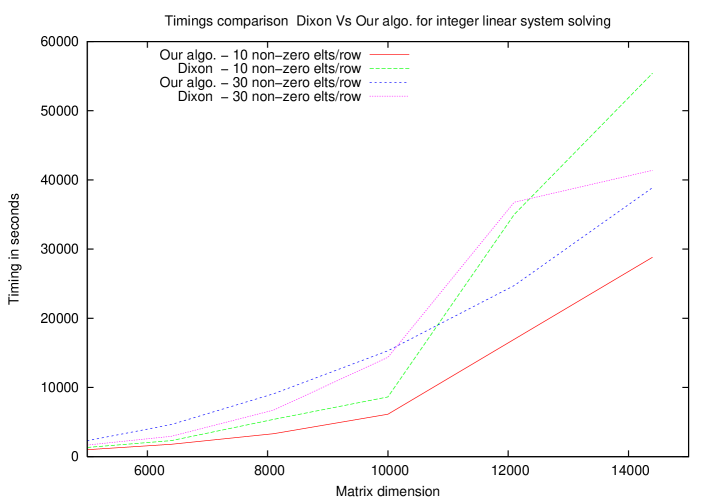
Figure 1: Comparing our algo. with Dixon’s algorithm (fixed sparsity) on a Itanium2, 1.3GHz

With $10$ non-zero element per row, our algorithm is always faster than Dixon’s and the gain tends to increase with matrix dimension. Its not exactly the same behaviour when matrices have $30$ non-zero element per row. For small matrices, Dixon still outperforms our algorithm. The crossover appears only after dimension $10\,000$. This phenomenon is explained by the fact that sparse matrix operations remain too costly compared to dense ones until matrix dimensions become sufficiently large that the overall asymptotic complexity plays a more important role.

This explanation is verified in Figure 2 where different sparsity percentages are used. The sparser the matrices are, the earlier the crossover appears. For instance, with a sparsity of $0.07\%$, our algorithm becomes more efficient than Dixon’s for matrices dimension greater than $1600$, while this is only true for dimension greater than $2500$ with a sparsity of $1\%$. Another phenomenon when examining matrices of a fixed percentage density is emphasized by the Figure 2. This is because Dixon’s algorithm again becomes the most efficient, in this case, when the matrices become large. This is explained by the variable sparsity which leads to a variable complexity. For a given sparsity, the larger the matrix dimensions the more non-zero entries per row, and the more costly our algorithm is. As an example, with $1\%$ of non zero element, the complexity is doubled from matrix dimension $n=3\,000$ to $n=6\,000$. As a consequence, the performances of our algorithm drop with matrix dimension in this particular case.

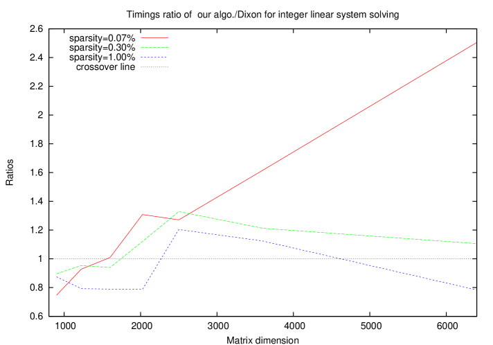
Figure 2: Gain of our algo. from Dixon’s algorithm (variable sparsity) on a Itanium2, 1.3GHz

4.3 The practical effect of different blocking factors

In order to achieve even better performance, one can try to use different block dimensions rather than the theoretical optimal $\sqrt{n}$. The Table 2 studies experimental blocking factors for matrices of dimension $n=10\,000$ and $n=20\,000$ with a fixed sparsity of $10$ non-zero elements per rows.

	n= 10 000
block size	80	125	200	400	500
timing	$7213$s	$5264$s	$4059$s	$\bf 3833$s	$4332$s
	n= 20 000
block size	125	160	200	500	800
timing	$44720$s	$35967$s	$30854$s	$\bf 28502$s	$37318$s

Table 2: Blocking factor impact (sparsity= 10 elts per row) on a Itanium2, 1.3GHz

One notices that the best experimental blocking factors are far from the optimal theoretical ones (e.g., the best blocking factor is $400$ when $n=10\,000$ whereas theoretically it is $100$). This behaviour is not surprising since the larger the blocking factor is, the fewer sparse matrix operations and the more dense matrix operations are performed. As we already noted earlier, operations are performed more efficiently when they are dense rather than sparse (the cache effect is of great importance in practice). However, as shown in Table 2, if the block dimensions become too large, the overall complexity of the algorithm increases and then becomes too important compared to Dixon’s. A function which should give a good approximation of the best practical blocking factor would be based on the practical efficiency of sparse matrix-vector product and dense matrix operations. Minimizing the complexity according to this efficiency would lead to a good candidate blocking factor. This could be done automatically at the beginning of the lifting by checking efficiency of sparse matrix-vector and dense operation for the given matrix.

Concluding remarks

We give a new approach to solving sparse linear algebra problems over the integers by using sparse or structured block projections. The algorithm we exhibit works well in practice. We demonstrate it on a collection of very large matrices and compare it against other state-of-the art algorithms. Its theoretical complexity is sub-cubic in terms of bit complexity, though it rests still on a conjecture which is not proven in the general case. We offer a rigorous treatment for a small blocking factor (2) and provide some support for the general construction.

The use of a block-Krylov-like algorithm allows us to link the problem of solving sparse integer linear systems to polynomial linear algebra, where we can benefit from both theoretical advances in this field and from the efficiency of dense linear algebra libraries. In particular, our experiments point out a general efficiency issue of sparse linear algebra: in practice, are (many) sparse operations as fast as (correspondingly fewer) dense operations? We have tried to show in this paper a negative answer to this question. Therefore, our approach to providing efficient implementations for sparse linear algebra problems has been to reduce most of the operations to dense linear algebra on a smaller scale. This work demonstrates an initial success for this approach (for integer matrices), and it certainly emphasizes the importance of well-designed (both theoretically and practically) sparse, symbolic linear algebra algorithms.

References

- [1] D. Cantor and E. Kaltofen. Fast multiplication of polynomials over arbitrary algebras. Acta Informatica, 28:693–701, 1991.
- [2] L. Chen, W. Eberly, E. Kaltofen, B. D. Saunders, W. J. Turner, and G. Villard. Efficient matrix preconditioners for black box linear algebra. Linear Algebra and its Applications, 343–344:119–146, 2002.
- [3] Z. Chen and A. Storjohann. A blas based c library for exact linear algebra on integer matrices. In ISSAC ’05: Proceedings of the 2005 international symposium on Symbolic and algebraic computation, pages 92–99, New York, NY, USA, 2005. ACM Press.
- [4] D. Coppersmith. Solving homogeneous linear equations over GF[2] via block Wiedemann algorithm. Mathematics of Computation, 62(205):333–350, Jan. 1994.
- [5] J. D. Dixon. Exact solution of linear equations using -adic expansions. Numerische Mathematik, 40:137–141, 1982.
- [6] J.-G. Dumas, T. Gautier, M. Giesbrecht, P. Giorgi, B. Hovinen, E. Kaltofen, B. D. Saunders, W. J. Turner, and G. Villard. LinBox: A generic library for exact linear algebra. In A. M. Cohen, X.-S. Gao, and N. Takayama, editors, Proceedings of the 2002 International Congress of Mathematical Software, Beijing, China, pages 40–50. World Scientific, Aug. 2002.
- [7] J.-G. Dumas, P. Giorgi, and C. Pernet. FFPACK: Finite field linear algebra package. In Gutierrez [12], pages 63–74.
- [8] W. Eberly, M. Giesbrecht, and G. Villard. On computing the determinant and Smith form of an integer matrix. In Proceedings of the 41st Annual Symposium on Foundations of Computer Science, page 675. IEEE Computer Society, 2000.
- [9] J. von zur Gathen and J. Gerhard. Modern Computer Algebra. Cambridge University Press, New York, USA, 1999.
- [10] M. Giesbrecht. Efficient parallel solution of sparse systems of linear diophantine equations. In Parallel Symbolic Computation (PASCO’97), pages 1–10, Maui, Hawaii, July 1997.
- [11] P. Giorgi, C.-P. Jeannerod, and G. Villard. On the complexity of polynomial matrix computations. In R. Sendra, editor, Proceedings of the 2003 International Symposium on Symbolic and Algebraic Computation, Philadelphia, Pennsylvania, USA, pages 135–142. ACM Press, New York, Aug. 2003.
- [12] J. Gutierrez, editor. ISSAC’2004. Proceedings of the 2004 International Symposium on Symbolic and Algebraic Computation, Santander, Spain. ACM Press, New York, July 2004.
- [13] G. H. Hardy and E. M. Wright. An Introduction to the Theory of Numbers. Oxford University Press, fifth edition, 1979.
- [14] E. Kaltofen. Analysis of Coppersmith’s block Wiedemann algorithm for the parallel solution of sparse linear systems. Mathematics of Computation, 64(210):777–806, Apr. 1995.
- [15] E. Kaltofen. Analysis of Coppersmith’s block Wiedemann algorithm for the parallel solution of sparse linear systems. Mathematics of Computation, 64(210):777–806, 1995.
- [16] E. Kaltofen and B. D. Saunders. On Wiedemann’s method of solving sparse linear systems. In Applied Algebra, Algebraic Algorithms and Error–Correcting Codes (AAECC ’91), volume 539 of LNCS, pages 29–38, Oct. 1991.
- [17] G. Labahn, D. K. Chio, and S. Cabay. The inverses of block hankel and block toeplitz matrices. SIAM J. Comput., 19(1):98–123, 1990.
- [18] R. T. Moenck and J. H. Carter. Approximate algorithms to derive exact solutions to systems of linear equations. In Proc. EUROSAM’79, volume 72 of Lecture Notes in Computer Science, pages 65–72, Berlin-Heidelberg-New York, 1979. Springer-Verlag.
- [19] T. Mulders and A. Storjohann. Diophantine linear system solving. In International Symposium on Symbolic and Algebraic Computation (ISSAC 99), pages 181–188, Vancouver, BC, Canada, July 1999.
- [20] T. Mulders and A. Storjohann. Certified dense linear system solving. Journal of Symbolic Computation, 37(4):485–510, 2004.
- [21] B. D. Saunders and Z. Wan. Smith normal form of dense integer matrices, fast algorithms into practice. In Gutierrez [12].
- [22] A. Storjohann. The shifted number system for fast linear algebra on integer matrices. Journal of Complexity, 21(4):609–650, 2005.
- [23] W. J. Turner. Black Box Linear Algebra with Linbox Library. PhD thesis, North Carolina State University, May 2002.
- [24] G. Villard. A study of Coppersmith’s block Wiedemann algorithm using matrix polynomials. Technical Report 975–IM, LMC/IMAG, Apr. 1997.
- [25] P. S. Wang. A -adic algorithm for univariate partial fractions. In Proceedings of the fourth ACM symposium on Symbolic and algebraic computation, pages 212–217. ACM Press, 1981.
- [26] D. H. Wiedemann. Solving sparse linear equations over finite fields. IEEE Transactions on Information Theory, 32(1):54–62, Jan. 1986.