Consensus Propagation

Abstract

We propose consensus propagation, an asynchronous distributed protocol for averaging numbers across a network. We establish convergence, characterize the convergence rate for regular graphs, and demonstrate that the protocol exhibits better scaling properties than pairwise averaging, an alternative that has received much recent attention. Consensus propagation can be viewed as a special case of belief propagation, and our results contribute to the belief propagation literature. In particular, beyond singly-connected graphs, there are very few classes of relevant problems for which belief propagation is known to converge.

I Introduction

Consider a network of $n$ nodes in which the $i$th node observes a real number $y_{i}\in\mathbb{R}$ and aims to compute the average $\bar{y}=\sum_{i=1}^{n}y_{i}/n$. The design of scalable distributed protocols for this purpose has received much recent attention and is motivated by a variety of potential needs. In both wireless sensor and peer-to-peer networks, for example, there is interest in simple protocols for computing aggregate statistics (see, e.g. [1, 2, 3, 4, 5, 6, 7]), and averaging enables computation of several important ones. Further, averaging serves as a primitive in the design of more sophisticated distributed information processing algorithms. For example, a maximum likelihood estimate can be produced by an averaging protocol if each node’s observations are linear in variables of interest and noise is Gaussian [8]. [9] considers an averaging problem with applications to load balancing and clock synchronization. As another example, averaging protocols are central to policy-gradient-based methods for distributed optimization of network performance [10].

In this paper we propose and analyze a new protocol – consensus propagation – for distributed averaging. The protocol can operate asynchronously and requires only simple iterative computations at individual nodes and communication of parsimonious messages between neighbors. There is no central hub that aggregates information. Each node only needs to be aware of its neighbors – no further information about the network topology is required. There is no need for construction of a specially-structured overlay network such as a spanning tree. It is worth discussing two previously proposed and well-studied protocols that also exhibit these features:

1. (probabilistic counting) This protocol is based on ideas from [11] for counting distinct elements of a database and in [12] was adapted to produce a protocol for averaging. The outcome is random, with variance that becomes arbitrarily small as the number of nodes grows. However, for moderate numbers of nodes, say tens of thousands, high variance makes the protocol impractical. The protocol can be repeated in parallel and results combined in order to reduce variance, but this leads to onerous memory and communication requirements. Convergence time of the protocol is analyzed in [13].

2. (pairwise averaging) In this protocol, each node maintains its current estimate of the average, and each time a pair of nodes communicate, they revise their estimates to both take on the mean of their previous estimates. Convergence of this protocol in a very general model of asynchronous computation and communication was established in [14], and there has been significant follow-on work, a recent sample of which is [15]. Recent work [16, 17] has studied the convergence rate and its dependence on network topology and how pairs of nodes are sampled. Here, sampling is governed by a certain doubly stochastic matrix, and the convergence rate is characterized by its second-largest eigenvalue.

In terms of convergence rate, probabilistic counting dominates both pairwise averaging and consensus propagation in the asymptotic regime. However, consensus propagation and pairwise averaging are likely to be more effective in moderately-sized networks (up to hundreds of thousands or perhaps even millions of nodes). Further, these two protocols are both naturally studied as iterative matrix algorithms. As such, pairwise averaging will serve as a baseline to which we will compare consensus propagation.

Consensus propagation is a simple algorithm with an intuitive interpretation. It can also be viewed as an asynchronous distributed version of belief propagation as applied to approximation of conditional distributions in a Gaussian Markov random field. When the network of interest is singly-connected, prior results about belief propagation imply convergence of consensus propagation. However, in most cases of interest, the network is not singly-connected and prior results have little to say about convergence. In particular, Gaussian belief propagation on a graph with cycles is not guaranteed to converge, as demonstrated by numerical examples in [18].

In fact, there are very few relevant cases where belief propagation on a graph with cycles is known to converge. Some fairly general sufficient conditions have been established [19, 20, 21, 22], but these conditions are abstract and it is difficult to identify interesting classes of problems that meet them. One simple case where belief propagation is guaranteed to converge is when the graph has only a single cycle and variables have finite support [23, 24, 25]. In its use for decoding low-density parity-check codes, though convergence guarantees have not been made, [26] establishes desirable properties of iterates, which hold with high probability. Recent work proposes the use of belief propagation to solve maximum-weight matching problems and proves convergence in that context [27]. In the Gaussian case, [18, 28] provide sufficient conditions for convergence, but these conditions are difficult to interpret and do not capture situations that correspond to consensus propagation. Since this paper was submitted for publication, a general class of results has been developed for the convergence of Gaussian belief propagation [29, 30]. These results can be viewed as a generalization of the convergence results in this paper. However, they do not address the issue of rate of convergence.

With this background, let us discuss the primary contributions of this paper:

1. We propose consensus propagation, a new asynchronous distributed protocol for averaging.

2. We prove that consensus propagation converges even when executed asynchronously. Since there are so few classes of relevant problems for which belief propagation is known to converge, even with synchronous execution, this is surprising.

3. We characterize the convergence time in regular graphs of the synchronous version of consensus propagation in terms of the the mixing time of a certain Markov chain over edges of the graph.

4. We explain why the convergence time of consensus propagation scales more gracefully with the number of nodes than does that of pairwise averaging, and for certain classes of graphs, we quantify the improvement.

It is worth mentioning a recent and related line of research on the use of belief propagation as an asynchronous distributed protocol to arrive at consensus among nodes in a network, when each node makes a conditionally independent observation of the class of an object and would like to know the most probable class based on all observations [31]. The authors establish that belief propagation converges and provides each node with the most probable class when the network is a tree or a regular graph. They further show that for a certain class of random graphs, the result holds in an asymptotic sense as the number of nodes grows. To deal with general connected graphs, the authors offer a more complex protocol with convergence guarantees. It is interesting to note that this classification problem can be reduced to one of averaging. In particular, if each node starts out with the conditional probability of each class given its own observation and the network carries out a protocol to compute the average log-probability for each class, each node obtains the conditional probabilities given all observations. Hence, consensus propagation also solves this classification problem.

II Algorithm

Consider a connected undirected graph $(V,E)$ with $V=\{1,\ldots,n\}$. For each node $i\in V$, let $N(i)=\{j\ |\ (i,j)\in E\}$ be the set of neighbors of $i$. Let $\vec{E}\subseteq V\times V$ be a set consisting of two directed edges $\{i,j\}$ and $\{j,i\}$ per undirected edge $(i,j)\in E$. (In general, we will use braces for directed edges and parentheses for undirected edges.)

Each node $i\in V$ is assigned a number $y_{i}\in\mathbb{R}$. The goal is for each node to obtain an estimate of $\bar{y}=\sum_{i\in V}y_{i}/n$ through an asynchronous distributed protocol in which each node carries out simple computations and communicates parsimonious messages to its neighbors.

We propose consensus propagation as an approach to the aforementioned problem. In this protocol, if a node $i$ communicates to a neighbor $j$ at time $t$, it transmits a message consisting of two numerical values. Let $\mu^{(t)}_{ij}\in\mathbb{R}$ and $K^{(t)}_{ij}\in\mathbb{R}_{+}$ denote the values associated with the most recently transmitted message from $i$ to $j$ at or before time $t$. At each time $t$, node $i$ has stored in memory the most recent message from each neighbor: $\{\mu^{(t)}_{ui},K^{(t)}_{ui}\ |\ u\in N(i)\}$. If, at time $t+1$, node $i$ chooses to communicate with a neighboring node $j\in N(i)$, it constructs a new message that is a function of the set of most recent messages $\{\mu^{(t)}_{ui},K^{(t)}_{ui}\ |\ u\in N(i)\setminus j\}$ received from neighbors other than $j$. The initial values in memory before receiving any messages are arbitrary.

In order to illustrate how the parameter vectors $\mu^{(t)}$ and $K^{(t)}$ evolve, we will first describe a special case of the consensus propagation algorithm that is particularly intuitive. Then, we will describe the general algorithm and its relationship to belief propagation.

II-A Intuitive Interpretation

Consider the special case of a singly-connected graph. That is, a connected graph where there are no loops present (a tree). Assume, for the moment, that at every point in time, every pair of connected nodes communicates. As illustrated in Fig. 1, for any edge $\{i,j\}\in\vec{E}$, there is a set $S_{ij}\subset V$ of nodes, with $i\in S_{ij}$, that can transmit information to $S_{ji}=V\setminus S_{ij}$, with $j\in S_{ji}$, only through $\{i,j\}$. In order for nodes in $S_{ji}$ to compute $\overline{y}$, they must at least be provided with the average $\mu^{*}_{ij}$ among observations at nodes in $S_{ij}$ and the cardinality $K^{*}_{ij}=|S_{ij}|$. Similarly, in order for nodes in $S_{ij}$ to compute $\overline{y}$, they must at least be provided with the average $\mu^{*}_{ji}$ among observations at nodes in $S_{ji}$ and the cardinality $K^{*}_{ji}=|S_{ji}|$. These values must be communicated through the link $\{j,i\}$.

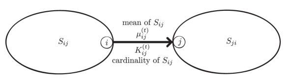
Figure 1: Interpretation of messages in a singly connected graph with $\beta=\infty$.

The messages $\mu^{(t)}_{ij}$ and $K^{(t)}_{ij}$, transmitted from node $i$ to node $j$, can be viewed as iterative estimates of the quantities $\mu^{*}_{ij}$ and $K^{*}_{ij}$. They evolve according to

$$\mu^{(t)}_{ij} =\frac{y_{i}+\sum_{u\in N(i)\setminus j}K^{(t-1)}_{ui}\mu^{(t-1)}_{ui}}{1+\sum_{u\in N(i)\setminus j}K^{(t-1)}_{ui}}, \forall\ \{i,j\}\in\vec{E},$$ (1a)

$$K^{(t)}_{ij} =1+\sum_{u\in N(i)\setminus j}K^{(t-1)}_{ui}, \forall\ \{i,j\}\in\vec{E}.$$ (1b)

At each time $t$, each node $i$ computes an estimate of the global average $\bar{y}$ according to

$$x^{(t)}_{i}=\frac{y_{i}+\sum_{u\in N(i)}K^{(t)}_{ui}\mu^{(t)}_{ui}}{1+\sum_{u\in N(i)}K^{(t)}_{ui}}.$$

Assume that the algorithm is initialized with $K^{(0)}=0$. A simple inductive argument shows that at each time $t\geq 1$, $\mu_{ij}^{(t)}$ is the average among observations at the nodes in the set $S_{ij}$ that are at a distance less than or equal to $t$ from node $i$. Furthermore, $K^{(t)}_{ij}$ is the cardinality of this collection of nodes. Since any node in $S_{ij}$ is at a distance from node $i$ that it at most the diameter of the graph, if $t$ is greater that the diameter of the graph, we have $K^{(t)}=K^{*}$ and $\mu^{(t)}=\mu^{*}$. Thus, for any $i\in V$, and $t$ sufficiently large,

$$x^{(t)}_{i}=\frac{y_{i}+\sum_{u\in N(i)}K^{*}_{ui}\mu^{*}_{ui}}{1+\sum_{u\in N(i)}K^{*}_{ui}}=\overline{y}.$$

So, $x_{i}^{(t)}$ converges to the global average $\overline{y}$. Further, this simple algorithm converges in as short a time as is possible, since the diameter of the graph is the minimum amount of time for the two most distance nodes to communicate.

Now, suppose that the graph has cycles. For any directed edge $\{i,j\}\in\vec{E}$ that is part of a cycle, $K^{(t)}_{ij}\rightarrow\infty$. Hence, the algorithm does not converge. A heuristic fix might be to compose the iteration (1b) with one that attenuates:

$$\tilde{K}^{(t)}_{ij} \leftarrow 1+\sum_{u\in N(i)\setminus j}K^{(t-1)}_{ui},$$

$$K^{(t)}_{ij} \leftarrow\frac{\tilde{K}^{(t)}_{ij}}{1+\tilde{K}^{(t)}_{ij}/(\beta Q_{ij})}.$$

Here, $Q_{ij}>0$ and $\beta>0$ are positive constants. We can view the unattenuated algorithm as setting $\beta=\infty$. In the attenuated algorithm, the message is essentially unaffected when $\tilde{K}^{(t)}_{ij}/(\beta Q_{ij})$ is small but becomes increasingly attenuated as $\tilde{K}^{(t)}_{ij}$ grows. This is exactly the kind of attenuation carried out by consensus propagation. Understanding why this kind of attenuation leads to desirable results is a subject of our analysis.

II-B General Algorithm

Consensus propagation is parameterized by a scalar $\beta>0$ and a non-negative matrix $Q\in\mathbb{R}_{+}^{n\times n}$ with $Q_{ij}>0$ if and only if $i\neq j$ and $(i,j)\in E$. For each $\{i,j\}\in\vec{E}$, it is useful to define the following three functions:

$${\cal F}_{ij}(K) =\frac{1+\sum_{u\in N(i)\setminus j}K_{ui}}{1+\frac{1}{\beta Q_{ij}}\left(1+\sum_{u\in N(i)\setminus j}K_{ui}\right)},$$ (2a)

$${\cal G}_{ij}(\mu,K) =\frac{y_{i}+\sum_{u\in N(i)\setminus j}K_{ui}\mu_{ui}}{1+\sum_{u\in N(i)\setminus j}K_{ui}},$$ (2b)

$${\cal X}_{i}(\mu,K) =\frac{y_{i}+\sum_{u\in N(i)}K_{ui}\mu_{ui}}{1+\sum_{u\in N(i)}K_{ui}}.$$ (2c)

For each $t$, denote by $U_{t}\subseteq\vec{E}$ the set of directed edges along which messages are transmitted at time $t$. Consensus propagation is presented below as Algorithm 1.

Algorithm 1 Consensus propagation.

1:  for time $t=1$ to $\infty$ do

2:     for all $\{i,j\}\in U_{t}$ do

3:        $K_{ij}^{(t)}\leftarrow{\cal F}_{ij}(K^{(t-1)})$

4:        $\mu_{ij}^{(t)}\leftarrow{\cal G}_{ij}(\mu^{(t-1)},K^{(t-1)})$

5:     end for

6:     for all $\{i,j\}\notin U_{t}$ do

7:        $K_{ij}^{(t)}\leftarrow K_{ij}^{(t-1)}$

8:        $\mu_{ij}^{(t)}\leftarrow\mu_{ij}^{(t-1)}$

9:     end for

10:     $x^{(t)}\leftarrow{\cal X}(\mu^{(t)},K^{(t)})$

11:  end for

Consensus propagation is a distributed protocol because computations at each node require only information that is locally available. In particular, the messages $K^{(t)}_{ij}={\cal F}_{ij}(K^{(t-1)})$ and $\mu^{(t)}_{ij}={\cal G}_{ij}(\mu^{(t-1)},K^{(t-1)})$ transmitted from node $i$ to node $j$ depend only on $\{\mu^{(t-1)}_{ui},K^{(t-1)}_{ui}\ |\ u\in N(i)\}$, which node $i$ has stored in memory. Similarly, $x_{i}^{(t)}$, which serves as an estimate of $\overline{y}$, depends only on $\{\mu^{(t)}_{ui},K^{(t)}_{ui}\ |\ u\in N(i)\}$.

Consensus propagation is an asynchronous protocol because only a subset of the potential messages are transmitted at each time. Our convergence analysis can also be extended to accommodate more general models of asynchronism that involve communication delays, as those presented in [32].

In our study of convergence time, we will focus on the synchronous version of consensus propagation. This is where $U_{t}=\vec{E}$ for all $t$. Note that synchronous consensus propagation is defined by:

$$K^{(t)} ={\cal F}(K^{(t-1)}),$$ (3a)

$$\mu^{(t)} ={\cal G}(\mu^{(t-1)},K^{(t-1)}),$$ (3b)

$$x^{(t)} ={\cal X}(\mu^{(t-1)},K^{(t-1)}).$$ (3c)

II-C Relation to Belief Propagation

Consensus propagation can also be viewed as a special case of belief propagation. In this context, belief propagation is used to approximate the marginal distributions of a vector $x\in\mathbb{R}^{n}$ conditioned on the observations $y\in\mathbb{R}^{n}$. The mode of each of the marginal distributions approximates $\overline{y}$.

Take the prior distribution over $(x,y)$ to be the normalized product of potential functions $\{\psi_{i}(\cdot)\ |\ i\in V\}$ and compatibility functions $\{\psi^{\beta}_{ij}(\cdot)\ |\ (i,j)\in E\}$, given by

$$\psi_{i}(x_{i}) =\exp(-(x_{i}-y_{i})^{2}),$$

$$\psi^{\beta}_{ij}(x_{i},x_{j}) =\exp(-\beta Q_{ij}(x_{i}-x_{j})^{2}),$$

where $Q_{ij}>0$, for each edge $(i,j)\in E$, and $\beta>0$ are constants. Note that $\beta$ can be viewed as an inverse temperature parameter; as $\beta$ increases, components of $x$ associated with adjacent nodes become increasingly correlated.

Let $\Gamma$ be a positive semidefinite symmetric matrix such that

$$x^{\top}\Gamma x=\sum_{(i,j)\in E}Q_{ij}(x_{i}-x_{j})^{2}.$$

Note that when $Q_{ij}=1$, for all edges $(i,j)\in E$, $\Gamma$ is the graph Laplacian. Given the vector $y$ of observations, the conditional density of $x$ is

$$\begin{split}p^{\beta}(x)&\propto\prod_{i\in V}\psi_{i}(x_{i})\prod_{(i,j)\in E}\psi^{\beta}_{ij}(x_{i},x_{j})\\ &=\exp\left(-\|x-y\|^{2}_{2}-\beta x^{\top}\Gamma x\right).\end{split}$$

Let $x^{\beta}$ denote the mode (maximizer) of $p^{\beta}(\cdot)$. Since the distribution is Gaussian, each component $x_{i}^{\beta}$ is also the mode of the corresponding marginal distribution. Note that $x^{\beta}$ it is the unique solution to the positive definite quadratic program

$$\mathop{\mbox{\rm minimize}}\limits_{x}\quad\|x-y\|^{2}_{2}+\beta x^{\top}\Gamma x.$$ (4)

The following theorem relates $x^{\beta}$ to the mean value $\bar{y}$.

Theorem 1

$\sum_{i}x^{\beta}_{i}/n=\bar{y}$ and $\lim_{\beta\uparrow\infty}x^{\beta}_{i}=\bar{y}$, for all $i\in V$.

Proof:

The first order conditions for optimality imply $(I+\beta\Gamma)x^{\beta}=y$. If we set ${\bf 1}=(1,\ldots,1)^{\top}\in\mathbb{R}^{n}$, we have $\Gamma{\bf 1}=0$, hence ${\bf 1}^{\top}x^{\beta}/n={\bf 1}^{\top}y/n=\bar{y}$. Let $U$ be an orthogonal matrix and $D$ a diagonal matrix that form a spectral decomposition of $\Gamma$, that is $\Gamma=U^{\top}DU$. Then, we have $x^{\beta}=U^{\top}(I+\beta D)^{-1}Uy$. It is clear that $\Gamma$ has eigenvalue 0 with multiplicity 1 and corresponding normalized eigenvector ${\bf 1}/\sqrt{n}$, and all other eigenvalues $d_{2},\ldots,d_{n}$ of $\Gamma$ are positive. Then, if $D=\mathop{\mbox{\rm diag}}(0,d_{2},\ldots,d_{n})$,

$$\begin{split}\@ADDCLASS{ltx_eqn_lefteqn}$\displaystyle\lim_{\beta\rightarrow\infty}x^{\beta}$\mbox{}\hfil&\\ &=\lim_{\beta\rightarrow\infty}U^{\top}\mathop{\mbox{\rm diag}}(1,1/(1+\beta d_{2}),\ldots,1/(1+\beta d_{n}))Uy\\ &={\bf 1}{\bf 1}^{\top}y/n.\end{split}$$

∎

The above theorem suggests that if $\beta$ is sufficiently large, then each component $x^{\beta}_{i}$ can be used as an estimate of $\bar{y}$.

In belief propagation, messages are passed along edges of a Markov random field. In our case, because of the structure of the distribution $p^{\beta}(\cdot)$, the relevant Markov random field has the same topology as the graph $(V,E)$. The message $M^{(t)}_{ij}(\cdot)$ passed from node $i$ to node $j$ at time $t$ is a distribution on the variable $x_{j}$. Node $i$ computes this message using incoming messages from other nodes as defined by the update equation

$$M^{(t)}_{ij}(x_{j})=\kappa\int\psi_{ij}(x^{\prime}_{i},x_{j})\psi_{i}(x^{\prime}_{i})\prod_{u\in N(i)\setminus j}M^{(t-1)}_{ui}(x^{\prime}_{i})\ dx^{\prime}_{i}.$$ (5)

Here, $\kappa$ is a normalizing constant. Since our underlying distribution $p^{\beta}(\cdot)$ is Gaussian, it is natural to consider messages which are Gaussian distributions. In particular, let $(\mu^{(t)}_{ij},K^{(t)}_{ij})\in\mathbb{R}\times\mathbb{R}_{+}$ parameterize Gaussian message $M^{(t)}_{ij}(\cdot)$ according to

$$M^{(t)}_{ij}(x_{j})\propto\exp\left(-K^{(t)}_{ij}(x_{j}-\mu^{(t)}_{ij})^{2}\right).$$

Then, (5) is equivalent to the synchronous consensus propagation iterations for $K^{(t)}$ and $\mu^{(t)}$.

The sequence of densities

$$\begin{split}p^{(t)}_{j}(x_{j})&\propto\psi_{j}(x_{j})\prod_{i\in N(j)}M^{(t)}_{ij}(x_{j})\\ &=\exp\left(-(x_{j}-y_{j})^{2}-\sum_{i\in N(j)}K^{(t)}_{ij}(x_{j}-\mu^{(t)}_{ij})^{2}\right),\end{split}$$

is meant to converge to an approximation of the marginal conditional distribution of $x_{j}$. As such, an approximation to $x^{\beta}_{j}$ is given by maximizing $p^{(t)}_{j}(\cdot)$. It is easy to show that, the maximum is attained by $x^{(t)}_{j}={\cal X}_{j}(\mu^{(t)},K^{(t)})$. With this and aforementioned correspondences, we have shown that consensus propagation is a special case of belief propagation, and more specifically, Gaussian belief propagation.

Readers familiar with belief propagation will notice that in the derivation above we have used the sum-product form of the algorithm. In this case, since the underlying distribution is Gaussian, the max-product form yields equivalent iterations.

II-D Relation to Prior Results

In light of the fact that consensus propagation is a special case of Gaussian belief propagation, it is natural to ask what prior results on belief propagation — Gaussian or more broadly — have to say in this context. Results from [28, 18, 33] establish that, in the absence of degeneracy, Gaussian belief propagation has a unique fixed point and that the mode of this fixed point is unbiased. The issue of convergence, however, is largely poorly understood. As observed numerically in [18], Gaussian belief propagation can diverge, even in the absence of degeneracy. Abstract sufficient conditions for convergence that have been developed in [28, 18] are difficult to verify in the consensus propagation case.

III Convergence

As we have discussed, Gaussian belief propagation can diverge, even when the graph has a single cycle. One might expect the same from consensus propagation. However, the following theorem establishes convergence.

Theorem 2

The following hold:

• There exist unique vectors $(\mu^{\beta},K^{\beta})$ such that $K^{\beta}={\cal F}(K^{\beta})$ and $\mu^{\beta}={\cal G}(\mu^{\beta},K^{\beta})$.

• Suppose that each directed edge $\{i,j\}$ appears infinitely often in the sequence of communication sets $\{U_{t}\}$. Then, independent of the initial condition $(\mu^{(0)},K^{(0)})$,

  $$\lim_{t\rightarrow\infty}K^{(t)}=K^{\beta},\quad\text{and}\quad\lim_{t\rightarrow\infty}\mu^{(t)}=\mu^{\beta}.$$

• Given $(\mu^{\beta},K^{\beta})$, if $x^{\beta}={\cal X}(\mu^{\beta},K^{\beta})$, then $x^{\beta}$ is the mode of the distribution $p^{\beta}(\cdot)$.

Note that the condition on the communication sets in Theorem 2(ii) corresponds to total asynchronism in the language of [32]. This is a weak assumption which ensures only that every component of $\mu^{(t)}$ and $K^{(t)}$ is updated infinitely often.

The proof of this theorem is deferred until the appendix, but it rests on two ideas. First, notice that, according to the update equation (2a), $K^{(t)}$ evolves independently of $\mu^{(t)}$. Hence, we analyze $K^{(t)}$ first. Following the work in [18], we prove that the functions $\{{\cal F}_{ij}(\cdot)\}$ are monotonic. This property is used to establish convergence to a unique fixed point. Next, we analyze $\mu^{(t)}$ assuming that $K^{(t)}$ has already converged. Given fixed $K$, the update equations for $\mu^{(t)}$ are linear, and we establish that they induce a contraction with respect to the maximum norm. This allows us to establish existence of a fixed point and both synchronous and asynchronous convergence.

IV Convergence Time for Regular Graphs

In this section, we will study the convergence time of synchronous consensus propagation. For $\epsilon>0$, we will say that an estimate $\tilde{x}$ of $\bar{y}$ is $\epsilon$-accurate if

$$\|\tilde{x}-\bar{y}{\bf 1}\|_{2,n}\leq\epsilon.$$ (6)

Here, for integer $m$, we set $\|\cdot\|_{2,m}$ to be the norm on $\mathbb{R}^{m}$ defined by $\|x\|_{2,m}=\|x\|_{2}/\sqrt{m}$. We are interested in the number of iterations required to obtain an $\epsilon$-accurate estimate of the mean $\bar{y}$.

Note that we are primarily interested in how the performance of consensus propagation behaves over a series of problem instances as we scale the size of the graph. Since our measure of error (6) is absolute, we require that the set of values $\{y_{i}\}$ lie in some bounded set. Without loss of generality, we will take $y_{i}\in[0,1]$, for all $i\in V$.

IV-A The Case of Regular Graphs

We will restrict our analysis of convergence time to cases where $(V,E)$ is a $d$-regular graph, for $d\geq 2$. Extension of our analysis to broader classes of graphs remains an open issue. We will also make simplifying assumptions that $Q_{ij}=1$, $\mu^{(0)}_{ij}=y_{i}$, and $K^{(0)}=[k_{0}]_{ij}$ for some scalar $k_{0}\geq 0$.

In this restricted setting, the subspace of constant $K$ vectors is invariant under ${\cal F}$. This implies that there is some scalar $k^{\beta}>0$ so that $K^{\beta}=[k^{\beta}]_{ij}$. This $k^{\beta}$ is the unique solution to the fixed point equation

$$k^{\beta}=\frac{1+(d-1)k^{\beta}}{1+(1+(d-1)k^{\beta})/\beta}.$$ (7)

Given a uniform initial condition $K^{(0)}=[k_{0}]_{ij}$, we can study the sequence of iterates $\{K^{(t)}\}$ by examining the scalar sequence $\{k_{t}\}$, defined by

$$k_{t}=\frac{1+(d-1)k_{t-1}}{1+(1+(d-1)k_{t-1})/\beta}.$$ (8)

In particular, we have $K^{(t)}=[k_{t}]_{ij}$, for all $t\geq 0$.

Similarly, in this setting, the equations for the evolution of $\mu^{(t)}$ take the special form

$$\begin{split}\mu^{(t)}_{ij}&=\frac{y_{i}}{1+(d-1)k_{t-1}}\\ &\quad+\>\left(1-\frac{1}{1+(d-1)k_{t-1}}\right)\sum_{u\in N(i)\setminus j}\frac{\mu^{(t-1)}_{ui}}{d-1}.\end{split}$$

Defining $\gamma_{t}=1/(1+(d-1)k_{t})$, we have, in vector form,

$$\mu^{(t)}=\gamma_{t-1}\hat{y}+(1-\gamma_{t-1})\hat{P}\mu^{(t-1)},$$ (9)

where $\hat{y}\in\mathbb{R}^{nd}$ is a vector with $\hat{y}_{ij}=y_{i}$ and $\hat{P}\in\mathbb{R}_{+}^{nd\times nd}$ is a doubly stochastic matrix. The matrix $\hat{P}$ corresponds to a Markov chain on the set of directed edges $\vec{E}$. In this chain, a directed edge $\{i,j\}$ transitions to a directed edge $\{u,i\}$ with $u\in N(i)\setminus j$, with equal probability assigned to each such edge. As in (3), we associate each $\mu^{(t)}$ with an estimate $x^{(t)}$ of $x^{\beta}$ according to

$$x^{(t)}=\frac{1}{1+dk^{\beta}}y+\frac{dk^{\beta}}{1+dk^{\beta}}A\mu^{(t)},$$

where $A\in\mathbb{R}_{+}^{n\times nd}$ is a matrix defined by $(A\mu)_{j}=\sum_{i\in N(j)}\mu_{ij}/d$.

IV-B The Cesàro Mixing Time

The update equation (9) suggests that the convergence of $\mu^{(t)}$ is intimately tied to a notion of mixing time associated with $\hat{P}$. Let $\hat{P}^{\star}$ be the Cesàro limit

$$\hat{P}^{\star}=\lim_{t\rightarrow\infty}\sum_{\tau=0}^{t-1}\hat{P}^{\tau}/t.$$

Define the Cesàro mixing time $\tau^{\star}$ by

$$\tau^{\star}=\sup_{t\geq 0}\left\|\sum_{\tau=0}^{t}(\hat{P}^{\tau}-\hat{P}^{\star})\right\|_{2,nd}.$$

Here, $\|\cdot\|_{2,nd}$ is the matrix norm induced by the corresponding vector norm $\|\cdot\|_{2,nd}$. Since $\hat{P}$ is a stochastic matrix, $\hat{P}^{\star}$ is well-defined and $\tau^{\star}<\infty$. Note that, in the case where $\hat{P}$ is aperiodic, irreducible, and symmetric, $\tau^{\star}$ corresponds to the traditional definition of mixing time: the inverse of the spectral gap of $\hat{P}$.

IV-C Bounds on the Convergence Time

Let $\gamma^{\beta}=\lim_{t\uparrow\infty}\gamma_{t}=1/(1+(d-1)k^{\beta})$. With an initial condition $k_{0}=k^{\beta}$, the update equation for $\mu^{(t)}$ becomes

$$\mu^{(t)}=\gamma^{\beta}\hat{y}+(1-\gamma^{\beta})\hat{P}\mu^{(t-1)}.$$

Since $\gamma^{\beta}\in(0,1)$, this iteration is a contraction mapping, with contraction factor $1-\gamma^{\beta}$. It is easy to show that $\gamma^{\beta}$ is monotonically decreasing in $\beta$, and as such, large values of $\beta$ are likely to result in slower convergence. On the other hand, Theorem 1 suggests that large values of $\beta$ are required to obtain accurate estimates of $\bar{y}$. To balance these conflicting issues, $\beta$ must be appropriately chosen.

A time $t^{*}$ is said to be an $\epsilon$-convergence time if estimates $x^{(t)}$ are $\epsilon$-accurate for all $t\geq t^{*}$. The following theorem, whose proof is deferred until the appendix, establishes a bound on the $\epsilon$-convergence time of synchronous consensus propagation given appropriately chosen $\beta$, as a function of $\epsilon$ and $\tau^{\star}$.

Theorem 3

Suppose $k_{0}\leq k^{\beta}$. If $d=2$ there exists a $\beta=\Theta((\tau^{\star}/\epsilon)^{2})$ and if $d>2$ there exists a $\beta=\Theta(\tau^{\star}/\epsilon)$ such that some $t^{*}=O((\tau^{\star}/\epsilon)\log(\tau^{\star}/\epsilon))$ is an $\epsilon$-convergence time.

In the above theorem, $k_{0}$ is initialized arbitrarily so long as $k_{0}\leq k^{\beta}$. Typically, one might set $k_{0}=0$ to guarantee this. Another case of particular interest is when $k_{0}=k^{\beta}$, so that $k_{t}=k^{\beta}$ for all $t\geq 0$. In this case, the following theorem, whose proof is deferred until the appendix, offers a better convergence time bound than Theorem 3.

Theorem 4

Suppose $k_{0}=k^{\beta}$. If $d=2$ there exists a $\beta=\Theta((\tau^{\star}/\epsilon)^{2})$ and if $d>2$ there exists a $\beta=\Theta(\tau^{\star}/\epsilon)$ such that some $t^{*}=O((\tau^{\star}/\epsilon)\log(1/\epsilon))$ is an $\epsilon$-convergence time.

Theorems 3 and 4 suggest that initializing with $k_{0}=k^{\beta}$ leads to an improvement in convergence time. However, in our computational experience, we have found that an initial condition of $k_{0}=0$ consistently results in faster convergence than $k_{0}=k^{\beta}$. Hence, we suspect that a convergence time bound of $O((\tau^{\star}/\epsilon)\log(1/\epsilon))$ also holds for the case of $k_{0}=0$. Proving this remains an open issue.

IV-D Adaptive Mixing Time Search

The choice of $\beta$ is critical in that it determines both convergence time and ultimate accuracy. This raises the question of how to choose $\beta$ for a particular graph. The choices posited in Theorems 3 and 4 require knowledge of $\tau^{\star}$, which may be both difficult to compute and also requires knowledge of the graph topology. This counteracts our purpose of developing a distributed protocol.

In order to address this concern, consider Algorithm 2, which is designed for the case of $d>2$. It uses a doubling sequence of guesses $\tilde{\tau}$ for the Cesáro mixing time $\tau^{\star}$. Each guess leads to a choice of $\beta$ and a number of iterations $t^{*}$. Note that the algorithm takes $\epsilon>0$ as input.

Algorithm 2 Synchronous consensus propagation with adaptive mixing time search.

1:  $K^{(0)}\leftarrow 0$, $\mu^{(0)}\leftarrow\hat{y}$, $t\leftarrow 0$

2:  for $\ell=0$ to $\infty$ do

3:     $\tilde{\tau}\leftarrow 2^{\ell}$

4:     Set $\beta$ and $t^{*}$ as indicated by Theorem 3, assuming $\tau^{\star}=\tilde{\tau}$

5:     for $s=1$ to $t^{*}$ do

6:        $\mu^{(t)}\leftarrow{\cal G}(\mu^{(t-1)},K^{(t-1)})$, $K^{(t)}\leftarrow{\cal F}(K^{(t)})$

7:        $t\leftarrow t+1$

8:     end for

9:  end for

Consider applying this procedure to a $d$-regular graph with fixed $d>2$ but topology otherwise unspecified. It follows from Theorem 3 that this procedure has an $\epsilon$-convergence time of $O((\tau^{\star}/\epsilon)\log(\tau^{\star}/\epsilon))$. An entirely analogous algorithm can be designed for the case of $d=2$.

We expect that many variations of this procedure can be made effective. Asynchronous versions would involve each node adapting a local estimate of the mixing time.

V Comparison with Pairwise Averaging

Using the results of Section IV, we can compare the performance of consensus propagation to that of pairwise averaging. Pairwise averaging is usually defined in an asynchronous setting, but there is a synchronous counterpart which works as follows. Consider a doubly stochastic symmetric matrix $P\in\mathbb{R}^{n\times n}$ such that $P_{ij}=0$ if $i\neq j$ and $(i,j)\notin E$. Evolve estimates according to $x^{(t)}=Px^{(t-1)}$, initialized with $x^{(0)}=y$. Here, at each time $t$, a node $i$ is computing a new estimate $y^{(t)}_{i}$ which is an average of the estimates at node $i$ and its neighbors during the previous time-step. If the matrix $P$ is aperiodic and irreducible, then $x^{(t)}=P^{t}y\rightarrow\bar{y}{\bf 1}$ as $t\uparrow\infty$.

In the case of a singly-connected graph, synchronous consensus propagation converges exactly in a number of iterations equal to the diameter of the graph. Moreover, when $\beta=\infty$, this convergence is to the exact mean, as discussed in Section II-A. This is the best one can hope for under any algorithm, since the diameter is the minimum amount of time required for a message to travel between the two most distant nodes. On the other hand, for a fixed accuracy $\epsilon$, the worst-case number of iterations required by synchronous pairwise averaging on a singly-connected graph scales at least quadratically in the diameter [34].

The rate of convergence of synchronous pairwise averaging is governed by the relation $\|x^{(t)}-\bar{y}{\bf 1}\|_{2,n}\leq\lambda_{2}^{t}$, where $\lambda_{2}$ is the second largest eigenvalue of $P$. Let $\tau_{2}=1/\log(1/\lambda_{2})$, and call it the mixing time of $P$. In order to guarantee $\epsilon$-accuracy (independent of $y$), $t>\tau_{2}\log(1/\epsilon)$ suffices and $t=\Omega(\tau_{2}\log(1/\epsilon))$ is required.

Consider $d$-regular graphs and fix a desired error tolerance $\epsilon$. The number of iterations required by consensus propagation is $\Theta(\tau^{\star}\log\tau^{\star})$, whereas that required by pairwise averaging is $\Theta(\tau_{2})$. Both mixing times depend on the size and topology of the graph. $\tau_{2}$ is the mixing time of a process on nodes that transitions along edges whereas $\tau^{\star}$ is the mixing time of a process on directed edges that transitions towards nodes. An important distinction is that the former process is allowed to “backtrack” where as the latter is not. By this we mean that a sequence of states $(i,j,i)$ can be observed in the vertex process, but the sequence $(\{i,j\},\{j,i\})$ cannot be observed in the edge process. As we will now illustrate through an example, it is this difference that makes $\tau_{2}$ larger than $\tau^{\star}$ and, therefore, pairwise averaging less efficient than consensus propagation.

In the case of a cycle ($d=2$) with an even number of nodes $n$, minimizing the mixing time over $P$ results in $\tau_{2}=\Theta(n^{2})$ [35, 17, 36]. For comparison, as demonstrated in the following theorem (whose proof is deferred until the appendix), $\tau^{\star}$ is linear in $n$.

Theorem 5

For the cycle with $n$ nodes, $\tau^{\star}\leq n/\sqrt{2}$.

Intuitively, the improvement in mixing time arises from the fact that the edge process moves around the cycle in a single direction and therefore travels distance $t$ in order $t$ iterations. The vertex process, on the other hand, is “diffusive” in nature. It randomly transitions back and forth among adjacent nodes, and requires order $t^{2}$ iterations to travel distance $t$. Non-diffusive methods have previously been suggested in the design of efficient algorithms for Markov chain sampling (see [37] and references therein).

The cycle example demonstrates a $\Theta(n/\log n)$ advantage offered by consensus propagation. Comparisons of mixing times associated with other graph topologies remains an issue for future analysis. Let us close by speculating on a uniform grid of $n$ nodes over the $m$-dimensional unit torus. Here, $n^{1/m}$ is an integer, and each vertex has $2m$ neighbors, each a distance $n^{-1/m}$ away. With $P$ optimized, it can be shown that $\tau_{2}=\Theta(n^{2/m})$ [38]. We put forth a conjecture on $\tau^{\star}$.

Conjecture 1

For the $m$-dimensional torus with $n$ nodes, $\tau^{\star}=\Theta(n^{(2m-1)/m^{2}})$.

Ciamac C. Moallemi Ciamac C. Moallemi is a PhD student in the Department of Electrical Engineering at Stanford University. He received SB degrees in Electrical Engineering and Computer Science and in Mathematics from the Massachusetts Institute of Technology (1996). He studied at the University of Cambridge as a British Marshall Scholar, where he earned a Certificate of Advanced Study in Mathematics, with distinction (1997).

Benjamin Van Roy Benjamin Van Roy is an Associate Professor of Management Science and Engineering, Electrical Engineering, and, by courtesy, Computer Science, at Stanford University, where he has been since 1998. His recent research interests include dynamic optimization, machine learning, economics, finance, and information technology. He received the SB (1993) in Computer Science and Engineering and the SM (1995) and PhD (1998) in Electrical Engineering and Computer Science, all from MIT. He is a member of INFORMS and IEEE. He serves on the editorial boards of Discrete Event Dynamic Systems, Machine Learning, Mathematics of Operations Research, and Operations Research. He has been a recipient of Stanford’s Tau Beta Pi Award for Excellence in Undergraduate Teaching, the NSF CAREER Award, and MIT’s George M. Sprowls Dissertation Award.

Appendix A Proof of Theorem 2

Given initial vectors $(\mu^{(0)},K^{(0)})$, and a sequence of communication sets $\{U_{1},U_{2},\ldots\}$, the consensus propagation algorithm evolves parameter values over time according to

$$K_{ij}^{(t)} =\begin{cases}{\cal F}_{ij}(K^{(t-1)}),&\text{if $\{i,j\}\in U_{t}$},\\ K_{ij}^{(t-1)},&\text{otherwise},\end{cases}$$ (10)

$$\mu_{ij}^{(t)} =\begin{cases}{\cal G}_{ij}(\mu^{(t-1)},K^{(t-1)}),&\text{if $\{i,j\}\in U_{t}$},\\ \mu_{ij}^{(t-1)},&\text{otherwise},\end{cases}$$ (11)

for times $t>0$.

In order to establish Theorem 2, we will first study convergence of the inverse variance parameters $K^{(t)}$, and subsequently the mean parameters $\mu^{(t)}$.

A-A Convergence of Inverse Variance Updates

Our analysis of the convergence of the inverse variance parameters follows the work in [18]. We begin with a fundamental lemma.

Lemma 1

For each $\{i,j\}\in\vec{E}$, the following facts hold:

1. The function ${\cal F}_{ij}(\cdot)$ is continuous.

2. The function ${\cal F}_{ij}(\cdot)$ is monotonic. That is, if $K\leq K^{\prime}$, where the inequality is interpreted component-wise, then ${\cal F}_{ij}(K)\leq{\cal F}_{ij}(K^{\prime})$.

3. If $K_{ij}^{\prime}={\cal F}_{ij}(K)$, then $0<K^{\prime}_{ij}<\beta Q_{ij}$.

4. If $\alpha>1$, then $\alpha{\cal F}_{ij}(K)>{\cal F}_{ij}(\alpha K)$.

Proof:

Define the function $f:\mathbb{R}_{+}\rightarrow\mathbb{R}_{+}$ by

$$f(x)=\cfrac{1}{\gamma+\cfrac{1}{1+x}},$$

where $\gamma>0$. (i) follows from the fact that $f$ is continuous. (ii) follows from the fact that $f(x)$ is strictly increasing. (iii) follows from the fact that $f(x)\in(0,1/\gamma)$ for all $x\geq 0$. (iv) follows from the fact that $\alpha f(x)\geq f(\alpha x)$. ∎

Now we consider the sequence of iterates $\{K^{(0)},K^{(1)},\ldots\}$ which evolve according to (10).

Lemma 2

Let $K^{(0)}$ be such that ${\cal F}_{ij}(K^{(0)})\geq K^{(0)}$ for all $\{i,j\}\in\vec{E}$ (for example, $K^{(0)}=0$). Then $K^{(t)}$ converges to a vector $K^{\beta}$ such that $K^{\beta}={\cal F}(K^{\beta})$.

Proof:

Convergence follows from the fact that the iterates are component-wise bounded and monotonic. The limit point must be a fixed point by continuity. ∎

Given the existence of a single fixed point, we can establish that the fixed point must be unique.

Lemma 3

The ${\cal F}$ operator has a unique fixed point $K^{\beta}$.

Proof:

Denote $K^{\beta}$ to be the fixed point obtained by iterating with initial condition $K^{(0)}=0$, and let $K^{\prime}$ be some other fixed point. It is clear that $K^{(0)}<K^{\prime}$, thus, by monotonicity, we must have $K^{\beta}\leq K^{\prime}$. Define

$$\gamma=\inf\left\{\alpha\in[1,\infty):\ K^{\prime}\leq\alpha K^{\beta}\right\}.$$

It is clear that $\gamma$ is well-defined since $0<\{K_{ij}^{\beta},K^{\prime}_{ij}\}<\beta Q_{ij}$. Also, we must have $\gamma>1$, since $K^{\beta}\neq K^{\prime}$. Then,

$$K^{\prime}_{ij}={\cal F}_{ij}(K^{\prime})\leq{\cal F}_{ij}(\gamma K^{\beta})<\gamma{\cal F}_{ij}(K^{\beta})=\gamma K^{\beta}_{ij}.$$

This contradicts the definition of $\gamma$. Hence, there is a unique fixed point. ∎

Lemma 4

Given an arbitrary initial condition $K^{(0)}\in\mathbb{R}_{+}^{|\vec{E}|}$,

$$\lim_{t\rightarrow\infty}K^{(t)}=K^{\beta}.$$

Proof:

If $0\leq K^{(0)}\leq K^{\beta}$, the result holds by monotonicity. Assume that $K^{\beta}\leq K^{(0)}$.

$$\gamma=\inf\left\{\alpha\in[1,\infty):\ K^{(0)}\leq\alpha K^{\beta}\right\}.$$

Then,

$$K^{\beta}_{ij}\leq{\cal F}_{ij}(K^{(0)})\leq{\cal F}_{ij}(\gamma K^{\beta})\leq\gamma{\cal F}_{ij}(K^{\beta})=\gamma K^{\beta}_{ij}.$$

Define a sequence $\{\tilde{K}^{(t)}\}$ by

$$\tilde{K}^{(0)}=\gamma K^{\beta},$$

and, for all $\{i,j\}\in\vec{E}$, $t>0$,

$$\tilde{K}_{ij}^{(t)}=\begin{cases}{\cal F}_{ij}(\tilde{K}^{(t-1)}),&\text{if $\{i,j\}\in U_{t}$},\\ K_{ij}^{(t-1)},&\text{otherwise}.\end{cases}$$

Since ${\cal F}_{ij}(\tilde{K}^{(0)})\leq\gamma{\cal F}_{ij}(K^{\beta})=\tilde{K}_{ij}^{(0)}$, the sequence $\{\tilde{K}^{(t)}\}$ is monotonically decreasing and must have a limit which is a fixed point. Since the fixed point is unique, we have $\tilde{K}^{(t)}\rightarrow K^{\beta}$. But, $K^{\beta}\leq K^{(0)}\leq\tilde{K}^{(0)}$. By monotonicity, we also have $\tilde{K}^{(t)}\rightarrow K^{\beta}$.

Now, consider the case of general $K^{(0)}$. Define $\underline{K}$ and $\overline{K}$ such that $\underline{K}\leq K^{(0)}\leq\overline{K}$ and $\underline{K}\leq K^{\beta}\leq\overline{K}$. By the previous two cases and monotonicity, we again have $K^{(t)}\rightarrow K^{\beta}$. ∎

A-B Convergence of Mean Updates

In this section, we will consider certain properties of the updates for the mean parameters. Define the operator ${\cal G}(\cdot,K)$ to be the synchronous update of all components of the mean vector according to

$${\cal G}(\mu,K)_{ij}={\cal G}_{ij}(\mu,K),\quad\forall\ \{i,j\}\in\vec{E}.$$

Lemma 5

There exists $\alpha\in(0,1)$ so that

1. For all $\mu,\mu^{\prime}\in\mathbb{R}^{\vec{E}}$,

   $$\|{\cal G}(\mu,K^{\beta})-{\cal G}(\mu^{\prime},K^{\beta})\|_{\infty}<\alpha\|\mu-\mu^{\prime}\|_{\infty}.$$

2. If $t$ is sufficiently large, for all $\mu,\mu^{\prime}\in\mathbb{R}^{\vec{E}}$,

   $$\|{\cal G}(\mu,K^{(t)})-{\cal G}(\mu^{\prime},K^{(t)})\|_{\infty}<\alpha\|\mu-\mu^{\prime}\|_{\infty}.$$

Proof:

Set

$$\bar{\alpha}=\max_{\begin{subarray}{c}\{i,j\}\in\vec{E}\\ u\in N(i)\setminus j\end{subarray}}\frac{K^{\beta}_{ui}}{1+\sum_{u^{\prime}\in N(i)\setminus j}K^{\beta}_{u^{\prime}i}}.$$

Observing that $\bar{\alpha}<1$, Part (i) follows.

Define

$$\bar{\alpha}_{t}=\max_{\begin{subarray}{c}\{i,j\}\in\vec{E}\\ u\in N(i)\setminus j\end{subarray}}\frac{K^{(t)}_{ui}}{1+\sum_{u^{\prime}\in N(i)\setminus j}K^{(t)}_{u^{\prime}i}}.$$

Since $K^{(t)}\rightarrow K^{\beta}$, by continuity $\bar{\alpha}_{t}\rightarrow\bar{\alpha}<1$. Then, Part (ii) follows. ∎

Lemma 5 states that ${\cal G}(\cdot,K^{\beta})$ is a maximum norm contraction. This leads to the following lemma.

Lemma 6

The following hold:

1. There is unique fixed point $\mu^{\beta}$ such that

   $$\mu^{\beta}={\cal G}(\mu^{\beta},K^{\beta}).$$

2. There exists $T_{1}$ such if $t\geq T_{1}$, the operator ${\cal G}(\cdot,K^{(t)})$ has a unique fixed point $\nu^{(t)}$. That is,

   $$\nu^{(t)}={\cal G}(\nu^{(t)},K^{(t)}).$$

3. For any $\epsilon>0$, there exists $T_{2}\geq T_{1}$ so that if $t\geq T_{2}$,

   $$\|\nu^{(t)}-\mu^{\beta}\|_{\infty}<\epsilon.$$

Proof:

For Part (i), since ${\cal G}(\cdot,K^{\beta})$ is a maximum norm contraction, existence of a unique fixed point $\mu^{\beta}$ follows from, for example, Proposition 3.1.1 in [32]. Part (ii) is established similarly.

For Part (iii), note for $t$ sufficiently large, the linear system of equations

$$\nu={\cal G}(\nu,K^{(t)})$$

over $\nu\in\mathbb{R}^{\vec{E}}$ is non-singular, by Part (ii). Since $K^{(t)}\rightarrow K^{\beta}$, the coefficients of this system of equations continuously converge to those of

$$\nu={\cal G}(\nu,K^{\beta}).$$

Then, we must have $\nu^{(t)}\rightarrow\mu^{\beta}$. ∎

A-C Overall Convergence

We are now ready to prove Theorem 2.

Theorem 2

Assume that the communication sets $\{U_{t}\}$ have the property that every directed edge $\{i,j\}\in\vec{E}$ appears in $U_{t}$ for infinitely many $t$. The following hold:

• There are unique vectors $(\mu^{\beta},K^{\beta})$ such that

  $$K^{\beta}={\cal F}(K^{\beta}),\quad\text{and}\quad\mu^{\beta}={\cal G}(\mu^{\beta},K^{\beta}).$$

• Independent of the initial condition $(\mu^{(0)},K^{(0)})$,

  $$\lim_{t\rightarrow\infty}K^{(t)}=K^{\beta},\quad\text{and}\quad\lim_{t\rightarrow\infty}\mu^{(t)}=\mu^{\beta}.$$

• Given $(\mu^{\beta},K^{\beta})$, if $x^{\beta}={\cal X}(\mu^{\beta},K^{\beta})$, then $x^{\beta}$ is the mode of the distribution $p^{\beta}(\cdot)$.

Proof:

Existence and uniqueness of the fixed point $K^{\beta}$ and convergence of the vector $K^{(t)}$ to $K^{\beta}$ follow from Lemmas 3 and 4, respectively. Existence and uniqueness of the fixed point $\mu^{\beta}$ follows from Lemma 6.

To establish the balance of Part (ii), we need to show that $\mu^{(t)}\rightarrow\mu^{\beta}$. We will use a variant of the “box condition” argument of Proposition 6.2.1 in [32].

Fix any $\epsilon>0$. By Lemma 6, pick $T_{2}$ so that if $t\geq T_{2}$, then $\nu^{(t)}$ exists with $\nu^{(t)}={\cal G}(\nu^{(t)},K^{(t)})$ and $\|\nu^{(t)}-\mu^{\beta}\|_{\infty}<\epsilon$. For $t>T_{2}$, if $\{i,j\}\in U_{t}$,

$$\begin{split}|\mu^{(t)}_{ij}-\mu^{\beta}_{ij}|&\leq|\mu^{(t)}_{ij}-\nu^{(t-1)}_{ij}|+|\nu^{(t-1)}_{ij}-\mu^{\beta}_{ij}|\\ &=|{\cal G}_{ij}(\mu^{(t-1)},K^{(t-1)})-{\cal G}_{ij}(\nu^{(t-1)},K^{(t-1)})|\\ &\quad+\>\|\nu^{(t-1)}-\mu^{\beta}\|_{\infty}\\ &<\alpha\|\mu^{(t-1)}-\nu^{(t-1)}\|_{\infty}+\|\nu^{(t-1)}-\mu^{\beta}\|_{\infty}\\ &\leq\alpha\|\mu^{(t-1)}-\mu^{\beta}\|_{\infty}+(1+\alpha)\|\nu^{(t-1)}-\mu^{\beta}\|_{\infty}\\ &\leq\alpha\|\mu^{(t-1)}-\mu^{\beta}\|_{\infty}+(1+\alpha)\epsilon.\end{split}$$ (12)

For $k\geq 0$, define ${\cal A}_{k}$ to be the set of vectors $\mu\in\mathbb{R}^{|\vec{E}|}$ such that

$$\|\mu-\mu^{\beta}\|_{\infty}\leq\alpha^{k}\|\mu^{(T_{2})}-\mu^{\beta}\|_{\infty}+(1+\alpha)\epsilon/(1-\alpha).$$

We would like to show that for every $k\geq 0$, there is a time $t_{k}$ such that $\mu^{(t)}\in{\cal A}_{k}$, for all $t\geq t_{k}$. We proceed by induction.

When $k=0$, set $t_{k}=T_{2}$. Clearly $\mu^{(T_{2})}\in{\cal A}_{0}$. Assume that $\mu^{(t-1)}\in{\cal A}_{0}$, for some $t>T_{2}$. Then, if $\{i,j\}\in U_{t}$, from (12),

$$\begin{split}|\mu^{(t)}_{ij}-\mu^{\beta}_{ij}|&<\alpha\|\mu^{(t-1)}-\mu^{\beta}\|_{\infty}+(1+\alpha)\epsilon\\ &<\alpha\|\mu^{(T_{2})}-\mu^{\beta}\|_{\infty}+\frac{1+\alpha}{1-\alpha}\alpha\epsilon+(1+\alpha)\epsilon\\ &<\|\mu^{(T_{2})}-\mu^{\beta}\|_{\infty}+\frac{1+\alpha}{1-\alpha}\epsilon.\end{split}$$

If $\{i,j\}\notin U_{t}$,

$$|\mu^{(t)}_{ij}-\mu^{\beta}_{ij}|=|\mu^{(t-1)}_{ij}-\mu^{\beta}_{ij}|<\|\mu^{(T_{2})}-\mu^{\beta}\|_{\infty}+\frac{1+\alpha}{1-\alpha}\epsilon.$$

Thus, $\mu^{(t)}\in{\cal A}_{0}$. By induction, $\mu^{(t)}\in{\cal A}_{0}$ for all $t\geq T_{2}$.

Now, assume that $t_{k-1}$ exists, for some $k-1\geq 0$. Let $t>t_{k-1}$ be some time such that $\{i,j\}\in U_{t}$. Then, by (12) and the fact that $\mu^{(t-1)}\in{\cal A}_{k-1}$,

$$\begin{split}|\mu^{(t)}_{ij}-\mu^{\beta}_{ij}|&<\alpha\|\mu^{(t-1)}-\mu^{\beta}\|_{\infty}+(1+\alpha)\epsilon\\ &<\alpha^{k}\|\mu^{(T_{2})}-\mu^{\beta}\|_{\infty}+\frac{1+\alpha}{1-\alpha}\epsilon.\end{split}$$

For each $\{i,j\}\in\vec{E}$, let $\tau^{k}_{ij}>t_{k-1}$ be the earliest time after $t_{k-1}$ that $\{i,j\}\in U_{\tau^{k}_{ij}}$. If we set $t_{k}$ to be the largest of these times, we have $\mu^{(t)}\in{\cal A}_{k}$, for all $t\geq t_{k}$.

We have established that

$$\limsup_{t\rightarrow\infty}\|\mu^{(t)}-\mu^{\beta}\|_{\infty}\leq\alpha^{k}\|\mu^{(T_{2})}-\mu^{\beta}\|_{\infty}+\frac{1+\alpha}{1-\alpha}\epsilon,$$

for all $k\geq 0$. Taking a limit as $k\rightarrow\infty$, we have

$$\limsup_{t\rightarrow\infty}\|\mu^{(t)}-\mu^{\beta}\|_{\infty}\leq\frac{1+\alpha}{1-\alpha}\epsilon.$$

Since $\epsilon$ was arbitrary, we have the convergence $\mu^{(t)}\rightarrow\mu^{\beta}$.

Part (iii) follows from the fact that Gaussian belief propagation, when it converges, computes exact means [28, 18, 33]. ∎

Appendix B Proofs of Theorems 3 and 4

In this section, we will prove Theorems 3 and 4. We will start with some preliminary lemmas.

B-A Preliminary Lemmas

The following lemma provides bounds on $k^{\beta}$ and $\gamma^{\beta}$ in terms of $\beta$.

Lemma 7

If $d=2$,

$$2\sqrt{\beta}-1/2<k^{\beta}<2\sqrt{\beta},$$

$$\frac{1}{2\sqrt{\beta}+1}<\gamma^{\beta}<\frac{1}{2\sqrt{\beta}+1/2}.$$

If $d>2$,

$$\left(1-\frac{1}{d-1}\right)\beta-\frac{1}{d-1}<k^{\beta}<\beta,$$

$$\frac{1}{1+(d-1)\beta}<\gamma^{\beta}<\frac{1}{(d-2)\beta}.$$

Proof:

Starting with the fixed point equation (7), some algebra leads to

$$\frac{d-1}{\beta}(k^{\beta})^{2}+(2+\frac{1}{\beta}-d)k^{\beta}-1=0.$$

The quadratic formula gives us

$$\begin{split}k^{\beta}=\frac{\beta}{2}-\frac{\beta+1}{2(d-1)}+\sqrt{\left(\frac{\beta}{2}-\frac{\beta+1}{2(d-1)}\right)^{2}+4\frac{\beta}{d-1}},\end{split}$$

from which it is easy to derived the desired bounds. ∎

The following lemma offers useful expressions for the fixed point $\mu^{\beta}$ and the mode $x^{\beta}$.

Lemma 8

$$\mu^{\beta} =\sum_{\tau=0}^{\infty}\gamma^{\beta}(1-\gamma^{\beta})^{\tau}\hat{P}^{\tau}\hat{y},$$ (13a)

$$x^{\beta} =\frac{y}{1+dk^{\beta}}+\frac{dk^{\beta}}{1+dk^{\beta}}\sum_{\tau=0}^{\infty}\gamma^{\beta}(1-\gamma^{\beta})^{\tau}A\hat{P}^{\tau}\hat{y}.$$ (13b)

Proof:

If we consider the algorithm when $k_{0}=k^{\beta}$, then $k_{t}=k^{\beta}$ and $\gamma_{t}=\gamma^{\beta}$ for all $t\geq 0$. Then, using (9) and induction, we have

$$\mu^{(t)} =\sum_{\tau=0}^{t}\gamma^{\beta}(1-\gamma^{\beta})^{\tau}\hat{P}^{\tau}\hat{y},$$

$$x^{(t)} =\frac{y}{1+dk^{\beta}}+\frac{dk^{\beta}}{1+dk^{\beta}}\sum_{\tau=0}^{t}\gamma^{\beta}(1-\gamma^{\beta})^{\tau}A\hat{P}^{\tau}\hat{y}.$$

The result follows from the fact that as $t\rightarrow\infty$, $\mu^{(t)}\rightarrow\mu^{\beta}$ and $x^{(t)}\rightarrow x^{\beta}$ (Theorem 2). ∎

The following lemma provides an estimate of the distance between fixed points $\mu^{\beta}$ and $\mu^{\beta^{\prime}}$ in terms of $|\gamma^{\beta}-\gamma^{\beta^{\prime}}|$.

Lemma 9

Given $0\leq\beta^{\prime}<\beta$, we have

$$\|\mu^{\beta}-\mu^{\beta^{\prime}}\|_{2,nd}\leq\tau^{\star}(\gamma^{\beta^{\prime}}-\gamma^{\beta})(1+4/\gamma^{\beta}).$$

Proof:

Using (13),

$$\begin{split}\@ADDCLASS{ltx_eqn_lefteqn}$\displaystyle\|\mu^{\beta}-\mu^{\beta^{\prime}}\|_{2,nd}$\mbox{}\hfil&\\ &=\Biggl{\|}\sum_{\tau=0}^{\infty}\gamma^{\beta}(1-\gamma^{\beta})^{\tau}\hat{P}^{\tau}\hat{y}-\sum_{\tau=0}^{\infty}\gamma^{\beta^{\prime}}(1-\gamma^{\beta^{\prime}})^{\tau}\hat{P}^{\tau}\hat{y}\Biggr{\|}_{2,nd}\\ &\leq\Biggl{\|}\sum_{\tau=0}^{\infty}\Bigl{(}\gamma^{\beta}(1-\gamma^{\beta})^{\tau}-\gamma^{\beta^{\prime}}(1-\gamma^{\beta^{\prime}})^{\tau}\Bigr{)}\hat{P}^{\tau}\Biggr{\|}_{2,nd}.\end{split}$$

Since

$$\sum_{\tau=0}^{\infty}\gamma^{\beta}(1-\gamma^{\beta})^{\tau}-\gamma^{\beta^{\prime}}(1-\gamma^{\beta^{\prime}})^{\tau}=0,$$

we have

$$\begin{split}\@ADDCLASS{ltx_eqn_lefteqn}$\displaystyle\|\mu^{\beta}-\mu^{\beta^{\prime}}\|_{2,nd}$\mbox{}\hfil&\\ &\leq\Biggl{\|}\sum_{\tau=0}^{\infty}\Bigl{(}\gamma^{\beta}(1-\gamma^{\beta})^{\tau}-\gamma^{\beta^{\prime}}(1-\gamma^{\beta^{\prime}})^{\tau}\Bigr{)}(\hat{P}^{\tau}-\hat{P}^{\star})\Biggr{\|}_{2,nd}\\ &=\Biggl{\|}\sum_{\tau=0}^{\infty}\sum_{s=\tau}^{\infty}\Bigl{(}(\gamma^{\beta})^{2}(1-\gamma^{\beta})^{s}\\ &\quad\quad\quad\quad\quad\quad-\>(\gamma^{\beta^{\prime}})^{2}(1-\gamma^{\beta^{\prime}})^{s}\Bigr{)}(\hat{P}^{\tau}-\hat{P}^{\star})\Biggr{\|}_{2,nd}\\ &=\Biggl{\|}\sum_{s=0}^{\infty}\Bigl{(}(\gamma^{\beta})^{2}(1-\gamma^{\beta})^{s}\\ &\quad\quad\quad\quad\quad\quad-\>(\gamma^{\beta^{\prime}})^{2}(1-\gamma^{\beta^{\prime}})^{s}\Bigr{)}\sum_{\tau=0}^{s}(\hat{P}^{\tau}-\hat{P}^{\star})\Biggr{\|}_{2,nd}\\ &\leq\tau^{\star}\sum_{s=0}^{\infty}|(\gamma^{\beta})^{2}(1-\gamma^{\beta})^{s}-(\gamma^{\beta^{\prime}})^{2}(1-\gamma^{\beta^{\prime}})^{s}|.\end{split}$$

Hence, we wish to bound the sum

$$\Delta=\sum_{s=0}^{\infty}|(\gamma^{\beta})^{2}(1-\gamma^{\beta})^{s}-(\gamma^{\beta^{\prime}})^{2}(1-\gamma^{\beta^{\prime}})^{s}|.$$

Set

$$T=\left\lfloor 2\frac{\log\gamma^{\beta^{\prime}}-\log\gamma^{\beta}}{\log(1-\gamma^{\beta})-\log(1-\gamma^{\beta^{\prime}})}\right\rfloor.$$

Note that

$$(\gamma^{\beta})^{2}(1-\gamma^{\beta})^{s} \leq(\gamma^{\beta^{\prime}})^{2}(1-\gamma^{\beta^{\prime}})^{s}, s\leq T$$ if ,

$$(\gamma^{\beta})^{2}(1-\gamma^{\beta})^{s} \geq(\gamma^{\beta^{\prime}})^{2}(1-\gamma^{\beta^{\prime}})^{s}, s>T$$ if .

Holding $\gamma^{\beta}$ fixed, it is easy to verify that $T$ is non-decreasing as $\gamma^{\beta^{\prime}}\downarrow\gamma^{\beta}$. Hence,

$$\begin{split}T&\leq 2\frac{\log\gamma^{\beta^{\prime}}-\log\gamma^{\beta}}{\log(1-\gamma^{\beta})-\log(1-\gamma^{\beta^{\prime}})}\\ &\leq\lim_{\gamma^{\beta^{\prime}}\downarrow\gamma^{\beta}}2\frac{\log\gamma^{\beta^{\prime}}-\log\gamma^{\beta}}{\log(1-\gamma^{\beta})-\log(1-\gamma^{\beta^{\prime}})}\\ &=2(1-\gamma^{\beta})/\gamma^{\beta}.\end{split}$$ (14)

Using the above results,

$$\begin{split}\Delta&=\sum_{s=0}^{T}\left((\gamma^{\beta^{\prime}})^{2}(1-\gamma^{\beta^{\prime}})^{s}-(\gamma^{\beta})^{2}(1-\gamma^{\beta})^{s}\right)\\ &\quad+\sum_{s=T+1}^{\infty}\left((\gamma^{\beta})^{2}(1-\gamma^{\beta})^{s}-(\gamma^{\beta^{\prime}})^{2}(1-\gamma^{\beta^{\prime}})^{s}\right)\\ &=\gamma^{\beta^{\prime}}-\gamma^{\beta}-2\gamma^{\beta^{\prime}}(1-\gamma^{\beta^{\prime}})^{T+1}+2\gamma^{\beta}(1-\gamma^{\beta})^{T+1}\\ &\leq\gamma^{\beta^{\prime}}-\gamma^{\beta}+2\gamma^{\beta^{\prime}}\left((1-\gamma^{\beta})^{T+1}-(1-\gamma^{\beta^{\prime}})^{T+1}\right).\end{split}$$

Now, note that if $0<a\leq b\leq 1$, for integer $\ell>0$,

$$\begin{split}b^{\ell}-a^{\ell}&=b^{\ell}(1-(a/b)^{\ell})\\ &=b^{\ell}(1-a/b)\sum_{i=0}^{\ell-1}(a/b)^{i}\\ &\leq\ell b^{\ell-1}(b-a)\\ &\leq\ell(b-a).\end{split}$$

Applying this inequality and using (14), we have

$$\begin{split}\Delta&\leq(\gamma^{\beta^{\prime}}-\gamma^{\beta})\left(1+2(T+1)\gamma^{\beta^{\prime}}\right)\\ &\leq(\gamma^{\beta^{\prime}}-\gamma^{\beta})\left(1+2\gamma^{\beta^{\prime}}(2/\gamma^{\beta}-1)\right)\\ &\leq(\gamma^{\beta^{\prime}}-\gamma^{\beta})(1+4\gamma^{\beta^{\prime}}/\gamma^{\beta})\\ &\leq(\gamma^{\beta^{\prime}}-\gamma^{\beta})(1+4/\gamma^{\beta}),\end{split}$$

which completes the proof. ∎

The following lemma characterizes the rate at which $\gamma_{t}\downarrow\gamma^{\beta}$.

Lemma 10

Assume that $\gamma^{\beta}\leq\gamma_{0}\leq 1$. Then, $\{\gamma_{t}\}$ is a non-increasing sequence and

$$|\gamma_{t}-\gamma^{\beta}|\leq\frac{(d-1)^{t}}{\left(1/\beta+\gamma^{\beta}+d-1\right)^{2t}}.$$

Proof:

Define the function

$$f(\gamma)=\frac{1}{1+\frac{d-1}{1/\beta+\gamma}}.$$

Note that, from the definition of $\gamma_{t}$ and (8), $\gamma_{t}=f(\gamma_{t-1})$. Further, from the definition of $\gamma^{\beta}$ and (7), it is clear that $\gamma^{\beta}=f(\gamma^{\beta})$. Since $k_{0}\leq k^{\beta}$, then $\gamma_{0}\geq\gamma^{\beta}$, and since $k_{t}\uparrow k^{\beta}$ (from Lemma 1(ii)), $\gamma_{t}\downarrow\gamma^{\beta}$. Also, if $\gamma\in[\gamma^{\beta},1]$,

$$f^{\prime}(\gamma)=\frac{d-1}{\left(1/\beta+\gamma+d-1\right)^{2}}\leq\frac{d-1}{\left(1/\beta+\gamma^{\beta}+d-1\right)^{2}}.$$

Then, by the Mean Value Theorem,

$$\begin{split}|\gamma_{t}-\gamma^{\beta}|&=|f(\gamma_{t-1})-f(\gamma^{\beta})|\\ &\leq\max_{\gamma\in[\gamma^{\beta},1]}|f^{\prime}(\gamma)||\gamma_{t-1}-\gamma^{\beta}|\\ &\leq\frac{d-1}{\left(1/\beta+\gamma^{\beta}+d-1\right)^{2}}|\gamma_{t-1}-\gamma^{\beta}|\\ &\leq\frac{(d-1)^{t}}{\left(1/\beta+\gamma^{\beta}+d-1\right)^{2t}}|\gamma_{0}-\gamma^{\beta}|.\end{split}$$

∎

The following lemma establishes a bound on the distance between $x^{(t)}$ and $\bar{y}{\bf 1}$ in terms of the distance between $\mu^{(t)}$ and $\mu^{\beta}$.

Lemma 11

$$\|x^{(t)}-\bar{y}{\bf 1}\|_{2,n}\leq\gamma_{t}+\gamma^{\beta}\tau^{\star}+\|\mu^{(t)}-\mu^{\beta}\|_{2,nd}.$$

Proof:

First, note that, using (13),

$$\begin{split}\|\mu^{\beta}-\hat{P}^{\star}\hat{y}\|_{2,nd}&=\left\|\sum_{\tau=0}^{\infty}\gamma^{\beta}(1-\gamma^{\beta})^{\tau}\hat{P}^{\tau}-\hat{P}^{\star}\right\|_{2,nd}\\ &=\left\|\sum_{\tau=0}^{\infty}\gamma^{\beta}(1-\gamma^{\beta})^{\tau}(\hat{P}^{\tau}-\hat{P}^{\star})\right\|_{2,nd}\\ &=\left\|\sum_{\tau=0}^{\infty}(\gamma^{\beta})^{2}\sum_{s=\tau}^{\infty}(1-\gamma^{\beta})^{s}(\hat{P}^{\tau}-\hat{P}^{\star})\right\|_{2,nd}\\ &\leq(\gamma^{\beta})^{2}\sum_{s=0}^{\infty}(1-\gamma^{\beta})^{s}\left\|\sum_{\tau=0}^{s}(\hat{P}^{\tau}-\hat{P}^{\star})\right\|_{2,nd}\\ &\leq\gamma^{\beta}\tau^{\star}.\end{split}$$ (15)

Next, using Theorem 1, Lemma 7, and (15), we have

$$\begin{split}\bar{y}{\bf 1}&=\lim_{\beta\rightarrow\infty}x^{\beta}\\ &=\lim_{\beta\rightarrow\infty}\frac{y}{1+dk^{\beta}}+\frac{dk^{\beta}}{1+dk^{\beta}}A\mu^{\beta}\\ &=\lim_{\beta\rightarrow\infty}A\mu^{\beta}\\ &=A\hat{P}^{\star}\hat{y}.\end{split}$$

Now,

$$\begin{split}\|x^{(t)}-\bar{y}{\bf 1}\|_{2,n}&\leq\frac{1}{1+dk_{t}}\|y-\bar{y}{\bf 1}\|_{2,n}\\ &\quad+\>\frac{dk_{t}}{1+dk_{t}}\|A\mu^{(t)}-\bar{y}{\bf 1}\|_{2,n}\\ &\leq\gamma_{t}+\|A\mu^{(t)}-\bar{y}{\bf 1}\|_{2,n}\\ &\leq\gamma_{t}+\|A\mu^{(t)}-A\hat{P}^{\star}\hat{y}\|_{2,n}\end{split}$$

By examining the structure of $A$, it follows from the Cauchy-Schwartz Inequality that

$$\|A(\mu^{(t)}-\hat{P}^{\star}\hat{y})\|_{2,n}\leq\|\mu^{(t)}-\hat{P}^{\star}\hat{y}\|_{2,nd}.$$

Thus, using (15)

$$\begin{split}\|x^{(t)}-\bar{y}{\bf 1}\|_{2,n}&\leq\gamma_{t}+\|\mu^{(t)}-\hat{P}^{\star}\hat{y}\|_{2,nd}\\ &\leq\gamma_{t}+\|\mu^{\beta}-\hat{P}^{\star}\hat{y}\|_{2,nd}+\|\mu^{(t)}-\mu^{\beta}\|_{2,nd}\\ &\leq\gamma_{t}+\gamma^{\beta}\tau^{\star}+\|\mu^{(t)}-\mu^{\beta}\|_{2,nd}.\end{split}$$

∎

B-B Proof of Theorem 3

Theorem 3 follows immediately from the following lemma.

Lemma 12

Fix $\epsilon>0$, and pick $\beta$ so that

$$\beta \geq\max\left\{(2(1+\tau^{\star})/\epsilon-1/2)^{2}/4,9/16\right\}, \text{if $d=2$},$$

$$\beta \geq\max\left\{2(1+\tau^{\star})/(\epsilon(d-2)),3/(d-2)\right\}, \text{if $d>2$}.$$

Assume that $k_{0}\leq k^{\beta}$. Define

$$t^{*}=\left(1+2\sqrt{\beta}\right)\log\left(\frac{2+9\tau^{\star}\left(5+8\sqrt{\beta}\right)\left(1/2+\sqrt{\beta}\right)}{\epsilon/2}\right),$$

if $d=2$, and

$$t^{*}=\left(1+(d-1)\beta\right)\log\left(\frac{2+4\tau^{\star}\left(5+4(d-1)\beta\right)}{\epsilon/2}\right),$$

if $d>2$. Then, $t^{*}$ is an $\epsilon$-convergence time.

Proof:

Let $\beta_{t}$ be the value of $\beta$ implied by $k_{t}$, that is, the unique value such that $k_{t}=k^{\beta_{t}}$. Define

$$\Delta_{t}=\|\mu^{(t)}-\mu^{\beta_{t}}\|_{2,nd}.$$

Note that the matrix $\hat{P}$ is doubly stochastic and hence non-expansive under the $\|\cdot\|_{2,nd}$ norm. Then, from (9) and the fact that $\mu^{\beta_{t}}$ is a fixed point,

$$\begin{split}\Delta_{t}&=\|\gamma_{t}\hat{y}+(1-\gamma_{t})\hat{P}\mu^{(t-1)}-\gamma_{t}\hat{y}-(1-\gamma_{t})\hat{P}\mu^{\beta_{t}}\|_{2,nd}\\ &=\|(1-\gamma_{t})\hat{P}(\mu^{(t-1)}-\mu^{\beta_{t}})\|_{2,nd}\\ &\leq(1-\gamma_{t})\|\mu^{(t-1)}-\mu^{\beta_{t}}\|_{2,nd}\\ &\leq(1-\gamma^{\beta})\|\mu^{(t-1)}-\mu^{\beta_{t}}\|_{2,nd}\\ &\leq(1-\gamma^{\beta})\left(\Delta_{t-1}+\|\mu^{\beta_{t-1}}-\mu^{\beta_{t}}\|_{2,nd}\right).\end{split}$$

Now, using Lemmas 9 and 10,

$$\begin{split}\Delta_{t}&\leq(1-\gamma^{\beta})\left(\Delta_{t-1}+\tau^{*}(\gamma_{t-1}-\gamma_{t})(1+4/\gamma_{t})\right)\\ &\leq(1-\gamma^{\beta})\left(\Delta_{t-1}+\tau^{*}\left(\gamma_{t-1}-\gamma^{\beta}\right)\left(1+4/\gamma^{\beta}\right)\right)\\ &\leq(1-\gamma^{\beta})\left(\Delta_{t-1}+\tau^{*}\alpha^{t-1}\left(1+4/\gamma^{\beta}\right)\right).\end{split}$$ (16)

Here, we define

$$\alpha=\begin{cases}1/(\gamma^{\beta}+1)^{2},&\text{if $d=2$},\\ 1/(d-1),&\text{if $d>2$}.\end{cases}$$

We would like to ensure that $\alpha<1-\gamma^{\beta}$. For $d=2$, some algebra reveals that this is is true when $0<\gamma^{\beta}<(\sqrt{5}-1)/2$. By the fact that $\beta\geq 9/16$ and Lemma 7, we have

$$0<\gamma^{\beta}<\frac{1}{2\sqrt{\beta}+1}\leq 2/5<\frac{\sqrt{5}-1}{2}.$$

For $d>2$, using the fact that $\beta\geq 3/(d-2)$ and Lemma 7,

$$\begin{split}0&<\frac{\alpha}{1-\gamma^{\beta}}<\frac{(d-2)\beta}{(d-1)((d-2)\beta-1)}\\ &<\frac{3}{2(d-1)}\leq 3/4<1.\end{split}$$ (17)

By induction using (16), we have

$$\begin{split}\Delta_{t}&\leq(1-\gamma^{\beta})^{t}+\tau^{*}\left(1+4/\gamma^{\beta}\right)\sum_{s=0}^{t-1}(1-\gamma^{\beta})^{t-s}\alpha^{s}\\ &\leq(1-\gamma^{\beta})^{t}\left(1+\tau^{*}\frac{1+4/\gamma^{\beta}}{1-\alpha/(1-\gamma^{\beta})}\right).\end{split}$$

Now, notice that using the above results and Lemmas 9, 10, and 11,

$$\begin{split}\@ADDCLASS{ltx_eqn_lefteqn}$\displaystyle\|x^{(t)}-\bar{y}{\bf 1}\|_{2,n}$\mbox{}\hfil&\\ &\leq\gamma_{t}+\gamma^{\beta}\tau^{\star}+\|\mu^{(t)}-\mu^{\beta}\|_{2,nd}\\ &\leq\gamma_{t}+\gamma^{\beta}\tau^{\star}+\Delta_{t}+\|\mu^{\beta_{t}}-\mu^{\beta}\|_{2,nd}\\ &\leq\gamma^{\beta}(1+\tau^{\star})+(\gamma_{t}-\gamma^{\beta})+\Delta_{t}\\ &\quad+\>\tau^{\star}(\gamma_{t}-\gamma^{\beta})(1+4/\gamma^{\beta})\\ &\leq\gamma^{\beta}(1+\tau^{\star})+\alpha^{t}\\ &\quad+\>(1-\gamma^{\beta})^{t}\left(1+\tau^{*}\frac{1+4/\gamma^{\beta}}{1-\alpha/(1-\gamma^{\beta})}\right)\\ &\quad+\>\tau^{\star}\alpha^{t}(1+4/\gamma^{\beta})\\ &\leq(1-\gamma^{\beta})^{t}\left(2+\tau^{*}\left(1+4/\gamma^{\beta}\right)\left(1+\frac{1}{1-\alpha/(1-\gamma^{\beta})}\right)\right)\\ &\quad+\>\gamma^{\beta}(1+\tau^{\star}).\end{split}$$

When $d=2$, using Lemma 7 and the fact that $\beta\geq(2(1+\tau^{\star})/\epsilon-1/2)^{2}/4$, we have

$$(1+\tau^{\star})\gamma^{\beta}<\frac{1+\tau^{\star}}{2\sqrt{\beta}+1/2}\leq\epsilon/2.$$

Similarly, when $d>2$, since $\beta\geq 2(1+\tau^{\star})/(\epsilon(d-2))$,

$$(1+\tau^{\star})\gamma^{\beta}<\frac{1+\tau^{\star}}{(d-2)\beta}\leq\epsilon/2.$$

Thus, we will have $\|x^{(t)}-\bar{y}{\bf 1}\|_{2,n}\leq\epsilon$ if

$$(1-\gamma^{\beta})^{t}\left(2+\tau^{*}\left(1+4/\gamma^{\beta}\right)\left(1+\frac{1}{1-\alpha/(1-\gamma^{\beta})}\right)\right)\\ \leq\epsilon/2.$$ (18)

This will be true when

$$t\geq\frac{1}{\gamma^{\beta}}\log\left(\frac{2+\tau^{*}\left(1+4/\gamma^{\beta}\right)\left(1+\frac{1}{1-\alpha/(1-\gamma^{\beta})}\right)}{\epsilon/2}\right).$$ (19)

(We have used the fact that $\log(1-\gamma^{\beta})\leq-\gamma^{\beta}$.) To complete the theorem, it suffices to show that $t^{*}$ is an upper bound to the right hand side of (19).

Consider the $d=2$ case. From Lemma 7, it follows that

$$1/\gamma^{\beta}<1+2\sqrt{\beta},$$

$$1+4/\gamma^{\beta}<5+8\sqrt{\beta}.$$

Finally,

$$\begin{split}\frac{1}{1-\alpha/(1-\gamma^{\beta})}&=\frac{1}{1-\frac{1}{(1+\gamma^{\beta})^{2}(1-\gamma^{\beta})}}\\ &=\frac{1}{\gamma^{\beta}}\frac{(1+\gamma^{\beta})^{2}(1-\gamma^{\beta})}{1-\gamma^{\beta}-(\gamma^{\beta})^{2}}\\ &=\frac{h(\gamma^{\beta})}{\gamma^{\beta}}.\end{split}$$

Since $\beta\geq 9/16$, from Lemma 7, $\gamma^{\beta}\in(0,1/2)$. It is easy to verify that for such $\gamma^{\beta}$, the rational function $h(\gamma^{\beta})$ satisfies $h(\gamma^{\beta})<h(1/2)=9/2$. Thus,

$$\frac{1}{1-\alpha/(1-\gamma^{\beta})}<\frac{9}{2\gamma^{\beta}}<9/2+9\sqrt{\beta}.$$

For the $d>2$ case, from Lemma 7, it follows that

$$1/\gamma^{\beta}<1+(d-1)\beta,$$

$$1+4/\gamma^{\beta}\leq 5+4(d-1)\beta.$$

Finally, using (17)

$$\frac{1}{1-\alpha/(1-\gamma^{\beta})}<\frac{1}{1-3/4}=4.$$

∎

B-C Proof of Theorem 4

Theorem 4 follows immediately from the following lemma.

Lemma 13

Fix $\epsilon>0$, and pick $\beta$ so that

$$\beta \geq(2(1+\tau^{\star})/\epsilon-1/2)^{2}/4, \text{if $d=2$},$$

$$\beta \geq 2(1+\tau^{\star})/(\epsilon(d-2)), \text{if $d>2$}.$$

Assume that $k_{0}=k^{\beta}$, and define

$$t^{*}=\begin{cases}\left(1+2\sqrt{\beta}\right)\log(2/\epsilon),&\text{if $d=2$,}\\ \left(1+(d-1)\beta\right)\log(2/\epsilon),&\text{if $d>2$.}\end{cases}$$

Then, $t^{*}$ is an $\epsilon$-convergence time.

Proof:

Note that in this case, we have $k_{t}=k^{\beta}$ and $\gamma_{t}=\gamma^{\beta}$, for all $t\geq 0$. We will follow the same strategy as the proof of Lemma 12. Define

$$\Delta_{t}=\|\mu^{(t)}-\mu^{\beta}\|_{2,nd}.$$

Note that the matrix $\hat{P}$ is doubly stochastic and hence non-expansive under the $\|\cdot\|_{2,nd}$ norm. Then, from (9) and the fact that $\mu^{\beta_{t}}$ is a fixed point,

$$\begin{split}\Delta_{t}&=\|\gamma^{\beta}\hat{y}+(1-\gamma^{\beta})\hat{P}\mu^{(t-1)}-\gamma^{\beta}\hat{y}-(1-\gamma^{\beta})\hat{P}\mu^{\beta}\|_{2,nd}\\ &=\|(1-\gamma^{\beta})\hat{P}(\mu^{(t-1)}-\mu^{\beta})\|_{2,nd}\\ &\leq(1-\gamma^{\beta})\|\mu^{(t-1)}-\mu^{\beta}\|_{2,nd}\\ &=(1-\gamma^{\beta})\Delta_{t-1}\\ &\leq(1-\gamma^{\beta})^{t},\end{split}$$

where the last step follows by induction.

Now, notice that, using the result and Lemmas 11,

$$\begin{split}\|x^{(t)}-\bar{y}{\bf 1}\|_{2,n}&\leq\gamma^{\beta}(1+\tau^{\star})+\Delta_{t}\\ &\leq\gamma^{\beta}(1+\tau^{\star})+(1-\gamma^{\beta})^{t}.\end{split}$$

When $d=2$, using Lemma 7 and the fact that $\beta\geq(2(1+\tau^{\star})/\epsilon-1/2)^{2}/4$, we have

$$(1+\tau^{\star})\gamma^{\beta}<\frac{1+\tau^{\star}}{2\sqrt{\beta}+1/2}\leq\epsilon/2.$$

Similarly, when $d>2$, since $\beta\geq 2(1+\tau^{\star})/(\epsilon(d-2))$,

$$(1+\tau^{\star})\gamma^{\beta}<\frac{1+\tau^{\star}}{(d-2)\beta}\leq\epsilon/2.$$

Thus, we will have $\|x^{(t)}-\bar{y}{\bf 1}\|_{2,n}\leq\epsilon$ if

$$(1-\gamma^{\beta})^{t}\leq\epsilon/2.$$

This will be true when

$$t\geq\frac{1}{\gamma^{\beta}}\log(2/\epsilon).$$ (20)

(We have used the fact that $\log(1-\gamma^{\beta})\leq-\gamma^{\beta}$.) To complete the theorem, it suffices to show that $t^{*}$ is an upper bound to the right hand side of (20).

Consider the $d=2$ case. From Lemma 7, it follows that

$$1/\gamma^{\beta}<1+2\sqrt{\beta}.$$

For the $d>2$ case, from Lemma 7, it follows that

$$1/\gamma^{\beta}<1+(d-1)\beta.$$

∎

Appendix C Proof of Theorem 5

Theorem 5

For the cycle with $n$ nodes, $\tau^{\star}\leq n/\sqrt{2}$.

Proof:

Let $e^{ij}\in\mathbb{R}^{2n}$ be the vector with $\{i,j\}$th component equal to $1$ and each other component equal to $0$. It is easy to see that for any $\{i,j\}\in\vec{E}$,

$$\begin{split}\sup_{t}\left\|\sum_{\tau=0}^{t}(\hat{P}^{\tau}-\hat{P}^{\star})e^{ij}\right\|_{2,2n}^{2}&=\left\|\sum_{\tau=0}^{\lfloor n/2\rfloor}(\hat{P}^{\tau}-\hat{P}^{\star})e^{ij}\right\|_{2,2n}^{2}\\ &\leq\frac{1}{2\sqrt{2}}.\end{split}$$

We then have

$$\begin{split}\tau^{\star}&=\sup_{t,\mu}\frac{\left\|\sum_{\tau=0}^{t}(\hat{P}^{\tau}-\hat{P}^{\star})\mu\right\|_{2,2n}}{\|\mu\|_{2,2n}}\\ &=\sup_{t,\mu}\frac{\left\|\sum_{\tau=0}^{t}(\hat{P}^{\tau}-\hat{P}^{\star})\sum_{\{i,j\}}\mu_{ij}e^{ij}\right\|_{2,2n}}{\left\|\sum_{\{i,j\}}\mu_{ij}e^{ij}\right\|_{2,2n}}\\ &\leq\sup_{t,\mu}\frac{\sum_{\{i,j\}}\mu_{ij}\left\|\sum_{\tau=0}^{t}(\hat{P}^{\tau}-\hat{P}^{\star})e^{ij}\right\|_{2,2n}}{\left\|\sum_{\{i,j\}}\mu_{ij}e^{ij}\right\|_{2,2n}}\\ &\leq\sup_{\mu}\frac{\sum_{\{i,j\}}\mu_{ij}}{2\sqrt{2}\|\sum_{\{i,j\}}\mu_{ij}e^{ij}\|_{2,2n}}\\ &=\sup_{\mu}\frac{\sum_{\{i,j\}}\mu_{ij}}{2\sqrt{2}\sqrt{\sum_{\{i,j\}}\mu_{ij}^{2}/2n}}\\ &\leq\sup_{\mu}\frac{\sum_{\{i,j\}}\mu_{ij}}{2\sqrt{2}\sum_{\{i,j\}}|\mu_{ij}|/2n}\\ &\leq\frac{n}{\sqrt{2}}.\end{split}$$

∎

References

• [1] C. Intanagonwiwat, R. Govindan, and D. Estrin, “Directed diffusion: A scalable and robust communication paradigm for sensor networks,” in Proceedings of the ACM/IEEE Internation Conference on Mobile Computing and Networking, 2000.
• [2] S. R. Madden, M. J. Franklin, J. Hellerstein, and W. Hong, “Tag: A tiny aggregation service for ad hoc sensor networks,” in Proceedings of the USENIX Symposium on Operating Systems Design and Implementation, 2002.
• [3] S. R. Madden, R. Szewczyk, M. J. Franklin, and D. Culler, “Supporting aggregate queries over ad-hoc wireless sensor networks,” in Proceedings of the Workshop on Mobile Computing Systems and Applications, 2002.
• [4] J. Zhao, R. Govindan, and D. Estrin, “Computing aggregates for monitoring wireless sensor networks,” in Proceedings of the International Workshop on Sensor Net Protocols and Application0s, 2003.
• [5] M. Bawa, H. Garcia-Molina, A. Gionis, and R. Motwani, “Estimating aggregates on a peer-to-peer network,” Stanford University Database Group, Tech. Rep., 2003.
• [6] M. Jelasity and A. Montresor, “Epidemic-style proactive aggregation in large overlay networks,” in Proceedings of the 24th International Conference on Distributed Computing, 2004.
• [7] A. Montresor, M. Jelasity, and O. Babaoglu, “Robust aggregation protocols for large-scale overlay networks,” in Proceedings of the International Conference on Dependable Systems and Networks, 2004.
• [8] L. Xiao, S. Boyd, and S. Lall, “A scheme for robust distributed sensor fusion based on average consensus,” in International Conference on Information Processing in Sensor Networks, April 2005, pp. 63–70.
• [9] L. Xiao, S. Boyd, and S.-J. Kim, “Distributed average consensus with least-mean-square deviation,” May 2005, preprint.
• [10] C. C. Moallemi and B. Van Roy, “Distributed optimization in adaptive networks,” in Advances in Neural Information Processing Systems 16, 2004.
• [11] P. Flajolet and G. N. Martin, “Probabilistic counting algorithms for data base applications,” Journal of Computer and System Sciences, vol. 31, no. 2, pp. 182–209, 1985.
• [12] J. Considine, F. Li, G. Kollios, and J. Byers, “Approximate aggregation techniques for sensor databases,” in International Conference on Data Engineering, 2004.
• [13] D. Mosk-Aoyama and D. Shah, “Information dissemination via gossip: Applications to averaging and coding,” 2005, preprint.
• [14] J. N. Tsitsiklis, “Problems in decentralized decision-making and computation,” Ph.D. dissertation, Massachusetts Institute of Technology, Cambridge, MA, 1984.
• [15] V. D. Blondel, J. M. Hendrickx, A. Olshevsky, and J. N. Tsitsiklis, “Convergence in multiagent coordination, consensus, and flocking,” in Proceedings of the Joint 44th IEEE Conference on Decision and Control and European Control Conference, December 2005.
• [16] D. Kempe, A. Dobra, and J. Gehrke, “Gossip-based computation of aggregate information,” in ACM Symposium on Theory of Computing, 2004.
• [17] S. Boyd, A. Ghosh, B. Prabhakar, and D. Shah, “Gossip algorithms: Design, analysis and applications,” in Proceedings of IEEE Infocom, March 2005, pp. 1653–1666.
• [18] P. Rusmevichientong and B. Van Roy, “An analysis of belief propagation on the turbo decoding graph with Gaussian densities,” IEEE Transactions on Information Theory, vol. 47, no. 2, pp. 745–765, 2001.
• [19] S. Tatikonda and M. I. Jordan, “Loopy belief propagation and Gibbs measures,” in Proceedings of the 18th Conference on Uncertainty in Artificial Intelligence, 2002.
• [20] T. Heskes, “On the uniqueness of loopy belief propagation fixed points,” Neural Computation, vol. 16, no. 11, pp. 2379–2413, 2004.
• [21] A. T. Ihler, J. W. Fisher III, and A. S. Willsky, “Message errors in belief propagation,” in Advances in Neural Information Processing Systems, 2005.
• [22] J. M. Mooij and H. J. Kappen, “Sufficient conditions for convergence of loopy belief propagation,” April 2005, preprint.
• [23] G. Forney, F. Kschischang, and B. Marcus, “Iterative decoding of tail-biting trelisses,” in Proceedings of the 1998 Information Theory Workshop, 1998.
• [24] S. M. Aji, G. B. Horn, and R. J. McEliece, “On the convergence of iterative decoding on graphs with a single cycle,” in Proceedings of CISS, 1998.
• [25] Y. Weiss and W. T. Freeman, “Correctness of local probability propagation in graphical models with loops,” Neural Computation, vol. 12, pp. 1–41, 2000.
• [26] T. Richardson and R. Urbanke, “The capacity of low-density parity check codes under message-passing decoding,” IEEE Transactions on Information Theory, vol. 47, pp. 599–618, 2001.
• [27] M. Bayati, D. Shah, and M. Sharma, “Maximum weight matching via max-product belief propagation,” in International Symposium of Information Theory, Adelaide, Australia, September 2005.
• [28] Y. Weiss and W. T. Freeman, “Correctness of belief propagation in Gaussian graphical models of arbitrary topology,” Neural Computation, vol. 13, pp. 2173–2200, 2001.
• [29] J. K. Johnson, D. M. Malioutov, and A. S. Willsky, “Walk-sum interpretation and analysis of Gaussian belief propagation,” in Advances in Neural Information Processing Systems 18, 2006.
• [30] C. C. Moallemi and B. Van Roy, “Convergence of the min-sum message passing algorithm for quadratic optimization,” March 2006, preprint.
• [31] V. Saligrama, M. Alanyali, and O. Savas, “Asynchronous distributed detection in sensor networks,” 2005, preprint.
• [32] D. P. Bertsekas and J. N. Tsitsiklis, Parallel and Distributed Computation: Numerical Methods.   Belmont, MA: Athena Scientific, 1997.
• [33] M. J. Wainwright, T. Jaakkola, and A. S. Willsky, “Tree-based reparameterization framework for analysis of sum-product and related algorithms,” IEEE Transactions on Information Theory, vol. 49, no. 5, pp. 1120–1146, 2003.
• [34] S. Boyd, P. Diaconis, J. Sun, and L. Xiao, “Fastest mixing Markov chain on a path,” The American Mathematical Monthly, January 2006.
• [35] S. Boyd, P. Diaconis, P. Parillo, and L. Xiao, “Symmetry analysis of reversible Markov chains,” Internet Mathematics, vol. 2, no. 1, pp. 31–71, 2005.
• [36] S. Boyd, A. Ghosh, B. Prabhakar, and D. Shah, “Mixing times for random walks on geometric random graphs,” 2005, to appear in the proceedings of SIAM ANALCO.
• [37] P. Diaconis, S. Holmes, and R. Neal, “Analysis of a nonreversible Markov chain sampler,” Annals of Applied Probability, vol. 10, no. 3, pp. 726–752, 2000.
• [38] S. Roch, “Bounded fastest mixing,” Electronic Communications in Probability, vol. 10, pp. 282–296, 2005.