Technical Report IDSIA-05-06  
Metric State Space Reinforcement Learning
for a Vision-Capable Mobile Robot
 

Abstract

We address the problem of autonomously learning controllers for vision-capable mobile robots. We extend McCallum’s (1995) Nearest-Sequence Memory algorithm to allow for general metrics over state-action trajectories. We demonstrate the feasibility of our approach by successfully running our algorithm on a real mobile robot. The algorithm is novel and unique in that it (a) explores the environment and learns directly on a mobile robot without using a hand-made computer model as an intermediate step, (b) does not require manual discretization of the sensor input space, (c) works in piecewise continuous perceptual spaces, and (d) copes with partial observability. Together this allows learning from much less experience compared to previous methods.

Keywords

reinforcement learning; mobile robots.

1 Introduction

The realization of fully autonomous robots will require algorithms that can learn from direct experience obtained from visual input. Vision systems provide a rich source of information, but, the piecewise-continuous (PWC) structure of the perceptual space (e.g. video images) implied by typical mobile robot environments is not compatible with most current, on-line reinforcement learning approaches. These environments are characterized by regions of smooth continuity separated by discontinuities that represent the boundaries of physical objects or the sudden appearance or disappearance of objects in the visual field.

There are two broad approaches that are used to adapt existing algorithms to real world environments: (1) discretizing the state space with fixed [20] or adaptive [15, 16] grids, and (2) using a function approximator such as a neural-network [10, 5], radial basis functions (RBFs) [1], CMAC [22], or instance-based memory [4, 3, 17, 19]. Fixed discrete grids introduce artificial discontinuities, while adaptive ones scale exponentially with state space dimensionality. Neural networks implement relatively smooth global functions that are not capable of approximating discontinuities, and RBFs and CMACs, like fixed grid methods, require knowledge of the appropriate local scale.

Instance-based methods use a neighborhood of explicitly stored experiences to generalize to new experiences. These methods are more suitable for our purposes because they implement local models that in principle can approximate PWC functions, but typically fall short because, by using a fixed neighborhood radius, they assume a uniform sampling density on the state space. A fixed radius prevents the approximator from clearly identifying discontinuities because points on both sides of the discontinuity can be averaged together, thereby blurring its location. If instead we use a fixed number $k$ of neighbors (in effect using a variable radius) the approximator has arbitrary resolution near important state space boundaries where it is most needed to accurately model the local dynamics. To use such an approach, an appropriate metric is needed to determine which stored instances provide the most relevant information for deciding what to do in a given situation [6].

Apart from the PWC structure of the perceptual space, a robot learning algorithm must also cope with the fact that instantaneous sensory readings alone rarely provide sufficient information for the robot to determine where it is (localization problem) and what action it is best to take. Some form of short-term memory is needed to integrate successive inputs and identify the underlying environment states that are otherwise only partially observable.

In this paper, we present an algorithm called Piecewise Continuous Nearest Sequence Memory (PC-NSM) that extends McCallum’s instance-based algorithm for discrete, partially observable state spaces, Nearest Sequence Memory (NSM; [12]), to the more general PWC case. Like NSM, PC-NSM stores all the data it collects from the environment, but uses a continuous metric on the history that allows it to be used in real robot environments without prior discretization of the perceptual space.

An important priority in this work is minimizing the amount of a priori knowledge about the structure of the environment that is available to the learner. Typically, artificial learning is conducted in simulation, and then the resulting policy is transfered to the real robot. Building an accurate model of a real environment is human-resource intensive and only really achievable when simple sensors are used (unlike full-scale vision), while overly simplified models make policy transfer difficult [14]. For this reason, we stipulate that the robot must learn directly from the real world. Furthermore, since gathering data in the real world is costly, the algorithm should be capable of efficient autonomous exploration in the robot perceptual state space without knowing the amount of exploration required in different parts of the state space (as is normally the case in even the most advanced approaches to exploration in discrete [2, 8], and even in metric [6] state spaces).

The next section introduces PC-NSM, section 3 presents our experiments in robot navigation, and section 4 discusses our results and future directions for our research.

2 Piecewise-Continuous Nearest Sequence Memory (PC-NSM)

In presenting our algorithm, we first briefly review the underlying learning mechanism, $Q$-learning, then describe Nearest Sequence Memory which extends $Q$-learning to discrete POMDPs, and forms the basis of our PC-NSM.

Q-learning. The basic idea of $Q$-learning, originally formulated for finite discrete state spaces, is to incrementally estimate the value of state-action pairs, $Q$-values, based on the reward received from the environment and the agent’s previous $Q$-value estimates. The update rule for $Q$-values is

$$Q_{t+1}(s_{t},a_{t})=(1-\alpha)Q_{t}(s_{t},a_{t})+\alpha[r_{t+1}+\gamma\max_{a}Q_{t}(s_{t+1},a)]$$

where $Q_{t}(s_{t},a_{t})$ is the $Q$-value estimate at time $t$ of the state $s_{t}\in S$ and action $a_{t}\in A$, $\alpha$ is a learning rate, and $\gamma\in[0,1]$ a discount parameter.

$Q$-learning requires that the number of states $s_{t}$ be finite and completely observable. Unfortunately, due to sensory limitations, robots do not have direct access to complete state information, but, instead, receive only observations $o_{t}\in O$, where $O$ is the set of possible observations. Typically, $O$ is much smaller than the set of states $S$ causing perceptual aliasing where the robot is unable to behave optimally because states requiring different actions look the same.

In order to use $Q$-learning and similar methods under these more general conditions, some mechanism is required to estimate the underlying environmental state from the stream of incoming observations. The idea of using the history of all observations to recover the underlying states forms the core of the NSM algorithm, described next.

Nearest Sequence Memory. NSM tries to overcome perceptual aliasing by maintaining a chronologically ordered list or history of interactions between the agent and environment. The basic idea is to disambiguate the aliased states by searching through the history to find those previous experience sequences that most closely match its recent situation.

At each time step $t$ the agent stores an experience triples $(a_{t},o_{t},R_{t})$ of its current action, observation, and reward by appending it to history $h_{t-1}=\langle(a_{1},o_{1},R_{1}),\ldots,(a_{t-1},\\ o_{t-1},R_{t-1})\rangle$ of previous experiences, called observation state.

In order to choose an action at time $T$, the agent finds, for each possible action $a$, the $k$ observation states in the history that are most similar to the current situation. McCallum [12] defines similarity by the length of the common history

$$n(h_{t},h_{t^{\prime}})=\begin{cases}0&t=0\lor t^{\prime}=0\lor(a_{t},o_{t},R_{t})\neq(a_{t^{\prime}},o_{t^{\prime}},R_{t^{\prime}})\\ 1+n(h_{t\!-\!1},h_{t^{\prime}\!-\!1})&(a_{t},o_{t},R_{t})=(a_{t^{\prime}},o_{t^{\prime}},R_{t^{\prime}}).\end{cases}$$ (1)

which counts the number of contiguous experience triples in the two observation states that match exactly, starting at $t$ and $t^{\prime}$ and going back in time. We rewrite the original $n$ into a functionally equivalent, but more general form using the distance measure $\mu(h_{t},h_{t^{\prime}})=[1+n(h_{t},h_{t^{\prime}})]^{-1}$ to accommodate the metric we introduce in the next section.

The $k$ observation states $\mu$-nearest to $h_{T}$ for each possible action $a$ at time $T$ form a neighborhood $N_{a}^{h_{T}}$ that is used to compute the $Q$-value for the corresponding action by:

$$Q(h_{T},{a})=\left(\frac{1}{|N_{a}^{h_{T}}|}\sum_{h_{t}\in N_{a}^{h_{T}}}q(h_{t})\right),$$ (2)

where $q(h_{t})$ is a local estimate of $Q(h_{t},a_{t})$ at the state-action pair that occurred at time $t$.

After an action has been selected according to $Q$-values (e.g. the action $\widehat{a}_{T}$ with the highest value), the $q$-values are updated:

$$q(h_{i}):=(1-\beta)q(h_{i})+\beta(R_{i}+\gamma\max_{a}Q(h_{T},a)),\ \ \forall h_{i}\in N_{\widehat{a}_{T}}^{h_{T}}.$$ (3)

NSM has been demonstrated in simulation, but has never been run on real robots. Using history to resolve perceptual aliasing still requires considerable human programming effort to produce reasonable discretization for real-world sensors. In the following we avoid the issue of discretization by selecting an appropriate metric in the continuous observation space.

Algorithm 1 Piecewise-Continuous NSM

1:  $T=0$

2:  $h_{T}\Leftarrow\emptyset$       // initialize history

3:  loop

4:     $T\Leftarrow T+1$

5:     $h_{T}\Leftarrow h_{T-1}+(a_{T},o_{T},R_{T})$       // get and store action, observation, and reward

6:     for each $a\in A$ do

7:        $\mathcal{H}^{a}=\{h_{t}|a_{t}=a,\forall t<T\}$     // split the history into subsets $\mathcal{H}^{a}$ containing all
// observation states where action $a$ was taken

8:        $N_{a}^{h_{T}}=\underset{h_{t}\in\mathcal{H}^{a}}{\operatorname*{argmin}}^{k}\mu(h_{t},h_{T})$       // find the $k$-nearest neighbors to $h_{T}$ in $\mathcal{H}^{a}$
// using metric $\mu$ from equation 4

9:        $Q(h_{T},{a})=\frac{1}{|N_{a}^{h_{T}}|}\underset{h\in N_{a}^{h_{T}}}{\sum}q(h)$       // =$0$ in case of $N_{a}^{h_{T}}$​=$0$

10:     end for

11:     $\widehat{a}_{T}=\underset{a\in A}{\operatorname*{argmax}}(Q(h_{T},{a}))$       // compute action with highest value

12:     $\widetilde{a}_{T}=\underset{a\in A}{\operatorname*{argmax}}\left(\frac{1}{|N_{a}^{h_{T}}|}\underset{h\in N_{a}^{h_{T}}}{\sum}\mu(h,h_{T})\right)$     // compute best exploration action $\widetilde{a}_{T}$

13:     if randR(0,1) $<\epsilon$ then

14:        perform $\widetilde{a}_{T}$       // select the exploratory action

15:     else

16:        perform $\widehat{a}_{T}$       // select the greedy action

17:     end if

18:     for $i=1$ to $n$ do

19:        $t=$randZ$(1,T-1)$

20:        $q(h_{t})\Leftarrow(1-\beta)q(h_{t})+\beta(R_{t}+\gamma{\underset{a}{\max}Q(h_{t+1},a)})$   // update the q-values

21:     end for

22:     $q(h_{T})=Q(h_{T},\widehat{a}_{T})$     // initialize q-values with a nearest-neighbor estimate

23:  end loop

Piecewise Continuous NSM. The distance measure used in NSM (equation 1) was designed for discrete state spaces. In the continuous perceptual space where our robot must learn, this metric is inadequate since most likely all the triples $(a_{t},o_{t},R_{t})$ will be different from each other and $\mu(h_{t},h_{t^{\prime}})$ will always equal 1. Therefore, to accommodate continuous states, we replace equation 1 with the following discounted metric:

$$\mu(h_{t},h_{t^{\prime}})=\sum_{\tau=0}^{min(t,t^{\prime})}\lambda^{\tau}||o_{t-\tau}-o_{t^{\prime}-\tau}||_{2},$$ (4)

where $\lambda\in[0,1]$. This metric takes an exponentially discounted average of the Euclidean distance between observation sequences. Note that, unlike equation 1, this metric ignores actions and rewards. The distance between action sequences is not considered because there is no elegant way to combine discrete actions with continuous observations, and because our primary concern from a robotics perspective is to provide a metric that allows the robot to localize itself based on observations. Reward values are also excluded to enable the robot to continue using the metric to select actions even after the reinforcement signal is no longer available (i.e. after some initial training period).

Algorithm 1 presents PC-NSM in pseudocode. The functions randZ(a,b) and randR(c,d) produce a uniformly distributed random number in $[a,b]\in\mathbb{Z}$ and $[c,d]\in\mathbb{R}$ respectively, and $\epsilon\in[0,1]$ determines the greediness of the policy. The algorithm differs most importantly from NSM in using the discounted metric (line 8), and in the way exploratory actions in the $\epsilon$-greedy policy are chosen (line 12). The exploratory action is the action whose neighborhood has the highest average distance from the current observation-state, i.e. the action about which there is the least information. This policy induces what has been called balanced wandering [7].

Endogenous updates. If the $q$-values are only updated during interaction with the real environment, learning can be very slow since updates will occur at the robot’s control frequency (i.e. the rate at which the agent takes actions). One way to more fully exploit the information gathered from the environment is to perform updates on the stored history between normal updates. We refer to these updates as endogenous because they originate within the learning agent, unlike normal, exogenous updates which are triggered by “real” events outside the agent.

During learning, the agent selects random times $t<T$, and updates the $q$-value of $h_{t}$ according to equation 3 where the maximum $Q$-value of the next state $h_{t+1}$ is computed using equation 2 (see lines 18–21 in Algorithm 1). This approach is similar to the Dyna architecture [21] in that the history acts as a kind of model, but, unlike Dyna, the model does not generate new experiences, rather it re-updates those already in the history in a manner similar to experience replay [9].

3 Experiments in Robot Navigation

We demonstrate PC-NSM on a mobile robot task where a CSEM Robotics Smartease™
robot must use video input to identify and navigate to a target object while avoiding obstacles and walls. Because the camera provides only a partial view of the environment, this task requires the robot to use its history of observations to remember both where it has been, and where it last saw the target if the target moves out of view.

Experimental Setup. The experiments were conducted in the 3x4 meter walled arena shown in figure 3. The robot is equipped with two ultrasound distance sensors (one facing forward, one backward), and a vision system based on the Axis 2100 network camera that is mounted on top of the robot’s 28cm diameter cylindrical chassis.

Learning was conducted in a series of trials where the robot, obstacle(s), and target (blue teapot) were placed at random locations in the arena. At the beginning of each trial, the robot takes a sensor reading and sends, via wireless, the camera image to a vision computer, and the sonar readings to a learning computer. The vision computer extracts the $x$-$y$ coordinates of the target in the visual field by calculating the centroid of $c_{p}$ pixels of the target color (see figure1), and passes them on to the learning computer, along with a predicate $p$ indicating whether the target is visible. If $p$ is false, $x$=$y$=0. The learning computer merges $x,y$, and $p$ with the forward and backward sonar readings, $f$ and $b$, to form the inputs to PC-NSM: an observation vector $o=(x,y,p,f,b)$, where $x$ and $y$ are normalized to $[-1,1]$, and $f$ and $b$ are normalized to $[0,1]$.

PC-NSM then selects one of 8 actions: turn left or right by either $22.5^{\circ}$ or $45^{\circ}$, and move forward or backward either 5cm or 15cm (approximately). This action set was chosen to allow the algorithm to adapt to the scale of environment [18]. The selected action is sent to the robot, the robot executes the action, and the cycle repeats. When the robot reaches the goal, the goal is moved to a new location, and a new trial begins.

The entire interval from sensory reading to action execution is 2.5 seconds, primarily due to camera and network delays. To accommodate this relatively low control frequency, the maximum velocity of the robot is limited to 10 cm/s. During the dead time between actions, the learning computer conducts as many endogenous updates as time permits.

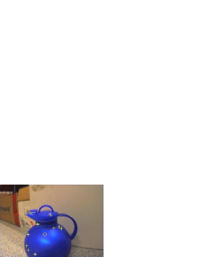
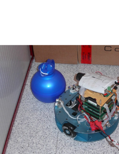
Figure 1: Learned Control Policy. Each row shows a different situation in the environment along with its corresponding learned policy. In the top row the robot is positioned directly in front of the target object. The crosses in the camera image mark detected pixels of the target color, and the circle indicates the assumed direction towards the target. The policy for this situation is shown in terms of the visual coordinates, i.e. only the $x$-$y$ camera view coordinates of the high dimensional policy are shown. Each point in the policy graph indicates, with an arrow, the direction the robot should move if the circle, shown in the image is at that point in the visual field (left arrow means move left, right=right, up=forward, down=backwards, and no arrow=stand still. For instance, in this case, the robot should move forward because the circle lies in a part of the policy with an up arrow. In the bottom row the robot is almost touching the target. Here the policy is shown in terms of the subspace spanned by the two ultrasound distance sensors found at the fore and aft of the robot. The $b$-axis is the distance from the robot to the nearest obstacle in front, the $f$-axis behind. When the robot is with its back to an obstacle, and the way forward is clear (upper left corner of policy graph), it tends to go forward. When the way forward is obstructed, but there is nothing behind the robot (lower right corner), the robot tends to turn or move backward.

PC-NSM parameters. PC-NSM uses an $\epsilon$-greedy policy (Algorithm 1, line 13), with $\epsilon$ set to 0.3. This means that 30% of the time the robot selects an exploratory action. The appropriate number of nearest neighbors, $k$, used to select actions, depends upon the noisiness of the environment. The lower the noise, the smaller the $k$ that can be chosen. For the amount of noise in our sensors, we found that learning was fastest for $k=3$.

A common practice in toy reinforcement learning tasks such as discrete mazes is to use minimal reinforcement so that the agent is rewarded only when it reaches the goal. While such a formulation is useful to test algorithms in simulation, for real robots, this sparse, delayed reward forestalls learning as the agent can wander for long periods of time without reward, until finally happening upon the goal by accident.

Often there is specific domain knowledge that can incorporated into the reward function to provide intermediate reward that facilitates learning in robotic domains where exploration is costly [11]. The reward function we use is the sum of two components, one is obstacle-related, $R_{\mbox{\footnotesize obstacle}}$, and the other is target-related ,$R_{\mbox{\footnotesize target}}$:

$$R\;=\;\underbrace{-20/\max(0.01,\min(f,b))}_{R_{\mbox{\tiny obstacle}}}+\underbrace{p\cdot(500-50|x|-250y+c_{p})}_{R_{\mbox{\tiny target}}}$$ (5)

$R_{\mbox{\footnotesize target}}$ is largest when the robot is near to the goal and is looking directly towards it, smaller when the target is visible in the middle of the field of view, even smaller when the target is visible, but not in the center, and reaches its minimum when the target is not visible at all. $R_{\mbox{\footnotesize obstacle}}$ is negative when the robot is too close to some obstacle, except when the obstacle is the target itself, visible by the robot. It is important to note that the coefficients in equation 5 are specific to the robot and not the environment. They represent a one-time calibration of PC-NSM to the robot hardware being used.

Results. After taking between 1500 and 3000 actions the robot learns to avoid walls, reduce speed when approaching walls, look around for the goal, and go to the goal whenever it sees it. This is much faster compared to neural network based learners, e.g. [5], where 4000 episodes were required (resulting in more than 100’000 actions) to solve a simpler task in which the target was always within the perceptual field of the robot. Neither do we need a virtual model environment and manual quantization of the state space like in [14]. To our knowledge, our results are the fastest in terms of learning speed and use least quantization effort compared to all other methods to date, though we were unable to compare results directly on the hardware used by these competing approaches.

In the beginning of learning, corners pose serious difficulty causing the robot to get stuck and receive negative reinforcement for being too close to a wall. When the robot accidentally turns towards the target, it will quickly lose track of it. As learning progresses, the robot is able to recover (usually within one action) when an exploratory action causes it to turn away and loose sight of the target. The discounted metric allows the robot to use its history of real-valued observation states to remember that it had just seen the target in the recent past. Figure 1 shows the learned policy for this task.

Since the robot state space is perception-based (not $x$-$y$ coordinates on the floor as is the case in RL textbook examples), changing the position of the obstacles or target does not impede robot performance. Figure 2 shows learning in terms of immediate and average reward for a typical sequence of trials lasting a total of approximately 70 minutes. The dashed vertical lines in the two graphs indicate the beginning of a new trial. As learning progresses the robot is able to generalize from past experience and more quickly find the goal. After the first two trials, the robot starts to accumulate reward more rapidly in the third, after which the fourth trial is completed with very little deliberation. Figure 3 illustrates two such successful trials.

(a)                                                   (b)

Figure 2: PC-NSM learning performance. (a) The plot shows the reward the robot receives at each time-step during learning. (b) The plot shows the reward at each time-step averaged over all previous time-steps within the same trial. The dashed lines indicate the beginning of a new trial where the target is moved to a new location.

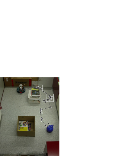
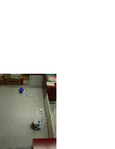
(a)                                                   (b)

Figure 3: Robot arena with learned trajectories. The picture shows two typical learning scenarios with the robot, obstacle, and target (blue plastic teapot) in their initial locations. The robot must learn to find the target using the limited visual field of its video camera, and move to it while avoiding obstacles. (a) The robot starts the trial facing away from the target before turning to its right, and navigating around the obstacle to the goal. Along the way it encounters two difficulties (shown by the rectangular highlights) caused first by going through the narrow passage and then by gap in the right wall where the front sonar returns a strong signal compared to the immediately surrounding wall because it is being specularly reflected. (b) The robot in an unoccluded arena after learning in trial (a). Here the robot drives almost directly to the target after turning to see it, but, again, is held up by the dark wall gap momentarily.

4 Discussion

We have developed a instance-based algorithm for mobile robot learning and successfully implemented it on an actual vision-controlled robot. The use of a metric state space allows our algorithm to work under weaker requirements and be more data-efficient compared to previous work in continuous reinforcement learning [3, 17, 19]. Using a metric instead of a discrete grid is a considerable relaxation of the programmer’s task, since it obviates the need to guess the correct scale for all the regions of the state space in advance. The algorithm explores the environment and learns directly on a mobile robot without using a hand-made computer model as an intermediate step, works in piecewise continuous perceptual spaces, and copes with partial observability.

The metric used in this paper worked well in our experiments, but a more powerful approach would be to allow the algorithm to select the appropriate metric for a given environment and task automatically. To choose between metrics, a criterion should be defined that determines which of a set of a priori equiprobable metrics $\{\mu_{1},\dots,\mu_{n}\}$ fits the given history of experimentation better. A useful criterion could be, for example, a generalization of the criteria used in the McCallum’s U-Tree algorithm [13] to decide whether a state should be split.

The current algorithm uses discrete actions so that there is a convenient way to group observation states. If the action space were continuous, the algorithm lacks a natural way to generalize between actions. A metric on the action space $\mu_{a}$ could be used within the observation-based neighborhood delimited by the current metric $\mu$. The agent could then randomly sample possible actions at the query point $h_{T}$ and obtain Q-values for each sampled action by computing the $\mu_{a}$-nearest neighbors within the $\mu$-neighborhood. Future work will explore this avenue.

Acknowledgments. This work is partially supported by CSEM Robotics Alpnach.

References

- [1] C. Anderson. Q-learning with hidden-unit restarting. In S. J. Hanson, J. D. Cowan, and C. L. Giles, editors, Advances in Neural Information Processing Systems 5, pages 81–88, San Mateo, CA, 1993. Morgan Kaufmann.
- [2] R. I. Brafman and M. Tennenholtz. R-max - a general polynomial time algorithm for near-optimal reinforcement learning. J. Mach. Learn. Res., 3:213–231, 2003.
- [3] K. Doya. Reinforcement learning in continuous time and space. Neural Computation, 12(1):219–245, 2000.
- [4] J. Forbes and D. Andre. Practical reinforcement learning in continuous domains. Technical Report UCB/CSD-00-1109, University of California, Berkeley, 2000.
- [5] M. Iida, M. Sugisaka, and K. Shibata. Application of direct-vision-based reinforcement learning to a real mobile robot with a CCD camera. In Proc. of AROB (Int’l Symp. on Artificial Life and Robotics) 8th, pages 86–89, 2003.
- [6] S. Kakade, M. Kearns, and J. Langford. Exploration in metric state spaces. In Machine Learning, Proceedings of the Twentieth International Conference (ICML 2003), August 21-24, 2003, Washington, DC, USA. AAAI Press, 2003.
- [7] M. Kearns and S. Singh. Near-optimal reinforcement learning in polynomial time. In Proc. 15th International Conf. on Machine Learning, pages 260–268. Morgan Kaufmann, San Francisco, CA, 1998.
- [8] M. J. Kearns and S. P. Singh. Near-optimal reinforcement learning in polynomial time. Machine Learning, 49(2-3):209–232, 2002.
- [9] L.-J. Lin. Self-improving reactive agents based on reinforcement learning, planning, and teaching. Machine Learning, 8(3):293–321, 1992.
- [10] L.-J. Lin and T. M. Mitchell. Memory approaches to reinforcement learning in non-Markovian domains. Technical Report CMU-CS-92-138, Carnegie Mellon University, School of Computer Science, May 1992.
- [11] M. J. Mataric. Reward functions for accelerated learning. In Machine Learning: Proceedings of the 11th Annual Conference, pages 181–189, 1994.
- [12] R. A. McCallum. Instance-based state identification for reinforcement learning. In G. Tesauro, D. Touretzky, and T. Leen, editors, Advances in Neural Information Processing Systems, volume 7, pages 377–384. The MIT Press, 1995.
- [13] R. A. McCallum. Learning to use selective attention and short-term memory in sequential tasks. In P. Maes, M. Mataric, J.-A. Meyer, J. Pollack, and S. W. Wilson, editors, From Animals to Animats 4: Proceedings of the Fourth International Conference on Simulation of Adaptive Behavior, Cambridge, MA, pages 315–324. MIT Press, Bradford Books, 1996.
- [14] T. Minato and M. Asada. Environmental change adaptation for mobile robot navigation. Journal of the Robotics Society of Japan, 18(5):706–712, 2000.
- [15] A. W. Moore. The parti-game algorithm for variable resolution reinforcement learning in multidimensional state-spaces. In J. D. Cowan, G. Tesauro, and J. Alspector, editors, Advances in Neural Information Processing Systems, volume 6, pages 711–718. Morgan Kaufmann Publishers, Inc., 1994.
- [16] S. Pareigis. Adaptive choice of grid and time in reinforcement learning. In NIPS ’97: Proceedings of the 1997 conference on Advances in neural information processing systems 10, pages 1036–1042, Cambridge, MA, USA, 1998. MIT Press.
- [17] J. C. Santamaria, R. S. Sutton, and A. Ram. Experiments with reinforcement learning in problems with continuous state and action spaces. Adapt. Behav., 6(2):163–217, 1997.
- [18] R. Schoknecht and M. Riedmiller. Learning to control at multiple time scales. In O. Kaynak, E. Alpaydin, E. Oja, and L. Xu, editors, Artificial Neural Networks and Neural Information Processing - ICANN/ICONIP 2003, Joint International Conference ICANN/ICONIP 2003, Istanbul, Turkey, June 26-29, 2003, Proceedings, volume 2714 of Lecture Notes in Computer Science. Springer, 2003.
- [19] W. D. Smart and L. P. Kaelbling. Practical reinforcement learning in continuous spaces. In Proc. 17th International Conf. on Machine Learning, pages 903–910. Morgan Kaufmann, San Francisco, CA, 2000.
- [20] R. Sutton and A. Barto. Reinforcement learning: An introduction. Cambridge, MA, MIT Press, 1998.
- [21] R. S. Sutton. First results with DYNA, an integrated architecture for learning, planning and reacting. In Proceedings of the AAAI Spring Symposium on Planning in Uncertain, Unpredictable, or Changing Environments, 1990.
- [22] R. S. Sutton. Generalization in reinforcement learning: Successful examples using sparse coarse coding. In D. S. Touretzky, M. C. Mozer, and M. E. Hasselmo, editors, Advances in Neural Information Processing Systems 8, pages 1038–1044. Cambridge, MA: MIT Press, 1996.