Abstract

Consider the problem of joint parameter estimation and prediction in a Markov random field: i.e., the model parameters are estimated on the basis of an initial set of data, and then the fitted model is used to perform prediction (e.g., smoothing, denoising, interpolation) on a new noisy observation. Working under the restriction of limited computation, we analyze a joint method in which the same convex variational relaxation is used to construct an M-estimator for fitting parameters, and to perform approximate marginalization for the prediction step. The key result of this paper is that in the computation-limited setting, using an inconsistent parameter estimator (i.e., an estimator that returns the “wrong” model even in the infinite data limit) can be provably beneficial, since the resulting errors can partially compensate for errors made by using an approximate prediction technique. En route to this result, we analyze the asymptotic properties of M-estimators based on convex variational relaxations, and establish a Lipschitz stability property that holds for a broad class of variational methods. We show that joint estimation/prediction based on the reweighted sum-product algorithm substantially outperforms a commonly used heuristic based on ordinary sum-product.

Keywords: Graphical model; Markov random field; belief propagation; sum-product algorithm; variational method; parameter estimation; pseudolikelihood; prediction error; Lipschitz stability; mixture of Gaussian.

1 Introduction

Graphical models such as Markov random fields (MRFs) are widely used in many application domains, including spatial statistics, statistical signal processing, and communication theory. A fundamental limitation to their practical use is the infeasibility of computing various statistical quantities (e.g., marginals, data likelihoods etc.); such quantities are of interest both Bayesian and frequentist settings. Sampling-based methods, especially those of the Markov chain Monte Carlo (MCMC) variety [14, 18], represent one approach to obtaining stochastic approximations to marginals and likelihoods. A disadvantage of sampling methods is their relatively high computational cost. For instance, in applications with severe limits on delay and computational overhead (e.g., error-control coding, real-time tracking, video compression), MCMC methods are likely to be overly slow. It is thus of considerable interest for various application domains to consider less computationally intensive methods for generating approximations to marginals, log likelihoods, and other relevant statistical quantities.

Variational methods are one class of techniques that can be used to generate deterministic approximations in Markov random fields (MRFs). At the foundation of these methods is the fact that for a broad class of MRFs, the computation of the log likelihood and marginal probabilities can be reformulated as a convex optimization problem (see [32, 30] for an overview). Although this optimization problem is intractable to solve exactly for general MRFs, it suggests a principled route to obtaining approximations—namely, by relaxing the original optimization problem, and taking the optimal solutions to the relaxed problem as approximations to the exact values. In many cases, optimization of the relaxed problem can be carried out by “message-passing” algorithms, in which neighboring nodes in the Markov random field convey statistical information (e.g., likelihoods) by passing functions or vectors (referred to as messages).

Estimating the parameters of a Markov random field from data poses another significant challenge. A direct approach—for instance, via (regularized) maximum likelihood estimation—entails evaluating the cumulant generating (or log partition) function, which is computationally intractable for general Markov random fields. One viable option is the pseudolikelihood method [3, 4], which can be shown to produce consistent parameter estimates under suitable assumptions, though with an associated loss of statistical efficiency. Other researchers have studied algorithms for ML estimation based on stochastic approximation [36, 1], which again are consistent under appropriate assumptions, but can be slow to converge.

1.1 Overview

As illustrated in Figure 1, the problem domain of interest in this paper is that of joint estimation and prediction in a Markov random field. More precisely, given samples $\{X^{1},\ldots,X^{n}\}$ from some unknown underlying model $p(\,\cdot\,;{\theta^{*}})$, the first step is to form an estimate of the model parameters. Now suppose that we are given a noisy observation of a new sample path $Z\sim p(\,\cdot\,;{\theta^{*}})$, and that we wish to form a (near)-optimal estimate of $Z$ using the fitted model, and the noisy observation (denoted $Y$). Examples of such prediction problems include signal denoising, image interpolation, and decoding of error-control codes. Disregarding any issues of computational cost and speed, one could proceed via Route A in Figure 1—that is, one could envisage first using a standard technique (e.g., regularized maximum likelihood) for parameter estimation, and then carrying out the prediction step (which might, for instance, involve computing certain marginal probabilities) by Monte Carlo methods.

This paper, in contrast, is concerned with the computation-limited setting, in which both sampling or brute force methods are overly intensive. With this motivation, a number of researchers have studied the use of approximate message-passing techniques, both for problems of prediction [10, 11, 15, 23, 27, 34, 35] as well as for parameter estimation [13, 22, 25, 28]. However, despite their wide-spread use, the theoretical understanding of such message-passing techniques remains limited, especially for parameter estimation. Consequently, it is of considerable interest to characterize and quantify the loss in performance incurred by using computationally tractable methods versus exact methods (i.e., Route B versus A in Figure 1). More specifically, our analysis applies to variational methods that are based convex relaxations. This class includes a broad range of extant methods—among them the tree-reweighted sum-product algorithm [29], reweighted forms of generalized belief propagation [34], and semidefinite relaxations [32]. Moreover, it is straightforward to modify other message-passing methods (e.g., expectation propagation [15]) so as to “convexify” them.

At a high level, the key idea of this paper is the following: given that approximate methods can lead to errors at both the estimation and prediction phases, it is natural to speculate that these sources of error might be arranged to partially cancel one another. The theoretical analysis of this paper confirms this intuition: we show that with respect to end-to-end performance, it is in fact beneficial, even in the infinite data limit, to learn the “wrong” the model by using inconsistent methods for parameter estimation. En route to this result, we analyze the asymptotic properties of M-estimators based on convex variational relaxations, and establish a Lipschitz stability property that holds for a broad class of variational methods. We show that joint estimation/prediction based on the reweighted sum-product algorithm substantially outperforms a commonly used heuristic based on ordinary sum-product.

\psfrag{#ydat#}{{\footnotesize$\{X^{i}\}$}}\psfrag{#compatapp#}{$\widehat{\theta}$}\psfrag{#compatml#}{${\theta^{*}}$}\psfrag{#xhatml#}{{\footnotesize{$\widehat{z}^{\operatorname{opt}}(Y;{\theta^{*}})$}}}\psfrag{#xhatapp#}{{\footnotesize{$\widehat{z}^{\operatorname{app}}(Y;\widehat{\theta})$}}}\psfrag{#xnew#}{{\footnotesize{$Y$}}}\psfrag{#err#}{{\footnotesize{$\operatorname{Error:}\;\;\|\widehat{z}^{\operatorname{opt}}(Y;{\theta^{*}})-\widehat{z}^{\operatorname{app}}(Y;\widehat{\theta})\|$}}}\includegraphics[keepaspectratio,width=446.2658pt]{good_estpluspred_block.eps}

Figure 1: Route A: computationally intractable combination of parameter estimation and prediction. Route B: computationally efficient combination of approximate parameter estimation and prediction.

The remainder of this paper is organized as follows. Section 2 provides background on Markov random fields and associated variational representations, as well as the problem statement. In Section 3, we introduce the notion of a convex surrogate to the cumulant generating function, and then illustrate this notion via the tree-reweighted Bethe approximation [29]. In Section 4, we describe how any convex surrogate defines a particular joint scheme for parameter estimation and prediction. Section 5 provides results on the asymptotic behavior of the estimation step, as well as the stability of the prediction step. Section 6 is devoted to the derivation of performance bounds for joint estimation and prediction methods, with particular emphasis on the mixture-of-Gaussians observation model. In Section 7, we provide experimental results on the performance of a joint estimation/prediction method based on the tree-reweighted Bethe surrogate, and compare it to a heuristic method based on the ordinary belief propagation algorithm. We conclude in Section 8 with a summary and discussion of directions for future work.

2 Background and problem statement

2.1 Multinomial Markov random fields

Consider an undirected graph $G=(V,E)$, consisting of a set of vertices $V=\{1,\ldots,N\}$ and an edge set $E$. We associate to each vertex $s\in V$ a multinomial random variable $X_{s}$ taking values in the set ${\mathcal{X}}_{s}=\{0,1,\ldots,m-1\}$. We use the lower case letter $x_{s}$ to denote particular realizations of the random variable $X_{s}$ in the set ${\mathcal{X}}_{s}$. This paper makes use of the following exponential representation of a pairwise Markov random field over the multinomial random vector $X:=\{X_{s},\;s\in V\}$. We begin by defining, for each $j=1,\ldots,m-1$, the $\{0,1\}$-valued indicator function

$$\mathbb{I\,}_{j}[x_{s}] := \begin{cases}1&\mbox{if $x_{s}=j$}\\ 0&\mbox{otherwise}\end{cases}$$ (1)

These indicator functions can be used to define a potential function $\theta_{s}(\cdot):{\mathcal{X}}_{s}\rightarrow{\mathbb{R}}$ via

$$\theta_{s}(x_{s}) := \sum_{j=1}^{m-1}\theta_{s;j}\mathbb{I\,}_{j}[x_{s}]$$ (2)

where $\theta_{s}=\{\theta_{s;j},j=1,\ldots,m-1\}$ is the vector of exponential parameters associated with the potential. Our exclusion of the index $j=0$ is deliberate, so as to ensure that the collection of indicator functions $\phi_{s}(x_{s}):=\{\mathbb{I\,}_{j}[x_{s}],\;j=1,\ldots,m-1\}$ remain affinely independent. In a similar fashion, we define for any pair $(s,t)\in E$ the pairwise potential function

$$\theta_{st}(x_{s},x_{t}) := \sum_{j=1}^{m-1}\sum_{k=1}^{m-1}\theta_{st;jk}\mathbb{I\,}_{j}[x_{s}]\;\mathbb{I\,}_{k}[x_{t}],$$ (3)

where we use $\theta_{st}:=\{\theta_{st;jk},\;j,k=1,2,\ldots,m-1\}$ to denote the associated collection of exponential parameters, and $\phi_{st}(x_{s},x_{t}):=\{\mathbb{I\,}_{j}[x_{s}]\,\mathbb{I\,}_{k}[x_{s}],\;j,k=1,2,\ldots,m-1\}$ for the associated set of sufficient statistics.

Overall, the probability mass function of the multinomial Markov random field in exponential form can be written as

$$p(x\,;\,\theta) = \exp\big{\{}\sum_{s\in V}\theta_{s}(x_{s})+\sum_{(s,t)\in E}\theta_{st}(x_{s},x_{t})-A(\theta)\big{\}}.$$ (4)

Here the function

$$A(\theta) := \log\Big{[}\sum_{x\in{\mathcal{X}}^{N}}\exp\big{\{}\sum_{s\in V}\theta_{s}(x_{s})+\sum_{(s,t)\in E}\theta_{st}(x_{s},x_{t})\big{\}}\Big{]}$$ (5)

is the logarithm of the normalizing constant associated with $p(\cdot\,;\,\theta)$.

The collection of distributions thus defined can be viewed as a regular and minimal exponential family [5]. In particular, the exponential parameter $\theta$ and the vector of sufficient statistics $\phi$ are formed by concatenating the exponential parameters (respectively indicator functions) associated with each vertex and edge—viz.

$$\theta = \{\theta_{s},s\in V\}\cup\{\theta_{st},\;(s,t)\in E\}$$ (6a)

$$\phi(x) = \{\phi_{s}(x_{s}),s\in V\}\cup\{\phi_{st}(x_{s},x_{t}),\;(s,t)\in E\}$$ (6b)

This notation allows us to write equation (4) more compactly as $p(x\,;\,\theta)=\exp\{\langle\theta,\,\phi(x)\rangle-A(\theta)\}$. A quick calculation shows that $\theta\in{\mathbb{R}}^{d}$, where $d=N(m-1)+|E|\,(m-1)^{2}$ is the dimension of this exponential family.

The following properties of $A$ are well-known:

Lemma 1.

(a) The function $A$ is convex, and strictly so when the sufficient statistics are affinely independent.
(b) It is an infinitely differentiable function, with derivatives corresponding to cumulants. In particular, for any indices $\alpha,\beta\in\{1,\ldots,d\}$, we have

$$\frac{\partial{A}}{\partial{\theta_{\alpha}}}={\mathbb{E}}_{\theta}[\phi_{\alpha}(X)],\qquad\frac{\partial^{2}{A}}{\partial{\theta_{\alpha}}\,\partial{\theta_{\beta}}}=\operatorname{cov}_{\theta}\{\phi_{\alpha}(X),\,\phi_{\beta}(X)\},$$ (7)

where ${\mathbb{E}}_{\theta}$ and $\operatorname{cov}_{\theta}$ denote the expectation and covariance respectively.

We use $\mu\in{\mathbb{R}}^{d}$ to denote the vector of mean parameters defined element-wise by $\mu_{\alpha}={\mathbb{E}}_{\theta}[\phi_{\alpha}(X)]$ for any $\alpha\in\{1,\ldots,d\}$. A convenient property of the sufficient statistics $\phi$ defined in equations (1) and (2) is that these mean parameters correspond to marginal probabilities. For instance, when $\alpha=(s;j)$ or $\alpha=(st;jk)$, we have respectively

$$\mu_{s;j} = {\mathbb{E}}_{\theta}[\mathbb{I\,}_{j}[x_{s}]]=p(X_{s}=j\,;\,\theta),\quad\mbox{and}$$ (8a)

$$\mu_{st;jk} = {\mathbb{E}}_{\theta}\big{\{}\mathbb{I\,}_{j}[x_{s}]\,\mathbb{I\,}_{k}[x_{t}]\big{\}}=p(X_{s}=j,X_{t}=k\,;\,\theta).$$ (8b)

3 Construction of convex surrogates

This section is devoted to a systematic procedure for constructing convex functions that represent approximations to the cumulant generating function. We begin with a quick development of an exact variational principle, one which is intractable to solve in general cases. (More details on this exact variational principle can be found in the papers [30, 32].) Nonetheless, this exact variational principle is useful, in that various natural relaxations of the optimization problem can be used to define convex surrogates to the cumulant generating function. After a high-level description of such constructions in general, we then illustrate it more concretely with the particular case of the “convexified” Bethe entropy [29].

3.1 Exact variational representation

Since $A$ is a convex and continuous function (see Lemma 1), the theory of convex duality [19] guarantees that it has a variational representation, given in terms of its conjugate dual function $A^{*}:{\mathbb{R}}^{d}\rightarrow{\mathbb{R}}\cup\{+\infty\}$, of the following form

$$A(\theta) = \sup_{\mu\in{\mathbb{R}}^{d}}\big{\{}\theta^{T}\mu-A^{*}(\mu)\big{\}}.$$ (9)

In order to make effective use of this variational representation, it remains determine the form of the dual function. A useful fact is that the exponential family (4) arises naturally as the solution of an entropy maximization problem. In particular, consider the set of linear constraints

$${\mathbb{E}}_{p}[\phi(X)]\,:=\;\sum_{x\in{\mathcal{X}}^{N}}p(x)\phi_{\alpha}(x) = \mu_{\alpha}\quad\mbox{for $\alpha=1,\ldots,d$},$$ (10)

where $\mu\in{\mathbb{R}}^{d}$ is a set of target mean parameters. Letting $\mathcal{P}$ denote the set of all probability distributions with support on ${\mathcal{X}}^{N}$, consider the constrained entropy maximization problem: maximize the entropy $H(p):=-\sum_{x\in{\mathcal{X}}^{N}}p(x)\log p(x)$ subject to the constraints (10).

A first question is when there any distributions $p$ that satisfy the constraints (10). Accordingly, we define the set

$$\operatorname{MARG}_{\phi}(G) := \big{\{}\mu\in{\mathbb{R}}^{d}\,\big{|}\,\mu={\mathbb{E}}_{p}[\phi(X)]\quad\mbox{for some $p\in\mathcal{P}$}\big{\}},$$ (11)

corresponding to the set of $\mu$ for which the constraint set (10) is non-empty. For any $\mu\notin\operatorname{MARG}_{\phi}(G)$, the optimal value of the constrained maximization problem is $-\infty$ (by definition, since the problem is infeasible). Otherwise, it can be shown that the optimum is attained at a unique distribution in the exponential family, which we denote by $p(\cdot\,;\,\theta(\mu))$. Overall, these facts allow us to specify the conjugate dual function as follows:

$$A^{*}(\mu) = \begin{cases}-H(p(\cdot\,;\,\theta(\mu)))&\mbox{if $\mu\in\operatorname{MARG}_{\phi}(G)$}\\ +\infty&\mbox{otherwise.}\end{cases}$$ (12)

See the technical report [30] for more details of this dual calculation. With this form of the dual function, we are guaranteed that the cumulant generating function $A$ has the following variational representation:

$$A(\theta) = \max_{\mu\in\operatorname{MARG}_{\phi}(G)}\big{\{}\theta^{T}\mu-A^{*}(\mu)\big{\}}.$$ (13)

However, in general, solving the variational problem (13) is intractable. This intractability should not be a surprise, since the cumulant generating function is intractable to compute for a general graphical model. The difficulty arises from two sources. First, the constraint set $\operatorname{MARG}_{\phi}(G)$ is extremely difficult to characterize exactly for a general graph with cycles. For the case of a multinomial Markov random field (4), it can be seen (using the Minkowski-Weyl theorem) that $\operatorname{MARG}_{\phi}(G)$ is a polytope, meaning that it can be characterized by a finite number of linear constraints. The question, of course, is how rapidly this number of constraints grows with the number of nodes $N$ in the graph. Unless certain fundamental conjectures in computational complexity turn out to be false, this growth must be non-polynomial (see Deza and Laurent [7] for an in-depth discussion of the binary case). Tree-structured graphs are a notable exception, for which the junction tree theory [12] guarantees that the growth is only linear in $N$.

Second, the dual function $A^{*}$ lacks a closed-form representation for a general graph. Note in particular that the representation (12) is not explicit, since it requires solving a constrained entropy maximization problem in order to compute the value $H(p(\cdot\,;\,\theta(\mu)))$. Again, important exceptions to this rule are tree-structured graphs. Here a special case of the junction tree theory guarantees that any Markov random field on a tree $T=(V,E(T))$ can be factorized in terms of its marginals as follows

$$p(x\,;\,\theta(\mu)) = \prod_{s\in V}\mu_{s}(x_{s})\prod_{(s,t)\in E(T)}\frac{\mu_{st}(x_{s},x_{t})}{\mu_{s}(x_{s})\mu_{t}(x_{t})}.$$ (14)

Consequently, in this case, the negative entropy (and hence the dual function) can be computed explicitly as

$$-A^{*}(\mu;T) = \sum_{s\in V}H_{s}(\mu_{s})-\sum_{(s,t)\in E(T)},I_{st}(\mu_{st})$$ (15)

where $H_{s}(\mu_{s})\;:=\;-\sum_{x_{s}}\mu_{s}(x_{s})\log\mu_{s}(x_{s})$ and $I_{st}(\mu_{st}):=\sum_{x_{s},x_{t}}\mu_{st}(x_{s},x_{t})\log\frac{\mu_{st}(x_{s},x_{t})}{\mu_{s}(x_{s})\mu_{t}(x_{t})}$ are the singleton entropy and mutual information, respectively, associated with the node $s\in V$ and edge $(s,t)\in E(T)$. For a general graph with cycles, in contrast, the dual function lacks such an explicit form, and is not easy to compute.

Given these challenges, it is natural to consider approximations to $A^{*}$ and $\operatorname{MARG}_{\phi}(G)$. As we discuss in the following section, the resulting relaxed optimization problem defines a convex surrogate to the cumulant generating function.

3.2 Convex surrogates to the cumulant generating function

We now describe a general procedure for constructing convex surrogates to the cumulant generating function, consisting of two main ingredients. Given the intractability of characterizing the marginal polytope $\operatorname{MARG}_{\phi}(G)$, it is natural to consider a relaxation. More specifically, let $\operatorname{REL}_{\phi}(G)$ be a convex and compact set that acts as an outer bound to $\operatorname{MARG}_{\phi}(G)$. We use $\tau$ to denote elements of $\operatorname{REL}_{\phi}(G)$, and refer to them as pseudomarginals since they represent relaxed versions of local marginals. The second ingredient is to designed to sidestep the intractability of the dual function: in particular, let $B^{*}$ be a strictly convex and twice continuously differentiable approximation to $A^{*}$. We require that the domain of $B^{*}$ (i.e., $\operatorname{dom}(B^{*}):=\{\tau\in{\mathbb{R}}^{d}\,|\,B^{*}(\tau)<+\infty\}$) be contained within the relaxed constraint set $\operatorname{REL}_{\phi}(G)$.

By combining these two approximations, we obtain a convex surrogate $B$ to the cumulant generating function, specified via the solution of the following relaxed optimization problem

$$B(\theta) := \max_{\tau\in\operatorname{REL}_{\phi}(G)}\big{\{}\theta^{T}\tau-B^{*}(\tau)\big{\}}.$$ (16)

Note the parallel between this definition (16) and the variational representation of $A$ in equation (13).

The function $B$ so defined has several desirable properties, as summarized in the following proposition:

Proposition 1.

Any convex surrogate $B$ defined via (16) has the following properties:

1. For each $\theta\in{\mathbb{R}}^{d}$, the optimum defining $B$ is attained at a unique point $\tau(\theta)$.

2. The function $B$ is convex on ${\mathbb{R}}^{d}$.

3. It is differentiable on ${\mathbb{R}}^{d}$, and more specifically:

   $$\nabla B(\theta) = \tau(\theta).$$ (17)

Proof.

(i) By construction, the constraint set $\operatorname{REL}_{\phi}(G)$ is compact and convex, and the function $B^{*}$ is strictly convex, so that the optimum is attained at a unique point $\tau(\theta)$.
(ii) Observe that $B$ is defined by the maximum of a collection of functions linear in $\theta$, which ensures that it is convex [2].
(iii) Finally, the function $\theta^{T}\tau-B^{*}(\tau)$ satisfies the hypotheses of Danskin’s theorem [2], from which we conclude that $B$ is differentiable with $\nabla B(\theta)=\tau(\theta)$ as claimed. ∎

Given the interpretation of $\tau(\theta)$ as a pseudomarginal, this last property of $B$ is analogous to the well-known cumulant generating property of $A$—namely, $\nabla A(\theta)=\mu(\theta)$—as specified in Lemma 1.

3.3 Convexified Bethe surrogate

The following example provides a more concrete illustration of this constructive procedure, using a tree-based approximation to the marginal polytope, and a convexifed Bethe entropy approximation [29]. As with the ordinary Bethe approximation [35], the cost function and constraint set underlying this approximation are exact for any tree-structured Markov random field.

Relaxed polytope:

We begin by describing a relaxed version $\operatorname{REL}_{\phi}(G)$ of the marginal polytope $\operatorname{MARG}_{\phi}({\boldsymbol{\phi}})$. Let $\tau_{s}$ and $\tau_{st}$ represent a collection of singleton and pairwise pseudomarginals, respectively, associated with vertices and edges of a graph $G$. These quantities, as locally valid marginal distributions, must satisfy the following set of local consistency conditions:

$$\operatorname{LOCAL}_{\phi}(G) := \big{\{}\tau\in{\mathbb{R}}^{d}_{+}\,\big{|}\,\sum_{x_{s}}\tau_{s}(x_{s})=1,\;\;\sum_{x_{t}}\tau_{st}(x_{s},x_{t})=\tau_{s}(x_{s})\big{\}}.$$ (18)

By construction, we are guaranteed the inclusion $\operatorname{MARG}_{\phi}(G)\subset\operatorname{LOCAL}_{\phi}(G)$. Moreover, a special case of the junction tree theory [12] guarantees that equality holds when the underlying graph is a tree (in particular, any $\tau\in\operatorname{LOCAL}_{\phi}(G)$ can be realized as the marginals of the tree-structured distribution of the form (14)). However, the inclusion is strict for any graph with cycles; see Appendix A for further discussion of this issue.

Entropy approximation:

We now define an entropy approximation $B^{*}_{\rho}$ that is finite for any pseudomarginal $\tau$ in the relaxed set $\operatorname{LOCAL}_{\phi}(G)$. We begin by considering a collection $\{T\in\mathfrak{T}\}$ of spanning trees associated with the original graph. Given $\tau\in\operatorname{LOCAL}_{\phi}(G)$, there is—for each spanning tree $T$—a unique tree-structured distribution that has marginals $\tau_{s}$ and $\tau_{st}$ on the vertex set $V$ and edge set $E(T)$ of the tree. Using equations (14) and (15), the entropy of this tree-structured distribution can be computed explicitly. The convexified Bethe entropy approximation is based on taking a convex combination of these tree entropies, where each tree is weighted by a probability $\rho(T)\in[0,1]$. Doing so and expanding the sum yields

$$B^{*}_{\rho}(\tau) := \sum_{T\in\mathfrak{T}}\rho(T)\Big{\{}\sum_{s\in V}H_{s}(\tau_{s})-\sum_{(s,t)\in E(T)}I_{st}(\tau_{st})\Big{\}}\;=\;\sum_{s\in V}H_{s}(\tau_{s})-\sum_{(s,t)\in E}\rho_{st}I_{st}(\tau_{st}),$$ (19)

where $\rho_{st}=\sum_{T}\rho(T)\mathbb{I\,}[(s,t)\in T]$ are the edge appearance probabilities defined by the distribution $\rho$ over the tree collection. By construction, the function $B^{*}_{\rho}$ is differentiable; moreover, it can be shown [29] that it is strictly convex for any vector $\{\rho_{st}\}$ of strictly positive edge appearance probabilities.

Bethe surrogate and reweighted sum-product:

We use these two ingredients—the relaxation $\operatorname{LOCAL}_{\phi}(G)$ of the marginal polytope, and the convexified Bethe entropy approximation (19)—to define the following convex surrogate

$$B_{\rho}(\theta) := \max_{\tau\in\operatorname{LOCAL}_{\phi}(G)}\big{\{}\theta^{T}\tau-B^{*}_{\rho}(\tau)\big{\}}.$$ (20)

Since the conditions of Proposition 1 are satisfied, we are guaranteed that $B_{\rho}$ is convex and differentiable on ${\mathbb{R}}^{d}$, and moreover that $\nabla B_{\rho}(\theta)=\tau(\theta)$, where (for each $\theta\in{\mathbb{R}}^{d}$) the quantity $\tau(\theta)$ denotes the unique optimum of problem (20). Perhaps most importantly, the optimizing pseudomarginals $\tau(\theta)$ can be computed efficiently using a tree-reweighted variant of the sum-product message-passing algorithm [29]. This method operates by passing “messages”, which in the multinomial case are simply $m$-vectors of non-negative numbers, along edges of the graph. We use $M_{ts}=\{M_{ts}(i),i=0,\ldots,m-1\}$ to represent the message passed from node $t$ to node $s$. In the tree-reweighted variant, these messages are updated according to the following recursion

$$M_{ts}(x_{s}) \leftarrow \sum_{x_{t}}\exp\Big{\{}\theta_{t}(x_{t})\frac{\theta_{st}(x_{s},x_{t})}{\rho_{st}}\Big{\}}\frac{\prod_{u\in\Gamma(t)\backslash s}\big{[}M_{ut}(x_{t})\big{]}^{\rho_{ut}}}{\big{[}M_{st}(x_{t})\big{]}^{1-\rho_{st}}}.$$ (21)

Upon convergence of the updates, the fixed point messages $M^{*}$ yield the unique global optimum of the optimization problem (20) via the following equations

$$\tau_{s}(x_{s};\theta) \propto \exp\big{\{}\theta_{s}(x_{s})\big{\}}\prod_{u\in\Gamma(s)}\big{[}M_{us}(x_{s})\big{]}^{\rho_{us}},\quad\mbox{and}$$ (22a)

$$\tau_{st}(x_{s},x_{t};\theta) \propto \exp\big{\{}\theta_{s}(x_{s})+\theta_{t}(x_{t})+\frac{\theta_{st}(x_{s},x_{t})}{\rho_{st}}\big{\}}\frac{\prod\limits_{u\in\Gamma(s)}\big{[}M_{us}(x_{s})\big{]}^{\rho_{us}}\;\prod\limits_{v\in\Gamma(s)}\big{[}M_{vs}(x_{s})\big{]}^{\rho_{vs}}}{M_{st}(x_{t})\;M_{ts}(x_{s})}$$ (22b)

Further details on these updates and their properties can be found in the paper [29].

4 Joint estimation and prediction using surrogates

We now turn to consideration of how convex surrogates, as constructed by the procedure described in the previous section, are useful for both approximate parameter estimation as well as prediction.

4.1 Approximate parameter estimation

Suppose that we are given i.i.d. samples $\{X^{1},\ldots,X^{n}\}$ from an MRF of the form (4), where the underlying true parameter ${\theta^{*}}$ is unknown. One standard way in which to estimate ${\theta^{*}}$ is via maximum likelihood (possibly with an additional regularization term); in this particular exponential family setting, it is straightforward to show that the (normalized) log likelihood takes the form

$$\ell(\theta) = \langle\widehat{\mu}^{n},\,\theta\rangle-A(\theta)-\lambda^{n}R(\theta)$$ (23)

where function $R$ is a regularization term with an associated (possibly data-dependent) weight $\lambda^{n}$. The quantities $\widehat{\mu}^{n}:=\frac{1}{n}\sum_{i=1}^{n}\phi(X^{i})$ are the empirical moments defined by the data. For the indicator-based exponential representation (8), these empirical moments correspond to a set of singleton and pairwise marginal distributions, denoted $\widehat{\mu}^{n}_{s}$ and $\widehat{\mu}^{n}_{st}$ respectively.

It is intractable to maximize the regularized likelihood directly, due to the presence of the cumulant generating function $A$. Thus, a natural thought is to use the convex surrogate $B$ to define an alternative estimator obtained by maximizing the regularized surrogate likelihood:

$$\ell_{B}(\theta) := \langle\widehat{\mu}^{n},\,\theta\rangle-B(\theta)-\lambda^{n}R(\theta).$$ (24)

By design, the surrogate $B$ and hence the surrogate likelihood $\ell_{B}$, as well as their derivatives, can be computed in a straightforward manner (typically by some sort of message-passing algorithm). It is thus straightforward to compute the parameter $\widehat{\theta}^{n}$ achieving the maximum of the regularized surrogate likelihood (for instance, gradient descent would a simple though naive method).

For the tree-reweighted Bethe surrogate (20), we have shown in previous work [28] that in the absence of regularization, the optimal parameter estimates $\widehat{\theta}^{n}$ have a very simple closed-form solution, specified in terms of the weights $\rho_{st}$ and the empirical marginals $\widehat{\mu}$. (We make use of this closed form in our experimental comparison in Section 7; see equation (47).) If a regularizing term is added, these estimates no longer have a closed-form solution, but the optimization problem (24) can still be solved efficiently using the tree-reweighted sum-product algorithm [28, 29].

4.2 Joint estimation and prediction

Using such an estimator, we now consider a joint approach to estimation and prediction. Recalling the basic set-up, we are given an initial set of i.i.d. samples $\{x^{1},\ldots,x^{n}\}$ from $p(\cdot\,;\,{\theta^{*}})$, where the true model parameter ${\theta^{*}}$ is unknown. These samples are used to form an estimate of the Markov random field. We are then given a noisy observation $y$ of a new sample $z\sim p(\cdot\,;\,{\theta^{*}})$, and the goal is to use this observation in conjunction with the fitted model to form a near-optimal estimate of $z$. The key point is that the same convex surrogate $B$ is used both in forming the surrogate likelihood (24) for approximate parameter estimation, and in the variational method (16) for performing prediction.

For a given fitted model parameter $\theta\in{\mathbb{R}}^{d}$, the central object in performing prediction is the posterior distribution $p(z\,\mid\,y\,;\,\theta)\propto p(z\,;\,\theta)\;p(y\,|\,z)$. In the exponential family setting, for a fixed noisy observation $y$, this posterior can always be written as a new exponential family member, described by parameter $\theta+\gamma(y)$. (Here the term $\gamma(y)$ serves to incorporate the effect of the noisy observation.) With this set-up, the procedure consists of the following steps:

Joint estimation and prediction: 1. Form an approximate parameter estimate $\widehat{\theta}^{n}$ from an initial set of i.i.d. data $\{x^{1},\ldots,x^{n}\}$ by maximizing the (regularized) surrogate likelihood $\ell_{B}$. 2. Given a new noisy observation $y$ (i.e., a contaminated version of $z\sim p(\cdot\,;\,{\theta^{*}})$) specified by a factorized conditional distribution of the form $p(y\,|\,z)=\prod_{s=1}^{N}p(y_{s}\,|\,z_{s})$, incorporate it into the model by forming the new exponential parameter $$\widehat{\theta}^{n}_{s}(\,\cdot\,)+\gamma_{s}(y)$$ (25) where $\gamma_{s}(y)$ merges the new data with the fitted model $\widehat{\theta}^{n}$. (The specific form of $\gamma$ depends on the observation model.) 3. Using the message-passing algorithm associated with the convex surrogate $B$, compute approximate marginals $\tau(\widehat{\theta}+\gamma)$ for the distribution that combines the fitted model with the new observation. Use these approximate marginals to construct a prediction $\widehat{z}(y;\tau)$ of $z$ based on the observation $y$ and pseudomarginals $\tau$.

Examples of the prediction task in the final step include smoothing (e.g., denoising of a noisy image) and interpolation (e.g., in the presence of missing data). We provide a concrete illustration of such a prediction problem in Section 6 using a mixture-of-Gaussians observation model. The most important property of this joint scheme is that the convex surrogate $B$ underlies both the parameter estimation phase (used to form the surrrogate likelihood), and the prediction phase (used in the variational method for computing approximate marginals). It is this matching property that will be shown to be beneficial in terms of overall performance.

5 Analysis

In this section, we turn to the analysis of the surrogate-based method for estimation and prediction. We begin by exploring the asymptotic behavior of the parameter estimator. We then prove a Lipschitz stability result applicable to any variational method that is based on a strongly concave entropy approximation. This stability result plays a central role in our subsequent development of bounds on the performance loss in Section 6.

5.1 Estimator asymptotics

We begin by considering the asymptotic behavior of the parameter estimator $\widehat{\theta}^{n}$ defined by the surrogate likelihood (24). Since this parameter estimator is a particular type of $M$-estimator, its asymptotic behavior can be investigated using standard methods, as summarized in the following:

Proposition 2.

Let $B$ be a strictly convex surrogate to the cumulant generating function, defined via equation (16) with a strictly concave entropy approximation $-B^{*}$. Consider the sequence of parameter estimates $\{\widehat{\theta}^{n}\}$ given by

$$\widehat{\theta}^{n} := \arg\max_{\theta\in{\mathbb{R}}^{d}}\left\{\langle\widehat{\mu}^{n},\,\theta\rangle-B(\theta)-\lambda^{n}R(\theta)\right\}$$ (26)

where $R$ is a non-negative and convex regularizer, and the regularization parameter satisfies $\lambda^{n}=o(\frac{1}{\sqrt{n}})$.

Then for a general graph with cycles, the following results hold:

1. we have $\widehat{\theta}^{n}\stackrel{{\scriptstyle p}}{{\longrightarrow}}\widehat{\theta}$, where $\widehat{\theta}$ is (in general) distinct from the true parameter ${\theta^{*}}$.

2. the estimator is asymptotically normal:

   $$\sqrt{n}\big{[}\widehat{\theta}^{n}-\widehat{\theta}\big{]} \stackrel{{\scriptstyle d}}{{\longrightarrow}} N\biggr{(}0,\,\big{(}\nabla^{2}B(\widehat{\theta})\big{)}^{-1}\nabla^{2}A({\theta^{*}})\big{(}\nabla^{2}B(\widehat{\theta})\big{)}^{-1}\biggr{)}$$

Proof.

By construction, the convex surrogate $B$ and the (negative) entropy approximation $B^{*}$ are a Fenchel-Legendre conjugate dual pair. From Proposition 1, the surrogate $B$ is differentiable. Moreover, the strict convexity of $B$ and $B^{*}$ ensure that the gradient mapping $\nabla B$ is one-to-one and onto the relative interior of the constraint set $\operatorname{REL}_{\phi}(G)$ (see Section 26 of Rockafellar [19]). Moreover, the inverse mapping $(\nabla B)^{-1}$ exists, and is given by the dual gradient $\nabla B^{*}$.

Let $\mu^{*}$ be the moment parameters associated with the true distribution ${\theta^{*}}$ (i.e., $\mu^{*}={\mathbb{E}}_{{\theta^{*}}}[\phi(X)]$). In the limit of infinite data, the asymptotic value of the parameter estimate is defined by

$$\nabla B(\widehat{\theta})=\mu^{*}.$$ (27)

Note that $\mu^{*}$ belongs to the relative interior of $\operatorname{MARG}_{\phi}(G)$, and hence to the relative interior of $\operatorname{REL}_{\phi}(G)$. Therefore, equation (27) has a unique solution $\widehat{\theta}=\nabla^{-1}B(\mu^{*})$.

By strict convexity, the regularized surrogate likelihood (26) has a unique global maximum. Let us consider the optimality conditions defining this unique maximum $\widehat{\theta}^{n}$; they are given by $\nabla B(\widehat{\theta}^{n})=\widehat{\mu}^{n}-\lambda^{n}\partial R(\widehat{\theta}^{n})$, where $\partial R(\widehat{\theta}^{n})$ denotes an arbitrary element of the subdifferential of the convex function $R$ at the point $\widehat{\theta}^{n}$. We can now write

$$\nabla B(\widehat{\theta}^{n})-\nabla B(\widehat{\theta}) = \left[\widehat{\mu}^{n}-\mu^{*}\right]-\lambda^{n}\partial R(\widehat{\theta}^{n}).$$ (28)

Taking inner products with the difference $\widehat{\theta}^{n}-\widehat{\theta}$ yields

$$0\;\stackrel{{\scriptstyle(a)}}{{\leq}}\;\left[B(\widehat{\theta}^{n})-\nabla B(\widehat{\theta})\right]^{T}\;\left[\widehat{\theta}^{n}-\widehat{\theta}\right]\;\leq\;\left[\widehat{\mu}^{n}-\mu^{*}\right]^{T}\left[\widehat{\theta}^{n}-\widehat{\theta}\right]+\lambda^{n}\partial R(\widehat{\theta}^{n})^{T}\left[\widehat{\theta}-\widehat{\theta}^{n}\right],$$ (29)

where inequality (a) follows from the convexity of $B$. From the convexity and non-negativity of $R$, we have

$$\lambda^{n}\partial R(\widehat{\theta}^{n})^{T}\left[\widehat{\theta}-\widehat{\theta}^{n}\right]\;\leq\;\lambda^{n}\left[R(\widehat{\theta})-R(\widehat{\theta}^{n})\right]\;\leq\;\lambda^{n}R(\widehat{\theta}).$$

Applying this inequality and Cauchy-Schwartz to equation (29) yields

$$0\;\leq\;\left[B(\widehat{\theta}^{n})-\nabla B(\widehat{\theta})\right]^{T}\;\left[\frac{\widehat{\theta}^{n}-\widehat{\theta}}{\|\widehat{\theta}^{n}-\widehat{\theta}\|}\right]\;\leq\;\|\widehat{\mu}^{n}-\mu^{*}\|+\lambda^{n}R(\widehat{\theta})$$ (30)

Since $\lambda^{n}=o(1)$ by assumption and $\|\widehat{\mu}^{n}-\mu^{*}\|=o_{p}(1)$ by the weak law of large numbers, the quantity $\left[B(\widehat{\theta}^{n})-\nabla B(\widehat{\theta})\right]^{T}\;\left[\frac{\widehat{\theta}^{n}-\widehat{\theta}}{\|\widehat{\theta}^{n}-\widehat{\theta}\|}\right]$ converges in probability to zero. By the strict convexity of $B$, this fact implies that $\widehat{\theta}^{n}$ converges in probability to $\widehat{\theta}$, thereby completing the proof of part (a).

To establish part (b), we observe that $\sqrt{n}\left[\widehat{\mu}^{n}-\mu^{*}\right]\stackrel{{\scriptstyle d}}{{\longrightarrow}}N(0,\nabla^{2}A({\theta^{*}}))$ by the central limit theorem. Using this fact and applying the delta method to equation (28) yields that

$$\sqrt{n}\nabla^{2}B(\widehat{\theta})\;\left[\widehat{\theta}^{n}-\widehat{\theta}\right]\stackrel{{\scriptstyle d}}{{\longrightarrow}}N\left(0,\nabla^{2}A({\theta^{*}})\right),$$

where we have used the fact that $\sqrt{n}\lambda^{n}=o(1)$. The strict convexity of $B$ guarantees that $\nabla^{2}B(\widehat{\theta})$ is invertible, so that claim (b) follows. ∎

A key property of the estimator is its inconsistency—i.e., the estimated model differs from the true model ${\theta^{*}}$ even in the limit of large data. Despite this inconsistency, we will see that the approximate parameter estimates $\widehat{\theta}^{n}$ are nonetheless useful for performing prediction.

5.2 Algorithmic stability

A desirable property of any algorithm—particularly one applied to statistical data—is that it exhibit an appropriate form of stability with respect to its inputs. Not all message-passing algorithms have such stability properties. For instance, the standard sum-product message-passing algorithm, although stable for relatively weakly coupled MRFs [11, 24], can be highly unstable in other regimes due to the appearance of multiple local optima in the non-convex Bethe problem. However, previous experimental work has shown that methods based on convex relaxations, including the reweighted sum-product (or belief propagation) algorithm [28], reweighted generalized BP [34], and log-determinant relaxations [32] appear to be very stable. For instance, Figure 2 provides a simple illustration of the instability of the ordinary sum-product algorithm, contrasted with the stability of the tree-reweighted updates. Wiegerinck [34] provides similar results for reweighted forms of the generalized belief propagation.

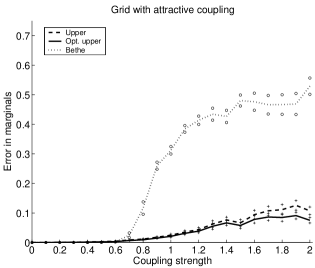
Figure 2: Contrast of the instability of the ordinary sum-product algorithm with the stability of the tree-reweighted version [29]. Results shown with a grid with $N=100$ nodes over a range of attractive coupling strengths. The ordinary sum-product undergoes a phase transition, after which the quality of marginal approximations degrades substantially. The tree-reweighted algorithm, shown for two different settings of the edge weights $\rho_{st}$, remains stable over the full range of coupling strengths. See Wainwright et al. [29] for full details.

Here we provide theoretical support for these empirical observations: in particular, we prove that, in sharp contrast to non-convex methods, any variational method based on a strongly convex entropy approximation is globally stable. This stability property plays a fundamental role in providing a performance guarantee on joint estimation/prediction methods.

We begin by noting that for a multinomial Markov random field (4), the computation of the exact marginal probabilities is a globally Lipschitz operation:

Lemma 2.

For any discrete Markov random field (4), there is a constant $L<+\infty$ such that

$$\|\mu(\theta+\delta)-\mu(\theta)\| \leq L\|\delta\|\qquad\quad\mbox{for all $\theta,\delta\in{\mathbb{R}}^{d}$.}$$ (31)

This lemma, which is proved in Appendix B, guarantees that small changes in the problem parameters—that is, “perturbations” $\delta$—lead to correspondingly small changes in the computed marginals.

Our goal is to establish analogous Lipschitz properties for variational methods. In particular, it turns out that any variational method based on a suitably concave entropy approximation satisfies such a stability condition. More precisely, a function $f:{\mathbb{R}}^{n}\rightarrow{\mathbb{R}}$ is strongly convex if there exists a constant $c>0$ such that $f(y)\geq f(x)+\nabla f(x)^{T}\,\big{(}y-x)+\frac{c}{2}\|y-x\|^{2}$ for all $x,y\in{\mathbb{R}}^{n}$. For a twice continuously differentiable function, this condition is equivalent to having the eigenspectrum of the Hessian $\nabla^{2}f(x)$ be uniformly bounded below by $c$. With this definition, we have:

Proposition 3.

Consider any strictly convex surrogate $B$ based on a strongly concave entropy approximation $-B^{*}$. Then there exists a constant $R<+\infty$ such that

$$\|\tau(\theta+\delta)-\tau(\theta)\| \leq R\|\delta\|\qquad\quad\mbox{for all $\theta,\delta\in{\mathbb{R}}^{d}$.}$$

Proof.

From Proposition 1, we have ${\tau}(\theta)=\nabla B(\theta)$, so that the statement is equivalent to the assertion that the gradient $\nabla B$ is a Lipschitz function. Applying the mean value theorem to $\nabla B$, we can write $\nabla B(\theta+\delta)-\nabla B(\theta)=\nabla^{2}B(\theta+t\delta)\delta$ where $t\in[0,1]$. Consequently, in order to establish the Lipschitz condition, it suffices to show that the spectral norm of $\nabla^{2}B(\gamma)$ is uniformly bounded above over all $\gamma\in{\mathbb{R}}^{d}$. Since $B$ and $B^{*}$ are a strictly convex Legendre pair, we have $\nabla^{2}B(\theta)=[\nabla^{2}B^{*}(\tau(\theta))]^{-1}$. By the strong convexity of $B^{*}$, we are guaranteed that the spectral norm of $\nabla^{2}B^{*}(\tau)$ is uniformly bounded away from zero, which yields the claim. ∎

Many existing entropy approximations can be shown to be strongly concave. In Appendix C, we provide a detailed proof of this fact for the convexified Bethe entropy (19).

Lemma 3.

For any set $\{\rho_{st}\}$ of strictly positive edge appearance probabilities, the convexified Bethe entropy (19) is strongly concave.

We note that the same argument can be used to establish strong concavity for the reweighted Kikuchi approximations studied by Wiegerinck [34]. Moreover, it can be shown that the Gaussian-based log-determinant relaxation considered in Wainwright and Jordan [31] is also strongly concave. For all of these variational methods, then, Proposition 3 guarantees that the pseudomarginal computation is globally Lipschitz stable, thereby providing theoretical confirmation of previous experimental results [34, 29, 31].

6 Performance bounds

In this section, we develop theoretical bounds on the performance loss of our approximate approach to joint estimation and prediction, relative to the unattainable Bayes optimum. So as not to unnecessarily complicate the result, we focus on the performance loss in the infinite data limit (i.e., for which the number of samples $n=+\infty$).

In the infinite data setting, the Bayes optimum is unattainable for two reasons:

1. it is based on knowledge of the exact parameter ${\theta^{*}}$, which is not easy to obtain.

2. it assumes (in the prediction phase) that computing exact marginal probabilities $\mu$ of the Markov random field is feasible.

Of these two difficulties, it is the latter assumption—regarding the computation of marginal probabilities—that is the most serious. As discussed earlier, there do exist computationally tractable estimators of ${\theta^{*}}$ that are consistent though not statistically efficient under appropriate conditions; one example is the pseudolikelihood method [3, 4] mentioned previously. On the other hand, MCMC methods may be used to generate stochastic approximations to marginal probabilities, but may require greater than polynomial complexity.

Recall from Proposition 2 that the parameter estimator based on the surrogate likelihood $\ell_{B}$ is inconsistent, in the sense that the parameter vector $\widehat{\theta}$ returned in the limit of infinite data is generally not equal to the true parameter ${\theta^{*}}$. Our analysis in this section will demonstrate that this inconsistency is beneficial.

6.1 Problem set-up

Although the ideas and techniques described here are more generally applicable, we focus here on a special observation model so as to obtain a concrete result.

Observation model:

In particular, we assume that the multinomial random vector $X=\{X_{s},\;s\in V\}$ defined by the Markov random field (4) is a label vector for the components in a finite mixture of Gaussians. For each node $s\in V$, we specify a new random variable $Z_{s}$ by the conditional distribution

$$p(Z_{s}=z_{s}\,|\,X_{s}=j)\sim N(\nu_{j},\sigma^{2}_{j})\quad\mbox{for $j\in\{0,1,\ldots,m-1\}$},$$

so that $Z_{s}$ is a mixture of $m$ Gaussians. Such Gaussian mixture models are widely used in spatial statistics as well as statistical signal and image processing [6, 17, 26].

Now suppose that we observe a noise-corrupted version of $z_{s}$— namely, a vector $Y$ of observations with components of the form

$$Y_{s}=\alpha Z_{s}+\sqrt{1-\alpha^{2}}W_{s},$$ (32)

where $W_{s}\sim N(0,1)$ is additive Gaussian noise, and the parameter $\alpha\in[0,1]$ specifies the signal-to-noise ratio (SNR) of the observation model. Note that $\alpha=0$ corresponds to pure noise, whereas $\alpha=1$ corresponds to completely uncorrupted observations.

Optimal prediction:

Our goal is to compute an optimal estimate $\widehat{z}(y)$ of $z$ as a function of the observation $Y=y$, using the mean-squared error as the risk function. The essential object in this computation is the posterior distribution $p(x\,\mid\,y\,;\,{\theta^{*}})=p(x\,;\,{\theta^{*}})\,p(y\,\mid\,x)$, where the conditional distribution $p(y\,\mid\,x)$ is defined by the observation model (32). As shown in the sequel, the posterior distribution (with $y$ fixed) can be expressed as an exponential family member of the form ${\theta^{*}}+\gamma(y)$ (see equation (39a)). Disregarding computational cost, it is straightforward to show that the optimal Bayes least squares estimator (BLSE) takes the form

$$\widehat{z}^{\operatorname{opt}}_{s}(Y;{\theta^{*}}) := \sum_{j=0}^{m-1}\mu_{s}(j;{\theta^{*}}+\gamma(Y))\biggr{[}\omega_{j}(\alpha)\big{(}Y_{s}-\nu_{j}\big{)}+\nu_{j}\biggr{]},$$ (33)

where $\mu_{s}(j;{\theta^{*}}+\gamma)$ denotes the marginal probability associated with the posterior distribution $p(x\,;\,{\theta^{*}}+\gamma)$, and

$$\omega_{j}(\alpha) := \frac{\alpha\sigma^{2}_{j}}{\alpha^{2}\sigma^{2}_{j}+(1-\alpha^{2})}$$ (34)

is the usual BLSE weighting for a Gaussian with variance $\sigma^{2}_{j}$.

Approximate prediction:

Since the marginal distributions $\mu_{s}(j;{\theta^{*}}+\gamma)$ are intractable to compute exactly, it is natural to consider an approximate predictor, based on a set $\tau$ of pseudomarginals computed from a variational relaxation. More explicitly, we run the variational algorithm on the parameter vector $\widehat{\theta}+\gamma$ that is obtained by combining the new observation $y$ with the fitted model $\widehat{\theta}$, and use the outputted pseudomarginals $\tau_{s}(\cdot;\widehat{\theta}+\gamma)$ as weights in the approximate predictor

$$\widehat{z}^{\operatorname{app}}_{s}(Y;\widehat{\theta}) := \sum_{j=0}^{m-1}\tau_{s}(j;\widehat{\theta}+\gamma(Y))\biggr{[}\omega_{j}(\alpha)\big{(}Y_{s}-\nu_{j}\big{)}+\nu_{j}\biggr{]},$$ (35)

where the weights $\omega$ are defined in equation (34).

We now turn to a comparison of the Bayes least-squares estimator (BLSE) defined in equation (33) to the surrogate-based predictor (35). Since (by definition) the BLSE is optimal for the mean-squared error (MSE), using the surrogate-based predictor will necessarily lead to a larger MSE. Our goal is to prove an upper bound on the maximal possible increase in this MSE, where the bound is specified in terms of the underlying model ${\theta^{*}}$ and the SNR parameter $\alpha$. More specifically, for a given problem, we define the mean-squared errors

$$\operatorname{R}^{\operatorname{app}}(\alpha,{\theta^{*}}):=\frac{1}{N}{\mathbb{E}}\|\widehat{z}^{\operatorname{opt}}(Y;{\theta^{*}})-Z\|^{2},\quad\mbox{and}\quad\operatorname{R}^{\operatorname{opt}}(\alpha,\widehat{\theta}):=\frac{1}{N}{\mathbb{E}}\|\widehat{z}^{\operatorname{app}}(Y;\widehat{\theta})-Z\|^{2},$$ (36)

of the Bayes-optimal and surrogate-based predictors, respectively. We seek upper bounds on the increase $\Delta\operatorname{R}(\alpha,{\theta^{*}},\widehat{\theta}):=\operatorname{R}^{\operatorname{app}}(\alpha,\widehat{\theta})-\operatorname{R}^{\operatorname{opt}}(\alpha,{\theta^{*}})$ of the approximate predictor relative to Bayes optimum.

6.2 Role of stability

Before providing a technical statement and proof, we begin with some intuition underlying the bounds, and the role of Lipschitz stability. First, consider the low SNR regime ($\alpha\approx 0$) in which the observation $Y$ is heavily corrupted by noise. In the limit $\alpha=0$, the new observations are pure noise, so that the prediction of $Z$ should be based simply on the estimated model—namely, the true model $p(\cdot\,;\,{\theta^{*}})$ in the Bayes optimal case, and the “incorrect” model $p(\cdot\,;\,\widehat{\theta})$ for the method based on surrogate likelihood. The key point here is the following: by properties of the MLE and surrogate-based estimator, the following equalities hold:

$$\nabla A({\theta^{*}})\;\stackrel{{\scriptstyle(a)}}{{=}}\;\mu({\theta^{*}})\;\stackrel{{\scriptstyle(b)}}{{=}}\;\mu^{*}\;\stackrel{{\scriptstyle(c)}}{{=}}\;\tau(\widehat{\theta})\;\stackrel{{\scriptstyle(d)}}{{=}}\;\nabla B(\widehat{\theta}).$$ (37)

Here equality (a) follows from Lemma 1, whereas equality (b) follows from the moment-matching property of the MLE in exponential families. Equalities (c) and (d) hold from the Proposition 1 and the pseudomoment-matching property of the surrogate-based parameter estimator (see proof of Proposition 2). As a key consequence, it follows that the combination of surrogate-based estimation and prediction is functionally indistinguishable from the Bayes-optimal behavior in the limit of $\alpha=0$. More specifically, in the limiting case, the errors systematically introduced by the inconsistent learning procedure are cancelled out exactly by the approximate variational method for computing marginal distributions. Of course, exactness for $\alpha=0$ is of limited interest; however, when combined with the Lipschitz stability ensured by Proposition 3, it allows us to gain good control of the low SNR regime. At the other extreme of high SNR ($\alpha\approx 1$), the observations are nearly perfect, and hence dominate the behavior of the optimal estimator. More precisely, for $\alpha$ close to $1$, we have $\omega_{j}(\alpha)\approx 1$ for all $j=0,1,\ldots,{m}-1$, so that $\widehat{z}^{\operatorname{opt}}(Y;{\theta^{*}})\approx Y\approx\widehat{z}^{\operatorname{app}}(Y;\widehat{\theta})$. Consequently, in the high SNR regime, accuracy of the marginal computation has little effect on the accuracy of the predictor.

6.3 Bound on performance loss

Although bounds of this nature can be developed in more generality, for simplicity in notation we focus here on the case of ${m}=2$ mixture components. We begin by introducing the factors that play a role in our bound on the performance loss $\Delta\operatorname{R}(\alpha,{\theta^{*}},\widehat{\theta})$. First, the Lipschitz stability enters in the form of the quantity:

$$L({\theta^{*}};\widehat{\theta}) := \sup_{\delta\in{\mathbb{R}}^{d}}\sigma_{\operatorname{max}}\big{(}\nabla^{2}A({\theta^{*}}+\delta)-\nabla^{2}B(\widehat{\theta}+\delta)\big{)},$$ (38)

where $\sigma_{\operatorname{max}}$ denotes the maximal singular value. Following the argument in the proof of Proposition 3, it can be seen that $L({\theta^{*}};\widehat{\theta})$ is finite.

Second, in order to apply the Lipschitz stability result, it is convenient to express the effect of introducing a new observation vector $y$, drawn from the additive noise observation model (32), as a perturbation of the exponential parameterization. In particular, for any parameter $\theta\in{\mathbb{R}}^{d}$ and observation $y$ from the model (32), the conditional distribution $p(x\,|\,y;\theta)$ can be expressed as $p(x;\theta+\gamma(y,\alpha))$, where the exponential parameter $\gamma(y,\alpha)$ has components

$$\gamma_{s} = \frac{1}{2}\Biggr{\{}\log\frac{\alpha^{2}\sigma_{0}^{2}+(1-\alpha^{2})}{\alpha^{2}\sigma^{2}_{1}+(1-\alpha^{2})}\;+\;\frac{(y_{s}-\alpha\nu_{0})^{2}}{\alpha^{2}\sigma^{2}_{0}+(1-\alpha^{2})}-\frac{(y_{s}-\alpha\nu_{1})^{2}}{\alpha^{2}\sigma^{2}_{1}+(1-\alpha^{2})}\Biggr{\}}\qquad\forall\;s\in V.$$ (39a)

$$\gamma_{st} = 0\qquad\qquad\qquad\qquad\forall\;(s,t)\in E.$$ (39b)

See Appendix D for a derivation of these relations.

Third, it is convenient to have short notation for the Gaussian estimators of each mixture component:

$$g_{j}(Y_{s};\alpha) := \omega_{j}(\alpha)\,\left(Y_{s}-\nu_{j}\right)+\nu_{j},\qquad\mbox{for $j=0,1$}$$ (40)

With this notation, we have the following

Theorem 1.

The MSE increase $\Delta\operatorname{R}(\alpha,{\theta^{*}},\widehat{\theta}):=\operatorname{R}(\alpha,\widehat{\theta})-\operatorname{R}(\alpha,{\theta^{*}})$ is upper bounded by

$$\Delta\operatorname{R}(\alpha,{\theta^{*}},\widehat{\theta}) \leq {\mathbb{E}}\left\{\min\left(1,\;L({\theta^{*}};\widehat{\theta})\frac{\|\gamma({{Y}};\alpha)\|_{2}}{\sqrt{N}}\right)\;\sqrt{\frac{\sum_{s=1}^{N}\left|g_{1}(Y_{s})-g_{0}(Y_{s})\right|^{4}}{N}}\right\}.$$ (41)

Before proving the bound (41), we begin by considering its behavior in a few special cases.

Effect of SNR:

First, consider the low SNR limit in which $\alpha\rightarrow 0^{+}$. In this limit, it can be seen that $\|\gamma({{Y}};\alpha)\|\rightarrow 0$, so that the the overall bound $\Delta\operatorname{R}(\alpha)$ tends to zero. Similarly, in the high SNR limit as $\alpha\rightarrow 1^{-}$, we see that $\omega_{j}(\alpha)\rightarrow 1$ for $j=0,1$, which drives the differences $|g_{1}(Y_{s})-g_{0}(Y_{s})|$, and in turn the overall bound $\Delta\operatorname{R}(\alpha)$ to zero. Thus, the surrogate-based method is optimal in both the low and high SNR regimes; its behavior in the intermediate regime is governed by the balance between these two terms.

Effect of equal variances:

Now consider the special case of equal variances $\sigma^{2}\equiv\sigma_{0}^{2}=\sigma_{1}^{2}$, in which case $\omega(\alpha)\equiv\omega_{0}(\alpha)=\omega_{1}(\alpha)$. Thus, the difference $g_{1}(Y_{s},\alpha)-g_{0}(Y_{s},\alpha)$ simplifies to $(1-\omega(\alpha))\,(\nu_{1}-\nu_{0})$, so that the bound (41) reduces to

$$\Delta\operatorname{R}(\alpha,{\theta^{*}},\widehat{\theta}) \leq (1-\omega(\alpha))^{2}\,(\nu_{1}-\nu_{0})^{2}\;{\mathbb{E}}\left\{\min\left(1,\;L({\theta^{*}};\widehat{\theta})\frac{\|\gamma({{Y}};\alpha)\|_{2}}{\sqrt{N}}\right)\right\}.$$ (42)

As shown by the simpler expression (42), for $\nu_{1}\approx\nu_{0}$, the MSE increase is very small, since such a two-component mixture is close to a pure Gaussian.

Effect of mean difference:

Finally consider the case of equal means $\nu\equiv\nu_{0}=\nu_{1}$ in the two Gaussian mixture components. In this case, we have $g_{1}(Y_{s},\alpha)-g_{0}(Y_{s},\alpha)=[\omega_{1}(\alpha)-\omega_{0}(\alpha)]\;[Y_{s}-\nu]$, so that the bound (41) reduces to

$$\Delta\operatorname{R}(\alpha,{\theta^{*}},\widehat{\theta}) \leq \left[\omega_{1}(\alpha)-\omega_{0}(\alpha)\right]^{2}\;{\mathbb{E}}\left\{\min\left(1,\;L({\theta^{*}};\widehat{\theta})\frac{\|\gamma({{Y}};\alpha)\|_{2}}{\sqrt{N}}\right)\sqrt{\frac{\sum_{s}({{Y}}_{s}-\nu)^{4}}{N}}\right\}.$$ (43)

Here the MSE increase depends on the SNR $\alpha$ and the difference

$$\omega_{1}(\alpha)-\omega_{0}(\alpha) = \frac{\alpha\sigma^{2}_{1}}{\alpha^{2}\sigma^{2}_{1}+(1-\alpha^{2})}-\frac{\alpha\sigma^{2}_{0}}{\alpha^{2}\sigma^{2}_{0}+(1-\alpha^{2})}\;=\;\frac{(1-\alpha^{2})\;(\sigma_{1}^{2}-\sigma_{0}^{2})}{\left[\alpha^{2}\sigma^{2}_{0}+(1-\alpha^{2})\right]\;\left[\alpha^{2}\sigma^{2}_{1}+(1-\alpha^{2})\right]}.$$

Observe, in particular, that the MSE increases tends to zero as the difference $\sigma_{1}^{2}-\sigma_{0}^{2}$ decreases.

6.4 Proof of Theorem 1

By the Pythagorean relation that characterizes the Bayes least squares estimator $\widehat{z}^{\,*}({{Y}};\mu)$, we have

$$\Delta\operatorname{R}(\alpha;{\theta^{*}},\widehat{\theta}) := \frac{1}{N}{\mathbb{E}}\|\widehat{z}^{\operatorname{app}}(Y;\widehat{\theta})-Z\|_{2}^{2}-\frac{1}{N}{\mathbb{E}}\|\widehat{z}^{\operatorname{opt}}(Y;{\theta^{*}})-Z\|_{2}^{2}$$

$$= \frac{1}{N}{\mathbb{E}}\|\widehat{z}^{\operatorname{app}}(Y;\widehat{\theta})-\widehat{z}^{\operatorname{opt}}(Y;{\theta^{*}})\|_{2}^{2}.$$

Using the definitions of $\widehat{z}^{\operatorname{app}}(Y;\widehat{\theta})$ and $\widehat{z}^{\operatorname{opt}}(Y;{\theta^{*}})$, some algebraic manipulation yields

$$\left[\widehat{z}^{\operatorname{app}}_{s}(Y;\widehat{\theta})-\widehat{z}^{\operatorname{opt}}_{s}(Y;{\theta^{*}})\right]^{2} = \left[\tau_{s}(\widehat{\theta}+\gamma)-\mu_{s}({\theta^{*}}+\gamma)\right]^{2}\;\left[g_{1}(Y_{s})-g_{0}(Y_{s})\right]^{2}$$

$$\leq \left|\tau_{s}(\widehat{\theta}+\gamma)-\mu_{s}({\theta^{*}}+\gamma)\right|\left[g_{1}(Y_{s})-g_{0}(Y_{s})\right]^{2},$$

where the second inequality uses the fact that $|\tau_{s}-\mu_{s}|\leq 1$ since $\tau_{s}$ and $\mu_{s}$ are marginal probabilities. Next we write

$$\frac{1}{N}\|\widehat{z}^{\operatorname{app}}(Y;\widehat{\theta})-\widehat{z}^{\operatorname{opt}}(Y;{\theta^{*}})\|_{2}^{2} \leq \frac{1}{N}\;\sum_{s=1}^{N}\left|\tau_{s}(\widehat{\theta}+\gamma)-\mu({\theta^{*}}+\gamma)\right|\left[g_{1}(Y_{s})-g_{0}(Y_{s})\right]^{2}$$ (44)

$$\leq \frac{1}{\sqrt{N}}\|\tau(\widehat{\theta}+\gamma)-\mu({\theta^{*}}+\gamma)\|_{2}\;\sqrt{\frac{\sum_{s=1}^{N}\left|g_{1}(Y_{s})-g_{0}(Y_{s})\right|^{4}}{N}},$$

where the last line uses the Cauchy-Schwarz inequality.

It remains to bound the 2-norm $\|\tau(\widehat{\theta}+\gamma)-\mu({\theta^{*}}+\gamma)\|_{2}$. An initial naive bound follows from the fact $\tau_{s},\mu_{s}\in[0,1]$ implies that $|\tau_{s}-\mu_{s}|\leq 1$, whence

$$\frac{1}{\sqrt{N}}\|\tau-\mu\|_{2}\leq 1.$$ (45)

An alternative bound, which will be better for small perturbations $\gamma$, can be obtained as follows. Using the relation $\tau(\widehat{\theta})=\mu({\theta^{*}})$ guaranteed by the definition of the ML estimator and surrogate estimator, we have

$$\|\tau(\widehat{\theta}+\gamma)-\mu({\theta^{*}}+\gamma)\|_{2} = \left\|\left[\tau(\widehat{\theta}+\gamma)-\tau(\widehat{\theta})\right]+\left[\mu({\theta^{*}})-\mu({\theta^{*}}+\gamma)\right]\right\|_{2}$$

$$= \left\|\left[\nabla^{2}B(\widehat{\theta}+s\gamma)-\nabla^{2}A({\theta^{*}}+t\gamma)\right]\gamma\right\|_{2},$$

for some $s,t\in[0,1]$, where we have used the mean value theorem. Thus, using the definition (38) of $L$, we have

$$\frac{1}{\sqrt{N}}\;\|\tau(\widehat{\theta}+\gamma)-\mu({\theta^{*}}+\gamma)\|_{2} \leq L({\theta^{*}};\widehat{\theta})\frac{\|\gamma({{Y}};\alpha)\|_{2}}{\sqrt{N}}.$$ (46)

Combining the bounds (45) and (46) and applying them to equation (44), we obtain

$$\frac{1}{N}\|\widehat{z}^{\operatorname{app}}(Y;\widehat{\theta})-\widehat{z}^{\operatorname{opt}}(Y;{\theta^{*}})\|_{2}^{2} \leq \min\left\{1,\;L({\theta^{*}};\widehat{\theta})\frac{\|\gamma({{Y}};\alpha)\|_{2}}{\sqrt{N}}\right\}\;\sqrt{\frac{\sum_{s=1}^{N}\left|g_{1}(Y_{s})-g_{0}(Y_{s})\right|^{4}}{N}}.$$

Taking expectations of both sides yields the result. ∎

7 Experimental results

In order to test our joint estimation/prediction procedure, we have applied it to coupled Gaussian mixture models on different graphs, coupling strengths, observation SNRs, and mixture distributions. Here we describe both experimental results to quantify the performance loss of the tree-reweighted sum-product algorithm [29], and compare it to both a baseline independence model, as well as a closely related heuristic method that uses the ordinary sum-product (or belief propagation) algorithm.

7.1 Methods

In Section 4.2, we described a generic procedure for joint estimation and prediction. Here we begin by describing the special case of this procedure when the underlying variational method is the tree-reweighted sum-product algorithm [29]. Any instantiation of the tree-reweighted sum-product algorithm is specified by a collection of edge weights $\rho_{st}$, one for each edge $(s,t)$ of the graph. The vector of edge weights must belong to the spanning tree polytope; see Wainwright et al. [29] for further background on these weights and the reweighted algorithm. Given a fixed set of edge weights $\rho$, the joint procedure based on the tree-reweighted sum-product algorithm consists of the following steps:

1. Given an initial set of i.i.d. data $\{X^{1},\ldots,X^{n}\}$, we first compute the empirical marginal distributions

   $$\widehat{\mu}_{s}(j):=\frac{1}{n}\sum_{i=1}^{n}\mathbb{I\,}[X^{i}_{s}=j],\qquad\widehat{\mu}_{st}(j,k):=\frac{1}{n}\sum_{i=1}^{n}\mathbb{I\,}[X^{i}_{s}=j]\;\mathbb{I\,}[X^{i}_{t}=k],$$

   and use them to compute the approximate parameter estimate

   $$\widehat{\theta}^{n}_{s}(j):=\log\widehat{\mu}_{s}(j),\qquad\widehat{\theta}^{n}_{s}(j):=\rho_{st}\;\log\frac{\widehat{\mu}_{st}(j,k)}{\widehat{\mu}_{s}(j)\widehat{\mu}_{t}(k)}.$$ (47)

   As shown in our previous work [28], the estimates (47) are the global maxima of the surrogate likelihood (24) based on the convexified Bethe approximation (19) without any regularization term (i.e., $R=0$).

2. Given the new noisy observation $Y$ of the form (32), we incorporate it by by forming the new exponential parameter

   $$\widehat{\theta}^{n}_{s}(\,\cdot\,)+\gamma_{s}(\cdot;Y),$$

   where equation (39a) defines $\gamma_{s}$ for the Gaussian mixture model under consideration.

3. We then compute approximate marginals $\tau(\widehat{\theta}+\gamma)$ by running the TRW sum-product algorithm with edge appearance weights $\rho_{st}$, using the message updates (21), on the graphical model distribution with exponential parameter $\widehat{\theta}+\gamma$. We use the approximate marginals (see equation (22)) to construct the prediction $\widehat{z}^{\operatorname{app}}$ in equation (35).

We evaluated the tree-reweighted sum-product based on its increase in mean-squared error (MSE) over the Bayes optimal predictor (33). Moreover, we compared the performance of the tree-reweighted approach to the following alternatives:

1. As a baseline, we used the independence model in which the mixture distributions at each node are all assumed to be independent. In this case, ML estimates of the parameters are given by $\widehat{\theta}_{s}(x_{s})=\log\widehat{\mu}_{s}(x_{s})$, with all of the coupling terms $\widehat{\theta}_{st}(x_{s},x_{t})$ equal to zero. The prediction step reduces to computing the Bayes least squares estimate at each node independently, based only on the local data $y_{s}$.

2. The standard sum-product or belief propagation (BP) approach is closely related to the tree-reweighted sum-product method, but based on the edge weights $\rho_{st}=1$ for all edges. In particular, we first form the approximate parameter estimate $\widehat{\theta}$ using equation (47) with $\rho_{st}=1$. As shown in our previous work [28], this approximate parameter estimate uniquely defines the Markov random field for which the empirical marginals $\widehat{\mu}_{s}$ and $\widehat{\mu}_{st}$ are fixed points of the ordinary belief propagation algorithm. We note that a parameter estimator of this type has been used previously by other researchers [8, 20]. In the prediction step, we then use the ordinary belief propagation algorithm (i.e., again with $\rho_{st}=1$) to compute approximate marginals of the graphical model with parameter $\widehat{\theta}+\gamma$. Finally, based on these approximate BP marginals, we compute the approximate predictor using equation (35).

7.2 Comparisons

Although our methods are more generally applicable, here we show representative results for ${m}=2$ components, and two different types of Gaussian mixtures.

1. Mixture ensemble A is bimodal, with components $(\nu_{0},\sigma^{2}_{0})=(-1,0.5)$ and $(\nu_{1},\sigma^{2}_{1})=(1,0.5)$.

2. Mixture ensemble B was constructed with mean and variance components $(\nu_{0},\sigma^{2}_{0})=(0,1)$ and $(\nu_{1},\sigma^{2}_{1})=(0,9)$; these choices serve to mimic heavy-tailed behavior.

In both cases, each mixture component is equally weighted; see Figure 3 for histograms of the resulting mixture ensembles.

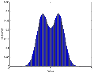
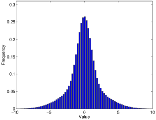
(a)		(b)

Figure 3: Histograms of different Gaussian mixture ensembles. (a) Ensemble A: a bimodal ensemble with $(\nu_{0},\sigma^{2}_{0})=(-1,0.5)$ and $(\nu_{1},\sigma^{2}_{1})=(1,0.5)$. (b) Ensemble B: mimics a heavy-tailed distribution, with $(\nu_{0},\sigma^{2}_{0})=(0,1)$ and $(\nu_{1},\sigma^{2}_{1})=(0,9)$.

Here we show results for a 2-D grid with $N=64$ nodes. Since the mixture variables have $m=2$ states, the coupling distribution can be written as

$$p(x\,;\,{\theta^{*}})\propto\exp\big{\{}\sum_{s\in V}\theta^{*}_{s}x_{s}+\sum_{(s,t)\in E}\theta^{*}_{st}x_{s}x_{t}\big{\}},$$

where $x\in\{-1,+1\}^{N}$ are “spin” variables indexing the mixture components. In all trials, we chose $\theta^{*}_{s}=0$ for all nodes $s\in V$, which ensures uniform marginal distributions $p(x_{s}\,;\,{\theta^{*}})=[0.5\;\;0.5]^{T}$ at each node. We tested two types of coupling in the underlying Markov random field:

1. In the case of attractive coupling, for each coupling strength $\gamma\in[0,1]$, we chose edge parameters as $\theta^{*}_{st}\sim\mathcal{U}[0,\gamma]$.

2. In the case of mixed coupling, for each coupling strength $\gamma\in[0,1]$, we chose edge parameters as $\theta^{*}_{st}\sim\mathcal{U}[-\gamma,\gamma]$.

Here $\mathcal{U}[a,b]$ denotes a uniform distribution on the interval $[a,b]$. In all cases, we varied the SNR parameter $\alpha$, as specified in the observation model (32), in the interval $[0,1]$.

Shown in Figure 4 are 2-D surface plots of the average percentage increase in MSE, taken over 100 trials, as a function of the coupling strength $\gamma\in[0,1]$ and the observation SNR parameter $\alpha\in[0,1]$ for the independence model (left column), BP approach (middle column) and TRW method (right column). The top two rows show performance for attractive coupling, for mixture ensemble A ((a) through (c)) and ensemble B ((d) through (f)), whereas the bottom two row show performance for mixed coupling, for mixture ensemble A ((g) through (i)) and ensemble B ((j) through (l)).

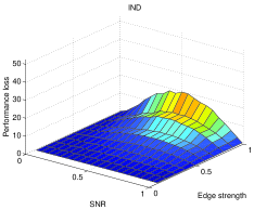
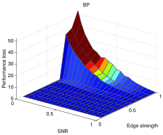
(a)	(b)	(c)
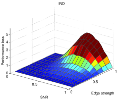
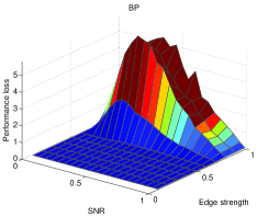
(d)	(e)	(f)
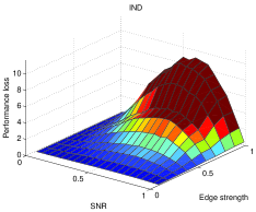
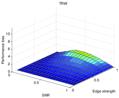
(g)	(h)	(i)
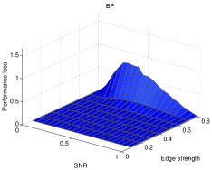
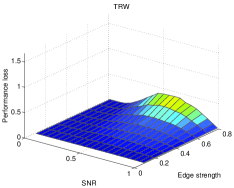
(j)	(k)	(l)

Figure 4: Surface plots of the percentage increase in MSE relative to Bayes optimum for different methods as a function of observation SNR for grids with $N=64$ nodes. Left column: independence model (IND). Center column: ordinary belief propagation (BP). Right column: tree-reweighted algorithm (TRW). First row: Attractive coupling and a Gaussian mixture with components $(\nu_{0},\sigma^{2}_{0})=(-1,0.5)$ and $(\nu_{1},\sigma^{2}_{1})=(1,0.5)$. Second row: Attractive coupling and a Gaussian mixture with components $(\nu_{0},\sigma^{2}_{0})=(0,1)$ and $(\nu_{0},\sigma^{2}_{1})=(0,9)$. Third row: Mixed coupling and a Gaussian mixture with components $(\nu_{0},\sigma^{2}_{0})=(-1,0.5)$ and $(\nu_{1},\sigma^{2}_{1})=(1,0.5)$. Fourth row: Mixed coupling and a Gaussian mixture with components $(\nu_{0},\sigma^{2}_{0})=(0,1)$ and $(\nu_{0},\sigma^{2}_{1})=(0,9)$.

First, observe that for weakly coupled problems ($\gamma\approx 0$), whether attractive or mixed coupling, all three methods—including the independence model—perform quite well, as should be expected given the weak dependency between different nodes in the Markov random field. Although not clear in these plots, the standard BP method outperforms the TRW-based method for weak coupling; however, both methods lose than than 1% in this regime. As the coupling is increased, the BP method eventually deteriorates quite seriously; indeed, for large enough coupling and low/intermediate SNR, its performance can be worse than the independence (IND) model. This deterioration is particularly severe for the case of mixture ensemble A with attractive coupling, where the percentage loss in BP can be as high as 50%. Looking at alternative models (in which phase transitions are known), we have found that this type of rapid degradation coincides with the appearance of multiple fixed points. In contrast, the behavior of the TRW method is extremely stable, which is consistent with our theoretical results.

7.3 Comparison between theory and practice

We now compare the practical behavior of the tree-reweighted sum-product algorithm to the theoretical predictions from Theorem 1. In general, we have found that in quantitative terms, the bounds (41) are rather conservative—in particular, the TRW sum-product method performs much better than the bounds would predict. However, here we show how the bounds can capture qualitative aspects of the MSE increase in different regimes.

Figure 5 provides plots of the actual MSE increase for the TRW algorithm (dotted blue lines), compared to the theoretical bound (41) (solid red lines), for the grid with $N=64$ nodes, and attractive coupling of strength $\gamma=0.70$. For all comparisons in both panels, we used $L=0.10$, which numerical calculations showed to be a reasonable choice for this coupling strength. (Overall, changes in the constant $L$ primarily cause the bounds to shift up and down on the log scale, and so do not overly affect the qualitative comparisons given here.)

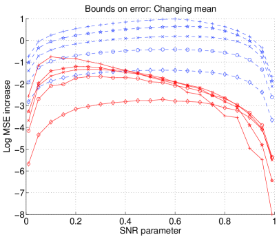
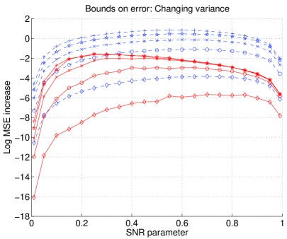
(a)	(b)

Figure 5: Comparison of actual MSE increase and upper bounds for grid with $N=64$ nodes with attractive coupling. (a) Equal variances $\sigma_{0}^{2}=\sigma_{1}^{2}=0.5$, and mean vectors $(\nu_{0},\nu_{1})$ ranging from $(-0.5,0.5)$ to $(-2.5,2.5)$. (b) Equal mean vectors $\nu_{0}=\nu_{1}=0$, and variances $(\sigma_{0}^{2},\sigma_{1}^{2})$ ranging from $(1,1.25)$ to $(1,25)$.

Panel (a) provides the comparison ensembles of type A, with fixed variances $\sigma^{2}_{0}=\sigma^{2}_{1}=0.5$ and mean vectors $(\nu_{0},\nu_{1})$ ranging from $(-0.5,0.5)$ to $(-2.5,2.5)$. Note how the bounds capture the qualitative behavior for low SNR, for which the difficulty of the problem increases as the mean separation is increased. In contrast, in the high SNR regime, the bounds are extremely conservative, and fail to predict that the sharp drop-off in error as the SNR parameter $\alpha$ approaches one. This drop-off is particularly pronounced for the ensemble with largest mean separation (marked with $+$). Panel (b) provides a similar comparison for ensembles of type B, with fixed mean vectors $\nu_{0}=\nu_{1}=0$, and variances $(\sigma^{1}_{0},\sigma^{2}_{1})$ ranging from $(1,1.25)$ to $(1,25)$. In this case, although the bounds are still very conservative in quantitative terms, they reasonably capture the qualitative behavior of the error over the full range of SNR.

8 Discussion

Key challenges in the application of Markov random fields include the estimation (learning) of model parameters, and performing prediction using noisy samples (e.g., smoothing, interpolation, denoising). Both of these problems present substantial computational challenges for general Markov random fields. In this paper, we have described and analyzed methods for joint estimation and prediction that are based on convex variational methods. Our central result is that using inconsistent parameter estimators can be beneficial in the computation-limited setting. Indeed, our results provide rigorous confirmation of the fact that using parameter estimates that are “systematically incorrect” is helpful in offsetting the error introduced by using an approximate method during the prediction step. In concrete terms, we demonstrated that a joint prediction/estimation method using the tree-reweighted sum-product algorithm yields good performance across a wide range of experimental conditions. Although our work has focused on a particular scenario, we suspect that similar ideas and techniques will be useful in related applications of approximate methods for learning and prediction.

Acknowledgments

This work was supported by an Alfred P. Sloan Foundation Fellowship, an Okawa Foundation Research Fellowship, an Intel Corporation Equipment Grant, and NSF Grant DMS-0528488.

Appendix A Tree-based relaxation

As an illustration on the single cycle on $3$ vertices, the pseudomarginal vector with elements

$$\tau_{s}(x_{s})=\begin{bmatrix}0.5\\ 0.5\end{bmatrix}\;\;\mbox{for $s=1,2,3$}\quad\mbox{and}\quad\tau_{st}(x_{s},x_{t})=\begin{bmatrix}\alpha_{st}&0.5-\alpha_{st}\\ 0.5-\alpha_{st}&\alpha_{st}\end{bmatrix}$$

belongs to $\operatorname{LOCAL}_{\phi}(G)$ for all choices $\alpha_{st}\in[0,0.5]$, but fails to belong to $\operatorname{MARG}_{\phi}(G)$, for instance, when $\alpha_{12}=\alpha_{23}=\alpha_{13}=0$.

Appendix B Proof of Lemma 2

Using Lemma 1 and the mean value theorem, we write

$$\mu(\theta+\delta)-\mu(\theta) = \nabla A(\theta+\delta)-\nabla A(\theta)$$

$$= \nabla^{2}A(\theta+t\delta)\delta$$

for some $t\in(0,1)$. Hence, it suffices to show that the eigenspectrum of the Hessian $\nabla^{2}A(\theta)=\operatorname{cov}_{\theta}\{\phi(X)\}$ is uniformly bounded above by $L<+\infty$. The functions $\phi$ are all 0-1 valued indicator functions, so that the diagonal elements of $\operatorname{cov}_{\theta}\big{\{}\phi(X)\big{\}}$ are bounded above—in particular, $\operatorname{var}(\phi_{\alpha}(X))\leq\frac{1}{4}$ for any index $\alpha\in\{1,\ldots,d\}$. Consequently, we have

$$\lambda_{\operatorname{max}}(\operatorname{cov}_{\theta}\{\phi(X)\}) \leq \sum_{\alpha=1}^{d}\lambda_{\alpha}(\operatorname{cov}_{\theta}\{\phi(X)\}\;=\;\operatorname{trace}(\operatorname{cov}_{\theta}\{\phi(X)\}\;=\;\frac{d}{4}$$

as required.

Appendix C Proof of Lemma 3

Consider a spanning tree $T$ of $G$ with edge set $E(T)$. Given a vector $\tau\in\operatorname{LOCAL}_{\phi}(G)$, we associate with $T$ a subvector $\tau(T)$ formed by those components of $\tau$ associated with vertices $V$ and edges $E(T)$. Note that by construction $\tau(T)\in\operatorname{LOCAL}_{\phi}(T)=\operatorname{MARG}_{\phi}(T)$. The mapping $\tau\mapsto\tau(T)$ can be represented by a projection matrix $\Pi^{T}\in{\mathbb{R}}^{d(T)\times d}$ with the block structure

$$\Pi^{T}:=\begin{bmatrix}I_{d(T)\times d(T)}&0_{d(T)\times(d-d(T))}\end{bmatrix}.$$

In this definition, we are assuming for convenience that $\tau$ is ordered such that the $d(T)$ components corresponding to the tree $T$ are placed first. With this notation, we have $\Pi^{T}\tau=\begin{bmatrix}\tau(T)&0\end{bmatrix}^{\prime}$.

By our construction of the function $B_{\rho}$, there exists a probability distribution $\mathbf{\rho}:=\{\rho(T)\;|\;T\in\mathfrak{T}\}$ such that $B_{\rho}(\tau)=\sum_{T\in\mathfrak{T}}\rho(T)A^{*}(\tau(T))$, where $A^{*}(\tau(T))$ denotes the negative entropy of the tree-structured distribution defined by the vector of marginals $\tau(T)$. Hence, the Hessian of $B_{\rho}$ has the decomposition

$$\nabla^{2}B_{\rho}(\tau) = \sum_{T\in\mathfrak{T}}\rho(T)(\Pi^{T})^{\prime}\,\nabla^{2}A^{*}(\tau(T))(\Pi^{T})$$ (48)

To check dimensions of the various quantities, note that $\nabla^{2}A^{*}(\tau(T))$ is a $d(T)\times d(T)$ matrix, and recall that each matrix $\Pi^{T}\in{\mathbb{R}}^{d(T)\times d}$.

Now by Lemma 2, the eigenvalues of the $\nabla^{2}A$ are uniformly bounded above; hence, the eigenvalues of $\nabla^{2}A^{*}$ are uniformly bounded away from zero. Hence, for each tree $T$, there exists a constant $C_{T}$ such that for all $z\in{\mathbb{R}}^{d}$

$$z^{\prime}(\Pi^{T})^{\prime}\,\nabla^{2}A^{*}(\tau(T))(\Pi^{T})z\;\geq\;C_{T}\|\Pi^{T}z\|^{2}\;=\;C_{T}\|z\{T\}\|^{2}.$$

Substituting this relation into our decomposition (48) and expanding the sum over $T$ yields

$$z^{\prime}\nabla^{2}B_{\rho}(\tau)z \geq \sum_{T\in\mathfrak{T}}\rho(T)C_{T}\|z\{T\}\|^{2}$$ (49)

$$= \big{[}\sum_{T\in\mathfrak{T}}\rho(T)C_{T}\big{]}\sum_{s\in V}\|z\{s\}\|^{2}+\sum_{(s,t)\in E}\big{[}\sum_{T\in\mathfrak{T}}\rho(T)C_{T}\mathbb{I\,}[(s,t)\in E(T)]\;\big{]}\;\|z\{(s,t)\}\|^{2}.\qquad$$

Defining $C^{*}:=\min_{T\in\mathfrak{T}}C_{T}$, we have the lower bounds

$$\big{[}\sum_{T\in\mathfrak{T}}\rho(T)C_{T}\big{]} \geq C^{*}\sum_{T\in\mathfrak{T}}\rho(T)\;=\;C^{*}\;>\;0$$

$$\sum_{T\in\mathfrak{T}}\rho(T)C_{T}\mathbb{I\,}[(s,t)\in E(T)] \geq C^{*}{T\in\mathfrak{T}}\rho(T)\mathbb{I\,}[(s,t)\in E(T)]\;=\;C^{*}\rho_{st}\;\geq\;C^{*}\rho^{*}>0,$$

where $\rho^{*}:=\min\limits_{(s,t)\in E}\rho_{st}>0$. Applying these bounds to equation (49) yields the final inequality

$$z^{\prime}\nabla^{2}B_{\rho}(\tau)z \geq C^{*}\rho^{*}\|z\|^{2}\quad\forall z\in{\mathbb{R}}^{d}$$ (50)

with $C^{*}\rho^{*}>0$, which establishes that the eigenvalues of $\nabla^{2}B_{\rho}(\tau)$ are bounded away from zero.

Appendix D Form of exponential parameter

Consider the observation model $y_{s}=\alpha z_{s}+\sqrt{1-\alpha^{2}}v_{s}$, where $v_{s}\sim N(0,1)$ and $z_{s}$ is a mixture of two Gaussians $(\nu_{0},\sigma^{2}_{0})$ and $(\nu_{1},\sigma^{2}_{1})$. Conditioned on the value of the mixing indicator $X_{s}=j$, the distribution of $y_{s}$ is Gaussian with mean $\alpha\nu_{j}$ and variance $\alpha^{2}\sigma^{2}_{j}+(1-\alpha^{2})$.

Let us focus on one component $p(y_{s}\,|\,x_{s})$ in the factorized conditional distribution $p(y\,|\,x)=\prod_{s=1}^{n}p(y_{s}\,|\,x_{s})$. For $j=0,1$, it has the form

$$p(y_{s}\,|\,X_{s}=j) = \frac{1}{\sqrt{2\pi\big{[}\alpha^{2}\sigma^{2}_{j}+(1-\alpha^{2})\big{]}}}\exp\Big{\{}-\frac{1}{2\big{[}\alpha^{2}\sigma^{2}_{j}+(1-\alpha^{2})\big{]}}(y_{s}-\alpha\nu_{j})^{2}\Big{\}}.$$ (51)

We wish to represent the influence of this term on $x_{s}$ in the form $\exp(\gamma_{s}x_{s})$ for some exponential parameter $\gamma_{s}$. We see that $\gamma_{s}$ should have the form

$$\gamma_{s} = \log p(y_{s}\,|\,X_{s}=1)-\log p(y_{s}\,|\,X_{s}=0)$$

$$= \frac{1}{2}\log\frac{\big{[}\alpha^{2}\sigma^{2}_{0}+(1-\alpha^{2})\big{]}}{\big{[}\alpha^{2}\sigma^{2}_{1}+(1-\alpha^{2})\big{]}}+\frac{(y_{s}-\alpha\nu_{0})^{2}}{2\big{[}\alpha^{2}\sigma^{2}_{0}+(1-\alpha^{2})\big{]}}-\frac{(y_{s}-\alpha\nu_{1})^{2}}{2\big{[}\alpha^{2}\sigma^{2}_{1}+(1-\alpha^{2})\big{]}}$$

References

- [1] A. Benveniste, M. Metivier, and P. Priouret. Adaptive Algorithms and Stochastic Approximations. Springer-Verlag, New York, NY, 1990.
- [2] D.P. Bertsekas. Nonlinear programming. Athena Scientific, Belmont, MA, 1995.
- [3] J. Besag. Statistical analysis of non-lattice data. The Statistician, 24(3):179–195, 1975.
- [4] J. Besag. Efficiency of pseudolikelihood estimation for simple Gaussian fields. Biometrika, 64(3):616–618, 1977.
- [5] L.D. Brown. Fundamentals of statistical exponential families. Institute of Mathematical Statistics, Hayward, CA, 1986.
- [6] M.S. Crouse, R.D. Nowak, and R.G. Baraniuk. Wavelet-based statistical signal processing using hidden Markov models. IEEE Trans. Signal Processing, 46:886–902, April 1998.
- [7] M. Deza and M. Laurent. Geometry of Cuts and Metric Embeddings. Springer-Verlag, New York, 1997.
- [8] W. T. Freeman, E. C. Pasztor, and O. T. Carmichael. Learning low-level vision. Intl. J. Computer Vision, 40(1):25–47, 2000.
- [9] W. T. Freeman and Y. Weiss. On the optimality of solutions of the max-product belief propagation algorithm in arbitrary graphs. IEEE Trans. Info. Theory, 47:736–744, 2001.
- [10] T. Heskes, K. Albers, and B. Kappen. Approximate inference and constrained optimization. In Uncertainty in Artificial Intelligence, volume 13, pages 313–320, July 2003.
- [11] A. Ihler, J. Fisher, and A. S. Willsky. Loopy belief propagation: Convergence and effects of message errors. Journal of Machine Learning Research, 6:905–936, May 2005.
- [12] S. L. Lauritzen. Graphical Models. Oxford University Press, Oxford, 1996.
- [13] M. A. R. Leisink and H. J. Kappen. Learning in higher order Boltzmann machines using linear response. Neural Networks, 13:329–335, 2000.
- [14] J. S. Liu. Monte Carlo strategies in Scientific Computing. Springer-Verlag, New York, NY, 2001.
- [15] T. P. Minka. A family of algorithms for approximate Bayesian inference. PhD thesis, MIT, January 2001.
- [16] T. Richardson and R. Urbanke. The capacity of low-density parity check codes under message-passing decoding. IEEE Trans. Info. Theory, 47:599–618, February 2001.
- [17] B. D. Ripley. Spatial statistics. Wiley, New York, 1981.
- [18] C. P. Robert and G. Casella. Monte Carlo statistical methods. Springer-Verlag, New York, NY, 1999.
- [19] G. Rockafellar. Convex Analysis. Princeton University Press, Princeton, 1970.
- [20] M. Ross and L. P. Kaebling. Learning static object segmentation from motion segmentation. In 20th National Conference on Artificial Intelligence, 2005.
- [21] P. Rusmevichientong and B. Van Roy. An analysis of turbo decoding with Gaussian densities. In NIPS 12, pages 575–581. MIT Press, 2000.
- [22] C. Sutton and A. McCallum. Piecewise training of undirected models. In Uncertainty in Artificial Intelligence, July 2005.
- [23] S. Tatikonda. Convergence of the sum-product algorithm. In Information Theory Workshop, April 2003.
- [24] S. Tatikonda and M. I. Jordan. Loopy belief propagation and Gibbs measures. In Proc. Uncertainty in Artificial Intelligence, volume 18, pages 493–500, August 2002.
- [25] Y. W. Teh and M. Welling. On improving the efficiency of the iterative proportional fitting procedure. In Workshop on Artificial Intelligence and Statistics, 2003.
- [26] D. M. Titterington, A.F.M. Smith, and U.E. Makov. Statistical analysis of finite mixture distributions. Wiley, New York, 1986.
- [27] M. J. Wainwright, T. S. Jaakkola, and A. S. Willsky. Tree-based reparameterization framework for analysis of sum-product and related algorithms. IEEE Trans. Info. Theory, 49(5):1120–1146, May 2003.
- [28] M. J. Wainwright, T. S. Jaakkola, and A. S. Willsky. Tree-reweighted belief propagation algorithms and approximate ML estimation by pseudomoment matching. In Workshop on Artificial Intelligence and Statistics, January 2003.
- [29] M. J. Wainwright, T. S. Jaakkola, and A. S. Willsky. A new class of upper bounds on the log partition function. IEEE Trans. Info. Theory, 51(7):2313–2335, July 2005.
- [30] M. J. Wainwright and M. I. Jordan. Graphical models, exponential families, and variational inference. Technical report, UC Berkeley, Department of Statistics, No. 649, September 2003.
- [31] M. J. Wainwright and M. I. Jordan. Log-determinant relaxation for approximate inference in discrete Markov random fields. Accepted to IEEE Trans. Signal Processing, June 2005.
- [32] M. J. Wainwright and M. I. Jordan. A variational principle for graphical models. In New Directions in Statistical Signal Processing. MIT Press, Cambridge, MA, 2005.
- [33] Y. Weiss. Correctness of local probability propagation in graphical models with loops. Neural Computation, 12:1–41, 2000.
- [34] W. Wiegerinck. Approximations with reweighted generalized belief propagation. In Workshop on Artificial Intelligence and Statistics, January 2005.
- [35] J.S. Yedidia, W. T. Freeman, and Y. Weiss. Constructing free energy approximations and generalized belief propagation algorithms. IEEE Trans. Info. Theory, 51(7):2282–2312, July 2005.
- [36] L. Younes. Estimation and annealing for Gibbsian fields. Ann. Inst. Henri Poincare, 24(2):269–294, 1988.