Low-Density Parity-Check Code with Fast Decoding Speed

Abstract

Low-Density Parity-Check (LDPC) codes received much attention recently due to their capacity-approaching performance. The iterative message-passing algorithm is a widely adopted decoding algorithm for LDPC codes [7]. An important design issue for LDPC codes is designing codes with fast decoding speed while maintaining capacity-approaching performance. In another words, it is desirable that the code can be successfully decoded in few number of decoding iterations, at the same time, achieves a significant portion of the channel capacity. Despite of its importance, this design issue received little attention so far. In this paper, we address this design issue for the case of binary erasure channel.

We prove that density-efficient capacity-approaching LDPC codes satisfy a so called “flatness condition”. We show an asymptotic approximation to the number of decoding iterations. Based on these facts, we propose an approximated optimization approach to finding the codes with good decoding speed. We further show that the optimal codes in the sense of decoding speed are “right-concentrated”. That is, the degrees of check nodes concentrate around the average right degree.

I Introduction

Low-Density Parity-Check (LDPC) codes are generally decoded by the iterative message-passing algorithm [7]. An important design issue is finding the codes with fast decoding speed while maintaining good capacity-approaching performance. That is, the bit error rate approaches zero with few decoding iterations while a significant fraction of channel capacity is achieved. Such codes are desirable because they have less decoding computational complexity and delay.

Despite of its importance, this design issue received little attention so far. In this paper, we address this design issue for the case of Binary Erasure Channel (BEC). BEC is widely adopted as a practical channel model for packet network communications. In addition, previous research has shown that the insights gained from the case of BEC can generally be carried over to the cases of many other channels.

“Density Evolution” (DE) is an asymptotic analysis method for LDPC code performance under the message-passing decoding [5]. DE iteratively calculates the probability distributions of messages for the case where the codeword length is infinity. For a code with sufficiently long codeword length, the corresponding distributions of messages are close to these of the infinitely long codes. Hence, the code performances can be approximately determined, such as, bit error rates or message erasure probabilities in the case of BEC.

Given that the message erasure probabilities can be approximately calculated, a brutal force approach to finding LDPC codes with good decoding speed is solving a constraint optimization problem. The optimization variables are the code parameters. The objective function is the number of decoding iterations, which can be approximated calculated by DE. And the constraints includes the fixed code rate, the condition ensuring that the code can be successfully decoded, and the valid ranges of the code parameters.

Although the above brutal force approach can yield certain codes with good decoding speed, it is not satisfactory due to the following reasons. First, the constraint optimization problem does not have nice numerical properties. The objective function is discrete and indifferentiable. Almost all optimization algorithms have convergence problems. It is numerically difficult to find the optimal solutions. Second, the approach does not provide a closed-form relation between the number of iterations and the code parameters. Therefore, we can not gain any insight into the problem.

We propose an alternative and tractable approach in this paper. We prove that “density-efficient” and “capacity-approaching” LDPC codes satisfy a so called “flatness condition”. By “capacity-approaching”, we mean that the code rate is close to the channel capacity. By “density-efficient”, we mean that the density of the parity-check matrix is low. In this paper, we only consider codes with efficiently low parity-check matrix density and low maximal left and right degrees. The codes with high parity-check matrix density or high maximal degrees are not practical in implementations.

The flatness-condition simplify our discussion on decoding speed. Based on that, we present an asymptotic approximation to the number of decoding iterations. The asymptotic approximation yields an approximated optimization approach to designing codes with good decoding speed. Instead of minimizing the number of decoding iterations directly, the approximated optimization approach minimizes the asymptotic approximation. Numerical results confirm that the number of decoding iterations and its asymptotic approximation are consistent. The approximated optimization approach also has better numerical properties. The convergence problem in the brutal force approach is avoided.

The asymptotic approximation provides a closed-form relation between the number of decoding iterations and the code parameters. Hence, it provides useful insights into the design problem. One part of the discussion in this paper on optimal degree distributions in the sense of decoding speed is based on this closed-form relation. We also anticipate that this closed-form relation will facilitate further discussion on decoding speed in the future.

We also discuss the conditions for the optimal degree distributions in the sense of decoding speed. We show that the optimal codes are “right-concentrated”. That is, the degrees of check nodes concentrate around the average right degree. In previous research, several such degree distributions are numerically found to have nice performance

The remainder of this paper is organized as follows. In Section II, we review LDPC codes, the message-passing decoding, “density evolution”, and the density capacity-approaching tradeoff. Readers who are familiar with these materials, can skip this section. In Section III, we discuss the flatness condition and asymptotic approximation to the number of decoding iterations. In Section IV, we discuss the proposed approximated optimization approach for finding codes with good decoding speed. In Section V, we discuss the conditions for optimal degree distributions in the sense of decoding speed. In Section VI, we show several numerical examples. In Section VII, we present our conclusions.

II Preliminary

II-A Binary Erasure Channel

Figure 1: The Binary Erasure Channel

A BEC is shown in Fig. 1. The channel takes binary inputs and outputs $0$, $1$, or $e$, where $e$ stands for an erasure. The transmitted binary signal is received correctly with probability $1-\xi$. Otherwise, the channel outputs an erasure. The probability $\xi$ is called the channel parameter. The channel capacity $C=1-\xi$.

II-B LDPC code

LDPC codes are linear block codes with sparse parity-check matrix. The codes can be represented by Tanner graphs. A Tanner graph is a bipartite graph. One of its partition consists of variable nodes; whereas the other partition consists of check nodes. Each variable node represents one codeword bit; while each check node represent one linear check. A Tanner graph is shown in Fig. 2. The variable nodes are drawn as circles; whereas the check nodes are drawn as squares.

Figure 2: The Tanner graph representation of Low-Density Parity-Check codes

In this paper, we consider randomly generated LDPC codes. The Tanner graph is generated according to the three code parameters: the left degree distribution $\lambda(x)$, the right degree distribution $\rho(x)$, and the codeword length $N$. The left and right degree distributions are polynomials:

$$\lambda(x)=\sum_{i=2}^{d_{v}}\lambda_{i}x^{i-1}$$ (1)

$$\rho(x)=\sum_{j=2}^{d_{c}}\rho_{j}x^{j-1}$$ (2)

where $\lambda_{i}$ is the fraction of edges connected to variable nodes with degree $i$; while $\rho_{j}$ is the fraction of edges connected to check nodes with degree $j$. The Tanner graph is generated by first growing edges from variable and check nodes according to the degree distributions. The edges from variable nodes and check nodes are then uniformly randomly connected. If the codeword length is sufficiently long, approximately the code rate

$$R=1-\frac{\int_{0}^{1}\rho(x)dx}{\int_{0}^{1}\lambda(x)dx}$$ (3)

II-C Message-passing Decoding

The message-passing algorithm [7] is an iterative decoding algorithm. The algorithm computes likelihood functions for all codeword bits iteratively. The final decoding decisions are hard threshold decisions on the likelihood functions.

In the case of BEC, the likelihood function has a finite alphabet. The message-passing algorithm becomes simple. During each iteration, the algorithm find check nodes with only one neighboring variable node being still erasure. The algorithm then corrects these erasures according to the linear constrains.

II-D Density Evolution

Density Evolution [5] calculates the distributions of messages for the codes with infinitely long codeword length. In the case of BEC, the message erasure probability $P_{e}^{(l)}$ after the $l$-th iteration can be approximately calculated as follows:

$$P_{e}^{(l)}=\xi\lambda(1-\rho(1-P_{e}^{(l-1)}))$$ (4)

Asymptotically with the codeword length, the code can be successfully decoded with high probability if and only if

$$\xi\lambda(1-\rho(1-x))<x\,\,\,\mbox{ for any }x\in(0,\xi]$$ (5)

II-E Density Capacity-approaching Tradeoff

It is shown that LDPC codes with bounded degrees can not achieve the channel capacity. There exists a tradeoff between the parity-check matrix density and the achievable rate [1] [9]. In the case of BEC, Shokrollahi [3] shows the following bound for achievable rate:

$$(1-\xi)^{a}\leq\frac{\Delta R}{\xi+\Delta R}$$ (6)

where, $a$ is the average right degree,

$$1/a=\int_{0}^{1}\rho(x)dx$$ (7)

and $\Delta R$ is the gap between the achievable rate to the channel capacity. This lower bound of the gap to the capacity decreases exponentially as the average degree increases. In the same paper, Shokrollahi show that this bound is tight. That is, there exist codes with an exponentially decreasing gap to the capacity with respect to linearly growing average degrees.

III Flatness Condition and Asymptotic Approximation to the Number of Iterations

In this section, we prove that density-efficient capacity-approaching LDPC codes satisfy a necessary condition - the flatness condition. Based on the flatness condition, we further derive an asymptotic approximation to the number of decoding iterations.

The propositions and lemmas in Section III-B are not meaningful by themselves. They are useful only for proving the main theorems in Section III-C. A reader who is not interesting in the details of the proof can skip the section III-B.

III-A Notation and Definition

Consider a BEC with channel parameter $\xi$. Consider a LDPC code with the left degree distribution $\lambda(x)$ and the right degree distribution $\rho(x)$. Denote the average right degree by $a$. Define $b=1/a$. Let $R$ denote the code rate. The gap between the capacity and the code rate $\Delta R=C-R$. We define the function $B(\Delta R,b,x)$ as follows:

$$B(\Delta R,b,x)=\sqrt{\frac{2\Delta R}{(\xi+\Delta R)(1-\xi)\rho(1-x)}}$$ (8)

We define the decoding convergence time $T_{\eta}$ to be the maximal $l$ such that the message erasure probability is greater than the probability level $\eta$ after $l$ decoding iterations. For any left and right degree distributions $\lambda(x)$ and $\rho(x)$, we define

$$F(\lambda,\rho,\eta)\triangleq\int_{\eta}^{\xi}\frac{1}{x-\xi\lambda(1-\rho(1-x))}dx$$ (9)

Throughout Section III, the derivatives are taken with respect to $x$. Throughout this paper, we also assume that the maximal left and right degrees are upper bounded by $k_{v}a$ and $k_{c}a$ respectively, where $k_{v}$ and $k_{c}$ are constants.

III-B Auxiliary Propositions and Lemmas

The proofs can be found in the Appendices A to H.

Proposition III.1

$$\rho(1-x)\leq(-1)[\rho(1-x)]^{\prime}\leq\frac{k_{c}a}{1-\xi}\rho(1-x),\,\,\,\mbox{ for any }x\in(0,\xi]$$ (10)

Proposition III.2

$$[\rho(1-x)]^{\prime\prime}\leq(-1)\frac{k_{c}a}{1-\xi}[\rho(1-x)]^{\prime},\,\,\,\mbox{ for any }x\in(0,\xi]\$$

Proof:

Similar to that of Proposition 10.

∎

Lemma III.3

$$\int_{0}^{1}\rho(1-x)dx-\int_{0}^{\xi}\left[1-\lambda^{-1}(x/\xi)\right]dx=\frac{b\Delta R}{\xi+\Delta R}$$ (11)

Lemma III.4

$$\frac{1-\lambda^{-1}(x/\xi)}{\rho(1-x)}\geq 1-\sqrt{k_{c}}B(\Delta R,b,x),\,\,\,\mbox{ for any }x\in(0,\xi)$$ (12)

Lemma III.5

$$\left|[\lambda(1-\rho(1-x))]^{\prime\prime}\right|\leq\frac{k_{v}^{2}k_{c}^{2}\rho(1-x)^{2}a^{4}}{(1-\xi)^{2}}+\frac{k_{v}k_{c}^{2}\rho(1-x)a^{3}}{(1-\xi)^{2}}$$ (13)

Lemma III.6

Let $b^{5}+b^{2}<\xi$ and $b^{5}<x<\xi-b^{2}$. Then,

$$\frac{[1-\lambda^{-1}(x/\xi)]^{\prime}}{[\rho(1-x)]^{\prime}}\geq 1+\frac{-k_{c}b}{2(1-\xi)}-\sqrt{k_{c}}B(\Delta R,b,x)(1-\xi)a^{2}$$

$$\frac{[1-\lambda^{-1}(x/\xi)]^{\prime}}{[\rho(1-x)]^{\prime}}\leq 1+\sqrt{k_{c}}B(\Delta R,b,x)a^{5}+\frac{k_{c}b^{4}}{2(1-\xi)}(1+\frac{b^{5}}{1-\xi})^{k_{c}a}$$

Lemma III.7

Let $x_{0}\in(0,\xi)$ and $x_{1}=\xi\lambda(1-\rho(1-x_{0}))$. Then,

$$[\xi\lambda(1-\rho(1-x_{0}))]^{\prime}\leq\frac{[\rho(1-x_{i})]^{\prime}}{[1-\lambda^{-1}(x_{i}/\xi)]^{\prime}}$$ (16)

for $i=0,1$.

Lemma III.8

For $x\in(0,\xi)$,

$$x-\xi\lambda(1-\rho(1-x))\leq\sqrt{\frac{-2b\Delta R}{(\xi+\Delta R)[\rho(1-x)]^{\prime}}}$$ (17)

Lemma III.9

If $b<(1-\xi)/k_{c}$, then

$$\rho(1-\xi+b^{2})\leq\frac{2k_{c}(1-\xi)\Delta R}{(\xi+\Delta R)(1-\xi-k_{c}b^{2})}$$ (18)

III-C Main Theorems

Let us consider a BEC with channel parameter $\xi$. Consider a sequence of degree distribution pairs:

$$(\lambda_{1},\rho_{1}),\cdots,(\lambda_{n},\rho_{n}),\cdots$$ (19)

where

$$\lambda_{n}(x)=\sum_{i}\lambda_{ni}x^{i-1}$$ (20)

$$\rho_{n}(x)=\sum_{j}\rho_{nj}x^{j-1}$$ (21)

are the left and right degree distributions respectively. Each pair of degree distributions defines a code. Let $a_{n}$ denote the average right degree for the $n$-th code. Define $b_{n}=1/a_{n}$. Let $R_{n}$ denote the rate of the $n$-th code. Let $\Delta R_{n}$ denote the gap between the capacity and the code rate for the $n$-th code, $\Delta R_{n}=C-R$.

Then we have the following theorem.

Theorem III.10

If $b_{n}$ is strictly decreasing with $\lim_{n\rightarrow\infty}b_{n}=0$. The gap $\Delta R_{n}$ is strictly decreasing and

$$\lim_{n\rightarrow\infty}\frac{\Delta R_{n}}{(b_{n})^{15}}\rightarrow 0$$ (22)

The successfully decoding condition holds:

$$\xi\lambda_{n}(1-\rho_{n}(1-x))<x,\,\,\,\mbox{for any }x\in(0,\xi]$$ (23)

The maximal degrees of $\lambda_{n}$ and $\rho_{n}$ are upper bounded by $k_{v}a_{n}$ and $k_{c}a_{n}$ respectively, where $k_{v}$ and $k_{c}$ are constants. Then as $n\rightarrow\infty$, the derivative of $\xi\lambda_{n}(1-\rho_{n}(1-x))$ with respect to $x$ converges to $1$ uniformly with respect to $x$ in the interval $(0,\xi]$.

Proof:

The proof is in Appendix I ∎

According to this theorem, the function $\xi\lambda(1-\rho(1-x))$ becomes flat as the code rate approaches the channel capacity and the parity-check matrix density remains efficiently low. Based on this conclusion, we prove the following theorem, which shows an asymptotic approximation to decoding convergence time $T_{\eta}$.

Theorem III.11

Let $\eta$ be a fixed probability level, $0<\eta<\xi$. If $b_{n}$ is strictly decreasing with $\lim_{n\rightarrow\infty}b_{n}=0$. The gap $\Delta R_{n}$ is strictly decreasing and

$$\lim_{n\rightarrow\infty}\frac{\Delta R_{n}}{(b_{n})^{15}}\rightarrow 0$$ (24)

The successfully decoding condition holds:

$$\xi\lambda_{n}(1-\rho_{n}(1-x))<x,\,\,\,\mbox{for any }x\in(0,\xi]$$ (25)

The maximal degrees of $\lambda_{n}$ and $\rho_{n}$ are upper bounded by $k_{v}a_{n}$ and $k_{c}a_{n}$ respectively, where $k_{v}$ and $k_{c}$ are constants. Then as $n\rightarrow\infty$, the ratio

$$F(\lambda_{n},\rho_{n},\eta)/T_{\eta}$$ (26)

goes to $1$.

Proof:

The proof is in Appendix J. ∎

• In the above theorems, we assume that $\Delta R_{n}$ decrease polynomially with respect to $b_{n}$. According to Section II-E, in the most efficient tradeoffs, $\Delta R_{n}$ decreases exponentially with respect to $b_{n}$. We conclude that this condition is generally satisfied in practical applications.

IV Approximated Optimization

A brutal force approach to finding the LDPC code with minimal decoding convergence time $T_{\eta}$ and a fixed gap to the capacity is solving the following constrain optimization problem:

$$\min T_{\eta}$$ (27)

subject to

$$\xi\lambda(1-\rho(1-x))<x\mbox{ for }x\in(0,\xi]$$ (28)

$$\frac{\int_{0}^{1}\rho(x)dx}{\int_{0}^{1}\lambda(x)dx}=1-C+\Delta R$$ (29)

$$\sum_{i}\lambda_{i}=1,\,\,\,\sum_{j}\rho_{j}=1,\,\,\,\lambda_{i}\geq 0,\mbox{ and }\rho_{j}\geq 0$$ (30)

Where $C$ is the channel capacity, and $0<\Delta R<C$ is a fixed gap to the channel capacity. The condition in Eqn. 28 is the successful decoding condition. The condition in Eqn. 29 imposes that the code rate is $C-\Delta R$. The constraints in Eqn. 30 come from the probability nature of degree distributions.

However, the above optimization problem is not tractable. The objective function $T_{\eta}$ is not differentiable. This brings in convergence problems for optimization algorithms. To get around these difficulties, at this point, we invoke Theorem III.11 and replace $T_{\eta}$ by $F(\lambda,\rho,\eta)$. This yields the following approximated optimization problem:

$$\min F(\lambda,\rho,\eta)$$ (31)

subject to

$$\xi\lambda(1-\rho(1-x))<x,\,\,\,\mbox{ for }x\in(0,\xi]$$ (32)

$$\frac{\int_{0}^{1}\rho(x)dx}{\int_{0}^{1}\lambda(x)dx}=1-C+\Delta R$$ (33)

$$\sum_{i}\lambda_{i}=1,\,\,\,\sum_{j}\rho_{j}=1,\,\,\,\lambda_{i}\geq 0,\mbox{ and }\rho_{j}\geq 0$$ (34)

The numerical results confirm that the approximated optimization has nice numerical properties.

V Optimal Degree Distribution

In this section, we discuss the conditions for the optimal degree distributions in the sense of convergence speed. We show that the optimal codes are right-concentrated.

V-A Low Erasure Probability Region Convergence Speed Analysis

In practical applications, the probability level $\eta$ is generally small. The number of decoding iterations while the erasure probability is in a low erasure probability region may constitute a large fraction of the decoding convergence time. That is, the decoding speed in the low erasure probability region dominates the overall decoding speed.

We show in this section that if the average right degree is fixed, then the right-concentrated degree distributions have optimal decoding speed in the low erasure probability region.

Figure 3: The iteration process of erasure probabilities

Note that the relation between $P_{e}^{(l)}$ and $P_{e}^{(l+1)}$ can be also written as follows:

$$y=\rho(1-P_{e}^{(l)})$$ (35)

$$y=1-\lambda^{-1}(P_{e}^{(l+1)}/\xi)$$ (36)

where $y$ is a auxiliary variable. The iterative process of $P_{e}^{(l)}$ is illustrated in Fig. 3. To increase the decoding speed, we need to move the curve $\rho(1-x)$ upward and the curve $1-\lambda^{-1}(x/\xi)$ to the left. Moving the curve $\rho(1-x)$ upward is equivalent to making the function $\rho(1-x)$ larger. Moving the curve $1-\lambda^{-1}(x/\xi)$ to the left is equivalent to making the function $\lambda(1-x)$ smaller. To have fast decoding speed in the low message erasure probability region, we need to make $\rho(x)$ large for $x$ near $1$ and $\lambda(x)$ small for $x$ near $0$.

We need the following auxiliary lemma for proving the main theorem in this section.

Lemma V.1

Let $\gamma(x)$ be a degree distribution with average degree $a$ and maximal degree $d\geq 3$. Assume $\gamma_{i}>0$ and $\gamma_{i+2}>0$, for $1<i<d$. Then another degree distribution $\hat{\gamma}(x)$ with the same average and maximal degrees can be constructed as follows:

$$\hat{\gamma}(x)= {\gamma(x)+\beta x^{i}-\left\{\frac{i}{2(i+1)}\beta x^{i-1}+\frac{i+2}{2(i+1)}\beta x^{i+1}\right\}}$$

where $\beta$ is a sufficiently small positive real number such that $\hat{\gamma}(x)$ is well defined. We also have

$$\gamma(x)<\hat{\gamma}(x),\,\,\,\mbox{ for }\frac{i}{i+2}<x<1$$ (38)

$$\gamma(x)>\hat{\gamma}(x),\,\,\,\mbox{ for }0<x<\frac{i}{i+2}$$ (39)

Proof:

The proof is in Appendix K. ∎

Theorem V.2

Let $d$ be an positive integer. Let $x$ be an arbitrary real number, $x>1-\frac{2}{d+1}$. Then the degree distribution with average degree $a$ and maximal degree $d$ which maximizes the function $\gamma(x)$ is

$$\gamma(x)=\gamma_{i}x^{i-1}+\gamma_{i+1}x^{i}$$ (40)

where $i=\lfloor a\rfloor$ is the largest integer smaller than $a$.

Proof:

The proof is in Appendix L. ∎

The above Theorems imply that the degree distributions with fast decoding speed at the low erasure probability region are right-concentrated.

V-B Asymptotic Approximation Based Analysis

In this section, we discuss the condition for the optimal degree distributions in the approximated constraint optimization program in Eqn. 31, 32, 33, 34. We have the following theorem, which shows that the optimal degree distributions are right-concentrated.

Theorem V.3

Let $(\lambda^{\ast},\rho^{\ast})$ be the solution of the constrain optimization problem in Eqns. 31, 32, 33, 34 with fixed maximal left degree $d_{v}$ and maximal right degree $d_{c}$. Then

• If $\xi\leq 1-e^{-2/d_{c}}$, then $\rho_{j}^{\ast}$ are non-zero only for two $j$’s.

• If $\xi>1-e^{-2/d_{c}}$, then either

  $$\min_{x\in(1-e^{-2/d_{c}},\xi)}[x-\xi\lambda^{\ast}(1-\rho^{\ast}(1-x))]\rightarrow 0$$ (41)

  as $\eta\rightarrow 0$ or $\rho_{j}^{\ast}$ are non-zero only for two $j$’s when $\eta$ is sufficiently small.

Proof:

The proof is in Appendix M. ∎

VI Numerical Examples

In this section, we show several numerical design examples. We also compare the codes designed by the proposed approach to one well-known class of LDPC codes: the Heavy-tail/Poisson codes [6] [2].

Figure 4: The function $\xi\lambda(1-\rho(1-x))$ in the Example 1

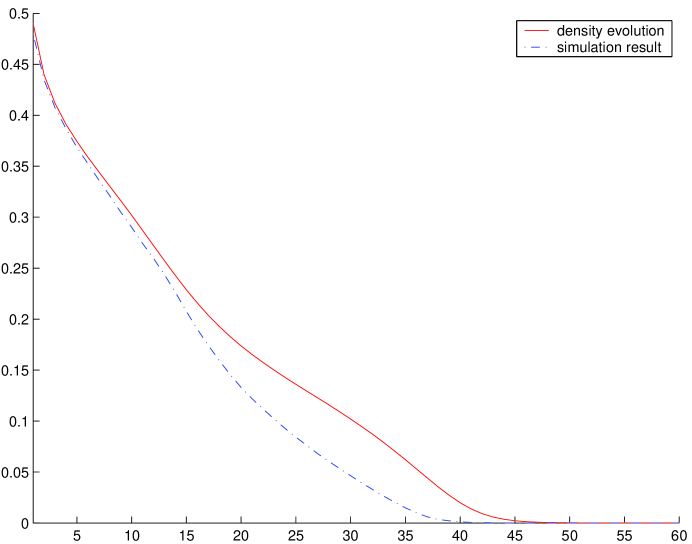
Figure 5: The message erasure probabilities in the example 1

• In this example, we design a LDPC code for a BEC with parameter $\xi=0.48$. The code rate is $0.48$. The left and right degree distributions are as follows:

  $$\lambda(x)=0.1863x+0.4143x^{2}+0.0512x^{8}+0.3482x^{15}$$ (42)

  $$\rho(x)=0.5330x^{6}+0.4670x^{7}$$ (43)

  The function $\xi\lambda(1-\rho(1-x))$ is shown in Fig. 4 as the solid line. The dashed line shows the straight line $y=x$. For $\eta=10^{-3}$, The decoding convergence time $T_{\eta}=47$ in the corresponding density evolution. The asymptotic approximation $F(\lambda,\rho,\eta)=47.9400$.

  We construct practical codes according to the designed degree distributions. The codeword length is $32k$ bits. The simulation results on message erasure probabilities are shown in Fig. 5. The message erasure probabilities after different numbers of iterations are shown as the dash-dot curve. The message erasure probabilities by density evolution are shown as the solid curve.

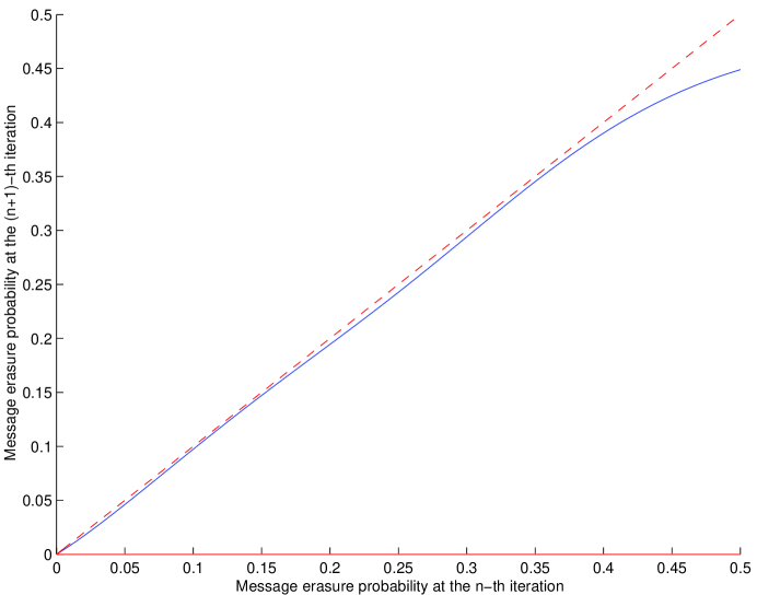
Figure 6: The function $\xi\lambda(1-\rho(1-x))$ in the Example 2

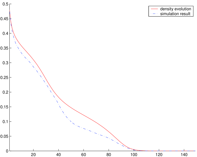
Figure 7: The message erasure probabilities in the Example 2

• In the second example, we consider the BEC with parameter $\xi=0.48$. The code rate is $0.5$. We find the following left and right degree distributions:

  $$\lambda(x)=0.2452x+0.2982x^{2}+0.1112x^{5}+0.3454x^{15}$$ (44)

  $$\rho(x)=0.3398x^{6}+0.6602x^{7}$$ (45)

  The function $\xi\lambda(1-\rho(1-x))$ is shown in Fig. 6 as the solid line. The dash line shows the straight line $y=x$. For $\eta=10^{-3}$, the decoding convergence time $T_{\eta}=107$ in the corresponding density evolution. The asymptotic approximation $F(\lambda,\rho,\eta)=108.7363$.

  We construct practical codes according to the above degree distributions. The simulation results on message erasure probabilities after different numbers of iterations are shown in Fig. 7 as the dash-dot curve. The message erasure probabilities by density evolution are shown as the solid curve. The codeword length is $32k$ bits.

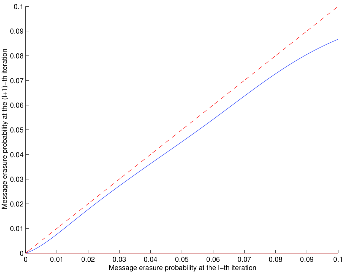
Figure 8: The function $\xi\lambda(1-\rho(1-x))$ in the Example 3

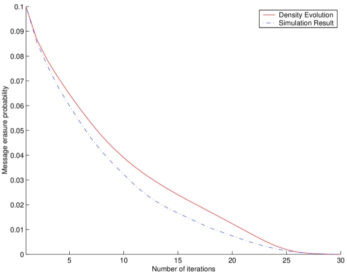
Figure 9: The message erasure probabilities in the Example 3

• In the third example, we design codes for the BEC with parameter $\xi=0.1$. The code rate is $0.885$. The left and right degree distributions are as follows:

  $$\lambda(x)=0.0939x+0.3807x^{2}+0.0443x^{9}+0.1875x^{10}+0.2937x^{31}$$ (46)

  $$\rho(x)=0.4725x^{41}+0.5274x^{42}$$ (47)

  The function $\xi\lambda(1-\rho(1-x))$ is shown in Fig. 8 as the solid curve. The dash line shows the straight line $y=x$. For $\eta=10^{-3}$, the decoding convergence time $T_{\eta}=26$ in the corresponding density evolution. The asymptotic approximation $F(\lambda,\rho,\eta)=26.6844$.

  The simulation results on the message erasure probabilities after different numbers of iterations are shown in Fig. 9. The message erasure probabilities in the density evolution are shown as the solid curve. The codeword length is $32k$ bits.

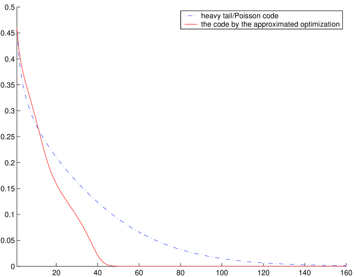
Figure 10: The message erasure probabilities

• In this example, we compare the codes designed by the proposed approach with the Heavy-tail/Possion codes. We consider a BEC with channel parameter $\xi=0.46$. Two codes with half rate and maximal degree $16$ are designed. The left and right degree distributions of the Heavy-tail/Possion codes are as follows [2] :

  $$\lambda(x)= {0.3014x+0.1507x^{2}+0.1005x^{3}+0.0753x^{4}+0.0604x^{5}+}$$

  $${0.0502x^{6}+0.0431x^{7}+0.0377x^{8}+0.0335x^{9}+0.0301x^{10}+}$$

  $${0.0274x^{11}+0.0251x^{12}+0.0232x^{13}+0.0215x^{14}+0.0201x^{15}}$$ (48)

  $$\rho(x)= {0.0060x+0.0213x^{2}+0.0502x^{3}+0.0887x^{4}+0.1255x^{5}+}$$

  $${0.1479x^{6}+0.1495x^{7}+0.1321x^{8}+0.1039x^{9}+0.0735x^{10}+}$$

  $${0.0472x^{11}+0.0278x^{12}+0.0151x^{13}+0.0077x^{14}+0.0036x^{15}}$$ (49)

  The left and right degree distributions by the proposed design approach are as follows:

  $$\lambda(x)=0.1819x+0.4101x^{2}+0.0152x^{7}+0.3928x^{15}$$ (50)

  $$\rho(x)=0.0891x^{6}+0.9109x^{7}$$ (51)

  The decoding convergence time $T_{\eta}$, $\eta=10^{-3}$, is $47$ for the code by the proposed approach and $263$ for the Heavy-tail/Possion codes. The message erasure probabilities of the two codes by density evolution are show in Fig. 10. The dash-dot curve shows the message erasure probabilities for the Heavy-tail/Poisson code. The solid curve shows the message erasure probabilities for the code by the proposed approach.

These numerical results confirm our theoretical results that the derivatives of $\xi\lambda(1-\rho(1-x))$ with respect to $x$ are close to $1$ for density-efficient capacity-approaching codes. The asymptotic approximation $F(\lambda,\rho,\eta)$ is generally tight. The proposed approach yields codes with good decoding speed. The optimal codes are right-concentrated.

VII Conclusions

In this paper, we present a framework for designing LDPC codes with fast decoding speed. Both the theoretical discussion and numerical results show that Density-efficient capacity-approaching codes satisfy the flatness condition. Asymptotically the decoding convergence time $T_{\eta}$ can be approximated by $F(\lambda,\rho,\eta)$. The asymptotic approximation is generally tight for practical scenarios. The optimal degree distributions in the sense of decoding speed are right-concentrated.

Appendix A The proof of Proposition 10

Proof:

The lower bound of $(-1)[\rho(1-x)]^{\prime}$ follows from the fact that

$$(-1)[\rho(1-x)]^{\prime} = \sum_{j=2}^{k_{c}a}\rho_{j}(j-1)(1-x)^{j-2}$$

$$\geq \sum_{j=2}^{k_{c}a}\rho_{j}(1-x)^{j-2}$$

$$\geq \sum_{j=2}^{k_{c}a}\rho_{j}(1-x)^{j-1}=\rho(1-x)$$

Note that the maximal right degree is bounded by $k_{c}a$. The upper bound follows from

$$(-1)[\rho(1-x)]^{\prime} = \sum_{j=2}^{k_{c}a}\rho_{j}(j-1)(1-x)^{j-2}$$ (53)

$$\leq (k_{c}a)\sum_{j=2}^{k_{c}a}\rho_{j}(1-x)^{j-2}$$

$$\leq \frac{k_{c}a}{1-x}\sum_{j=2}^{k_{c}a}\rho_{j}(1-x)^{j-1}$$

$$\leq \frac{k_{c}a}{1-\xi}\sum_{j=2}^{k_{c}a}\rho_{j}(1-x)^{j-1}$$

$$= \frac{k_{c}a}{1-\xi}\rho(1-x)$$

∎

Appendix B The proof of Lemma 11

Proof:

Using the change of variable $x=1-v$, we have

$$\int_{0}^{1}\rho(1-x)dx=\int_{0}^{1}\rho(v)dv=b$$ (54)

Using the change of variable $x=\xi\lambda(u)$, we have

$$\int_{0}^{\xi}\lambda^{-1}(x/\xi)dx=\int_{0}^{1}\xi u\lambda^{\prime}(u)du=\xi-\frac{b\xi}{\xi+\Delta R}$$ (55)

The lemma follows. ∎

Appendix C The Proof of Lemma III.4

Figure 11: The geometrical interpretation of $x_{0}$ and $x_{1}$

Figure 12: The geometrical interpretation

Proof:

Let us denote $x$ by $x_{0}$ for convenience and define

$$c\triangleq 1-\frac{1-\lambda^{-1}(x/\xi)}{\rho(1-x)}$$ (56)

$$x_{1}\triangleq x_{0}-\frac{c\rho(1-x_{0})}{[\rho(1-x_{0})]^{\prime}}$$ (57)

The geometric meaning of $x_{1}$ is shown in Fig. 11. The number $x_{1}$ is the $x$ coordinate of the intersection point of the horizontal line $y=1-\lambda^{-1}(x_{0}/\xi)$ and the straight line tangent to the curve $y=\rho(1-x)$ at the point $(x_{0},\rho(1-x_{0}))$.

The shadowed region in Fig. 11 is smaller than the shadowed region in Fig. 12. The area of the shadowed region in Fig. 11 is

$$\frac{(-1)c^{2}\left[\rho(1-x_{0})\right]^{2}}{2[\rho(1-x_{0})]^{\prime}}$$ (58)

The area of the shadowed region in Fig. 12 is

$$\int_{0}^{1}\rho(1-x)dx-\int_{0}^{\xi}\left[1-\lambda^{-1}(x/\xi)\right]dx=\frac{b\Delta R}{\xi+\Delta R}$$ (59)

Hence

$$c^{2}\leq\frac{-2b\Delta R[\rho(1-x_{0})]^{\prime}}{(\xi+\Delta R)\left[\rho(1-x_{0})\right]^{2}}$$ (60)

We further bound $(-1)[\rho(1-x_{0})]^{\prime}$ as in Proposition 10. This gives us the following bound

$$c\leq\sqrt{\frac{2k_{c}\Delta R}{(\xi+\Delta R)(1-\xi)\rho(1-x_{0})}}$$ (61)

The lemma follows. ∎

Appendix D The Proof of lemma 13

Proof:

We can write $[\lambda(1-\rho(1-x))]^{\prime\prime}$ as follows:

$${[\lambda(1-\rho(1-x))]^{\prime\prime}=}$$

$${\left[\sum_{i=3}^{k_{v}a}\lambda_{i}(i-1)(i-2)\left[1-\sum_{j}\rho_{j}(1-x)^{j-1}\right]^{i-3}\right]\times}$$

$${\left[\sum_{j}\rho_{j}(j-1)(1-x)^{j-2}\right]^{2}-}$$

$${\left[\sum_{i}\lambda_{i}(i-1)\times\left[1-\sum_{j}\rho_{j}(1-x)^{j-1}\right]^{i-2}\right]\times}$$

$${\left[\sum_{j=3}^{k_{c}a}\rho_{j}(j-1)(j-2)(1-x)^{j-3}\right]}$$ (62)

Hence, we have the following bound:

$${\left|[\lambda(1-\rho(1-x))]^{\prime\prime}\right|\leq}$$

$${\left[\sum_{i=3}^{k_{v}a}\lambda_{i}(i-1)(i-2)\left[1-\sum_{j}\rho_{j}(1-x)^{j-1}\right]^{i-3}\right]\times}$$

$${\left[\sum_{j}\rho_{j}(j-1)(1-x)^{j-2}\right]^{2}+}$$

$${\left[\sum_{i}\lambda_{i}(i-1)\times\left[1-\sum_{j}\rho_{j}(1-x)^{j-1}\right]^{i-2}\right]\times}$$

$${\left[\sum_{j=3}^{k_{c}a}\rho_{j}(j-1)(j-2)(1-x)^{j-3}\right]}$$ (63)

Applying the following bounding,

$$(i-1)<k_{v}a$$ (64)

$$(i-2)<k_{v}a$$ (65)

$$(j-1)<k_{c}a$$ (66)

$$(j-2)<k_{c}a$$ (67)

we have

$${\left|[\lambda(1-\rho(1-x))]^{\prime\prime}\right|\leq k_{v}^{2}k_{c}^{2}a^{4}\times}$$

$${\left[\sum_{i=3}^{k_{v}a}\lambda_{i}\left[1-\sum_{j}\rho_{j}(1-x)^{j-1}\right]^{i-3}\right]\left[\sum_{j}\rho_{j}(1-x)^{j-2}\right]^{2}}$$

$${+k_{v}k_{c}^{2}a^{3}\left[\sum_{i}\lambda_{i}\left[1-\sum_{j}\rho_{j}(1-x)^{j-1}\right]^{i-2}\right]}\times$$

$${\left[\sum_{j=3}^{k_{c}a}\rho_{j}(1-x)^{j-3}\right]}$$ (68)

Note that

$$\left[\sum_{i=3}^{k_{v}a}\lambda_{i}\left[1-\sum_{j}\rho_{j}(1-x)^{j-1}\right]^{i-3}\right]\leq 1$$ (69)

$$\left[\sum_{i}\lambda_{i}\left[1-\sum_{j}\rho_{j}(1-x)^{j-1}\right]^{i-2}\right]\leq 1$$ (70)

we have

$${\left|[\lambda(1-\rho(1-x))]^{\prime\prime}\right|\leq k_{v}^{2}k_{c}^{2}a^{4}\left[\sum_{j}\rho_{j}(1-x)^{j-2}\right]^{2}+}$$

$${k_{v}k_{c}^{2}a^{3}\left[\sum_{j=3}^{k_{c}a}\rho_{j}(1-x)^{j-3}\right]}$$ (71)

Further apply the following upper bounds for $\sum_{j}\rho_{j}(1-x)^{j-2}$ and $\sum_{j=3}^{k_{c}a}\rho_{j}(1-x)^{j-3}$

$$\sum_{j}\rho_{j}(1-x)^{j-2}=\frac{\sum_{j}\rho_{j}(1-x)^{j-1}}{1-x}\leq\frac{\rho(1-x)}{1-\xi}$$ (72)

$$\sum_{j=3}^{k_{c}a}\rho_{j}(1-x)^{j-3}\leq\frac{\sum_{j=2}^{k_{c}a}\rho_{j}(1-x)^{j-1}}{(1-x)^{2}}\leq\frac{\rho(1-x)}{(1-\xi)^{2}}$$ (73)

we have

$$\left|[\lambda(1-\rho(1-x))]^{\prime\prime}\right|\leq\frac{k_{v}^{2}k_{c}^{2}\rho(1-x)^{2}a^{4}}{(1-\xi)^{2}}+\frac{k_{v}k_{c}^{2}\rho(1-x)a^{3}}{(1-\xi)^{2}}$$ (74)

∎

Appendix E The Proof of lemma III.6

Proof:

Let $x_{0}\in(b^{5},\xi-b^{2})$. Let $x\in(0,\xi)$, $x\neq x_{0}$, we have the following Taylor series expansion

$${1-\lambda^{-1}(x/\xi)-\rho(1-x)=1-\lambda^{-1}(x_{0}/\xi)-\rho(1-x_{0})+}$$

$${\left\{\left[1-\lambda^{-1}(x_{0}/\xi)\right]^{\prime}-\left[\rho(1-x_{0})\right]^{\prime}\right\}(x-x_{0})+}$$

$${\left\{\left[1-\lambda^{-1}(\zeta/\xi)\right]^{\prime\prime}-\left[\rho(1-\zeta)\right]^{\prime\prime}\right\}\frac{(x-x_{0})^{2}}{2}}$$ (75)

where $\zeta$ is a real number between $x_{0}$ and $x$. According to the hypotheses, $\xi\lambda(1-\rho(1-x))<x$. This implies $1-\lambda^{-1}(x/\xi)-\rho(1-x)<0$, and

$${1-\lambda^{-1}(x_{0}/\xi)-\rho(1-x_{0})+}$$

$${\left\{\left[1-\lambda^{-1}(x_{0}/\xi)\right]^{\prime}-\left[\rho(1-x_{0})\right]^{\prime}\right\}(x-x_{0})+}$$

$${\left\{\left[1-\lambda^{-1}(\zeta/\xi)\right]^{\prime\prime}-\left[\rho(1-\zeta)\right]^{\prime\prime}\right\}\frac{(x-x_{0})^{2}}{2}<0}$$ (76)

Note that $[1-\lambda^{-1}(\zeta/\xi)]^{\prime\prime}>0$, we therefore have the following more convenient inequality:

$${1-\lambda^{-1}(x_{0}/\xi)-\rho(1-x_{0})+}$$

$${\left\{\left[1-\lambda^{-1}(x_{0}/\xi)\right]^{\prime}-\left[\rho(1-x_{0})\right]^{\prime}\right\}(x-x_{0})}$$

$${-\left[\rho(1-\zeta)\right]^{\prime\prime}\frac{(x-x_{0})^{2}}{2}<0}$$ (77)

Set $x=x_{0}+b^{2}$ in the above inequality, with a little algebra we have

$$\left\{\frac{[1-\lambda^{-1}(x_{0}/\xi)]^{\prime}}{[\rho(1-x_{0})]^{\prime}}-1\right\}\geq\frac{b^{2}[\rho(1-\zeta)]^{\prime\prime}}{2[\rho(1-x_{0}]^{\prime}}+\frac{\left[\lambda^{-1}(x_{0}/\xi)+\rho(1-x_{0})-1\right]}{b^{2}[\rho(1-x_{0})]^{\prime}}$$ (78)

To prove the lower bound in the lemma, we will bound the two terms in the right hand side of Eqn. 78 separately.

We bound the first term as follows. Since $[\rho(1-x)]^{\prime\prime}$ is a monotonous decreasing function,

$$[\rho(1-\zeta)]^{\prime\prime}\leq[\rho(1-x_{0})]^{\prime\prime}$$ (79)

Apply the bound in Proposition III.2, we hve

$$[\rho(1-\zeta)]^{\prime\prime}\leq\frac{(-1)k_{c}a}{(1-\xi)}[\rho(1-x_{0})]^{\prime}$$ (80)

Thus, the first term in the right hand side of Eqn. 78 can be lower bounded

$$\frac{b^{2}[\rho(1-\zeta)]^{\prime\prime}}{2[\rho(1-x_{0}]^{\prime}}\geq\frac{-k_{c}b}{2(1-\xi)}$$ (81)

We bound the second term in the right hand side of Eqn. 78 as follows. The second term in the right hand side of Eqn. 78 can be rewritten as follows:

$${\frac{\rho(1-x_{0})-1+\lambda^{-1}(x_{0}/\xi)}{b^{2}[\rho(1-x_{0})]^{\prime}}=}$$

$${(-a^{2})\left\{\frac{\rho(1-x_{0})-1+\lambda^{-1}(x_{0}/\xi)}{\rho(1-x_{0})}\right\}\left\{\frac{\rho(1-x_{0})}{(-1)[\rho(1-x_{0})]^{\prime}}\right\}}$$ (82)

According to Lemma III.4,

$$\frac{\rho(1-x_{0})-1+\lambda^{-1}(x_{0}/\xi)}{\rho(1-x_{0})}\leq\sqrt{k_{c}}B(\Delta R,b,x_{0})$$ (83)

According to Proposition 10

$$\left\{\frac{\rho(1-x_{0})}{-[\rho(1-x_{0})]^{\prime}}\right\}\leq 1$$ (84)

Hence, the second term in the right hand side of Eqn. 78 can be lower bounded as follows.

$$\frac{\rho(1-x_{0})-1+\lambda^{-1}(x_{0}/\xi)}{[\rho(1-x_{0})]^{\prime}b^{2}}\geq-\sqrt{k_{c}}B(\Delta R,b,x)a^{2}$$ (85)

Substituting Eqns. 85 and 81 into Eqn. 78 gives the lower bound in the lemma.

We will prove the upper bound in the lemma. Set $x=x_{0}-b^{5}$ in Eqn. 77, with a little algebra we have

$$\frac{[1-\lambda^{-1}(x_{0}/\xi)]^{\prime}}{[\rho(1-x_{0})]^{\prime}}-1\leq {\frac{1-\lambda^{-1}(x_{0}/\xi)-\rho(1-x_{0})}{b^{5}[\rho(1-x_{0})]^{\prime}}}$$

$${+\frac{-b^{5}[\rho(1-\zeta)]^{\prime\prime}}{2[\rho(1-x_{0})]^{\prime}}}$$ (86)

Since of Lemma III.4 and Proposition 10, the first term at the right hand side of Eqn. 86 can be bounded

$$\frac{1-\lambda^{-1}(x_{0}/\xi)-\rho(1-x_{0})}{[\rho(1-x_{0})]^{\prime}b^{5}}\leq {\frac{a^{5}\sqrt{k_{c}}B(\Delta R,b,x)\rho(1-x_{0})}{(-1)[\rho(1-x_{0})]^{\prime}}}$$

$$\leq {\sqrt{k_{c}}B(\Delta R,b,x)a^{5}}$$ (87)

Note that the maximal right degree is bounded by $k_{c}a$. Hence

$$[\rho(1-\zeta)]^{\prime\prime}\leq {[\rho(1-x_{0})]^{\prime\prime}\left[\frac{1-\zeta}{1-x_{0}}\right]^{k_{c}a-2}}$$

$$\leq {[\rho(1-x_{0})]^{\prime\prime}\left[\frac{1-x_{0}+b^{5}}{1-x_{0}}\right]^{k_{c}a-2}}$$

$$\leq {[\rho(1-x_{0})]^{\prime\prime}\left[1+\frac{b^{5}}{1-\xi}\right]^{k_{c}a}}$$ (88)

By bounding $[\rho(1-\zeta)]^{\prime\prime}$ as in Proposition III.2, the second term at the right hand side of Eqn. 86 can be bounded by

$$(-1)\frac{[\rho(1-\zeta)]^{\prime\prime}b^{5}}{2[\rho(1-x_{0})]^{\prime}}\leq\frac{k_{c}b^{4}}{2(1-\xi)}\left(1+\frac{b^{5}}{1-\xi}\right)^{k_{c}a}$$ (89)

Substituting Eqns. 87 and 89 into Eqn. 86 gives the upper bound in the lemma. ∎

Appendix F The Proof of lemma III.7

Proof:

Notice that

$$[\xi\lambda(1-\rho(1-x_{0}))]^{\prime}=\frac{[\rho(1-x_{0})]^{\prime}}{[1-\lambda^{-1}(x_{1}/\xi)]^{\prime}}$$ (90)

Since $[\rho(1-x)]^{\prime}$ and $[1-\lambda^{-1}(x/\xi)]^{\prime}$ are monotonously increasing,

$$\frac{[\rho(1-x_{1})]^{\prime}}{[1-\lambda^{-1}(x_{1}/\xi)]^{\prime}}\geq\frac{[\rho(1-x_{0})]^{\prime}}{[1-\lambda^{-1}(x_{1}/\xi)]^{\prime}}$$ (91)

$$\frac{[\rho(1-x_{0})]^{\prime}}{[1-\lambda^{-1}(x_{0}/\xi)]^{\prime}}\geq\frac{[\rho(1-x_{0})]^{\prime}}{[1-\lambda^{-1}(x_{1}/\xi)]^{\prime}}$$ (92)

The lemma follows. ∎

Appendix G The Proof of lemma III.8

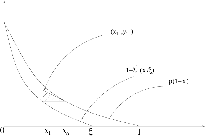
Figure 13: The geometrical interpretation of $x_{0}$ and $x_{1}$.

Proof:

Denote $x$ by $x_{0}$ for convenience. Define

$$x_{1}=\xi\lambda(1-\rho(1-x_{0}))$$ (93)

$$y_{0}=\rho(1-x_{0})$$ (94)

$$y_{1}=y_{0}-(x_{0}-x_{1})[\rho(1-x_{0})]^{\prime}$$ (95)

The geometric meaning of $x_{0}$, $x_{1}$, $y_{0}$, and $y_{1}$ is shown in Fig. 13. The point $(x_{1},y_{1})$ is the intersection of the vertical straight line $x=x_{1}$ and the straight line tangent to the curve $\rho(1-x)$ at the point $(x_{0},y_{0})$.

The area of the shadowed region in Fig. 13 is

$$\frac{-1}{2}[\rho(1-x_{0})]^{\prime}(x_{0}-x_{1})^{2}$$ (96)

The shadowed region in Fig. 13 is smaller than the shadowed region in Fig. 12,

$$\frac{-1}{2}[\rho(1-x_{0})]^{\prime}(x_{0}-x_{1})^{2}\leq\frac{b\Delta R}{\xi+\Delta R}$$ (97)

The lemma follows. ∎

Appendix H The Proof of Lemma III.9

Figure 14: The geometrical interpretation of $x_{1}$

Proof:

Define

$$x_{0}=\xi-b^{2}$$ (98)

$$y_{0}=\rho(1-x_{0})$$ (99)

$$x_{1}=x_{0}+\frac{y_{0}}{(-1)[\rho(1-x_{0})]^{\prime}}$$ (100)

Since $b<(1-\xi)/k_{c}$,

$$x_{1}= {x_{0}+\frac{y_{0}}{(-1)[\rho(1-x_{0})]^{\prime}}\geq x_{0}+\frac{(1-\xi)y_{0}b}{k_{c}\rho(1-x_{0})}}$$

$$\geq {x_{0}+\frac{(1-\xi)b}{k_{c}}>\xi}$$ (101)

The geometric meaning of $x_{1}$ is shown in Fig. 14. The point $(x_{1},0)$ is the intersection of the $x$-axis and the straight line tangent to the curve $y=\rho(1-x)$ at the point $(x_{0},y_{0})$.

The shadowed region in Fig. 14 is smaller than the shadowed region in Fig. 12. For the area of the shadowed triangle region in Fig. 14, the width is $x_{1}-x_{0}$, the height is $(x_{1}-\xi)y_{0}/{x_{1}-x_{0}}$, and the area is

$$\frac{y_{0}(x_{1}-\xi)^{2}}{2(x_{1}-x_{0})}$$ (102)

Since this area is monotonously increase with respect to $x_{1}$, applying the bound for $x_{1}$ in Eqn. H, we have the following lower bound of the area

$$\frac{y_{0}b}{2k_{c}(1-\xi)}\left(1-\xi-k_{c}b\right)^{2}$$ (103)

This lower bound is less than the area of the shadowed region in Fig. 12

$$\frac{y_{0}b}{2k_{c}(1-\xi)}\left(1-\xi-k_{c}b\right)^{2}\leq\frac{b\Delta R}{\xi+\Delta R}$$ (104)

The lemma follows. ∎

Appendix I The Proof of Theorem III.10

Proof:

The proof is divided into three steps.

Step I: We will define a partition of the interval $(0,\xi]$.

For any $n$, we partition the interval $(0,\xi]$ into three subintervals $(0,\zeta_{0}]$, $(\zeta_{0},\zeta_{1}]$, and $(\zeta_{1},\xi]$, where

$$\zeta_{0}=2b_{n}^{5}$$ (105)

$$\zeta_{1}=1-\rho_{n}^{-1}\left((b_{n})^{5}\right)$$ (106)

we claim that the partition is well-defined for sufficiently large $n$. That is, $\zeta_{0}<\zeta_{1}$ for sufficiently large $n$. Note that

$$\rho_{n}(1-\zeta_{0})=\rho_{n}\left(1-2(b_{n})^{5}\right)=\sum_{j=2}^{k_{c}a_{n}}\rho_{nj}\left(1-2(b_{n})^{5}\right)^{j-1}$$ (107)

Lower bounding $\left[1-2(b_{n})^{5}\right]^{j-1}$ by $\left[1-2(b_{n})^{5}\right]^{k_{c}a_{n}-1}$, we have

$$\rho_{n}(1-\zeta_{0})\geq\left[1-2(b_{n})^{5}\right]^{k_{c}a_{n}-1}$$ (108)

This lower bound of $\rho_{n}(1-\zeta_{0})$ goes to $1$, as $n$ goes to infinity. Hence

$$\rho_{n}(1-\zeta_{0})\rightarrow 1$$ (109)

On the other hand,

$$\rho_{n}(1-\zeta_{1})=(b_{n})^{5}\rightarrow 0$$ (110)

Since $\rho_{n}(1-x)$ is a monotonously decreasing function, we conclude that $\zeta_{0}<\zeta_{1}$ for sufficiently large $n$.

We claim that $\zeta_{1}<\xi-(b_{n})^{2}$ for sufficiently large $n$. According to Lemma III.9,

$$\rho_{n}\left(1-\xi+(b_{n})^{2}\right)=o\left((b_{n})^{15}\right)$$ (111)

while by definition

$$\rho_{n}(1-\zeta_{1})=(b_{n})^{5}$$ (112)

Hence $\zeta_{1}<\xi-(b_{n})^{2}$. The claim is proven.

Step II: In this step, we show that the derivative of the function $\xi\lambda_{n}(1-\rho_{n}(1-x))$ converges to $1$ uniformly in the subinterval $(\zeta_{0},\zeta_{1})$.

We will show that the function $[\xi\lambda_{n}(1-\rho_{n}(1-x))]^{\prime}$ is upper bounded and this upper bound goes to $1$ uniformly as $n$ goes to infinity. According to Lemma III.7,

$$[\xi\lambda_{n}(1-\rho_{n}(1-x))]^{\prime}\leq\frac{[\rho_{n}(1-x)]^{\prime}}{[1-\lambda_{n}^{-1}(x/\xi)]^{\prime}}$$ (113)

According to lemma III.6,

$$\frac{[1-\lambda_{n}^{-1}(x/\xi)]^{\prime}}{[\rho_{n}(1-x)]^{\prime}}\geq 1-\frac{k_{c}b_{n}}{2(1-\xi)}-\sqrt{k_{c}}B(\Delta R_{n},b_{n},x)(1-\xi)(a_{n})^{2}$$ (114)

Also note that

$$\Delta R_{n}=o\left((b_{n})^{15}\right)$$ (115)

$$B(\Delta R_{n},b_{n},x)=o\left((b_{n})^{5}\right)$$ (116)

We conclude that

$$\frac{[1-\lambda_{n}^{-1}(x/\xi)]^{\prime}}{[\rho_{n}(1-x)]^{\prime}}\geq 1+O(b_{n})$$ (117)

Therefore, the function $[\xi\lambda_{n}(1-\rho_{n}(1-x))]^{\prime}$ is upper bounded,

$$[\xi\lambda_{n}(1-\rho_{n}(1-x))]^{\prime}\leq\frac{1}{1+O(b_{n})}$$ (118)

This upper bound goes to $1$ as $n$ goes to infinity.

We claim that for $x\in(\zeta_{0},\zeta_{1}]$,

$$x-\xi\lambda_{n}(1-\rho_{n}(1-x))=o\left((b_{n})^{5.5}\right)$$ (119)

Hence for $x\in(\zeta_{0},\zeta_{1}]$,

$$\xi\lambda_{n}(1-\rho_{n}(1-x))>(b_{n})^{5}$$ (120)

for sufficiently large $n$. Denote $\xi\lambda_{n}(1-\rho_{n}(1-x))$ by $y$. According to Lemma III.8,

$$\Delta x = x-y\leq\sqrt{\frac{-2b_{n}\Delta R_{n}}{(\xi+\Delta R_{n})[\rho(1-x)]^{\prime}}}$$ (121)

Bounding $[\rho_{n}(1-x)]^{\prime}$ as in Proposition 10, we have

$$\Delta x = x-y\leq\sqrt{\frac{2b_{n}\Delta R_{n}}{(\xi+\Delta R_{n})[\rho(1-x)]}}$$ (122)

Note that

$$\rho_{n}(1-x)\geq\rho_{n}(1-\zeta_{1})=(b_{n})^{5}$$ (123)

$$\Delta R_{n}=o\left((b_{n})^{15}\right)$$ (124)

We have

$$\Delta x=o\left((b_{n})^{5.5}\right)$$ (125)

Therefor for sufficiently large $n$,

$$\xi\lambda_{n}(1-\rho(1-x))=x-\Delta x\geq\zeta_{0}-\Delta x>(b_{n})^{5}$$ (126)

We will show that the function $[\xi\lambda_{n}(1-\rho_{n}(1-x))]^{\prime}$ is also lower bounded and this lower bound converges to $1$ as $n$ goes to infinity. Note that

$$[\xi\lambda_{n}(1-\rho_{n}(1-x))]^{\prime}= {\frac{[\rho_{n}(1-x)]^{\prime}}{[1-\lambda_{n}^{-1}(y/\xi)]^{\prime}}}$$

$$= {\left\{\frac{[\rho_{n}(1-y)]^{\prime}}{[1-\lambda_{n}^{-1}(y/\xi)]^{\prime}}\right\}\left\{\frac{[\rho_{n}(1-x)]^{\prime}}{[\rho_{n}(1-y)]^{\prime}}\right\}}$$ (127)

where $y=\xi\lambda_{n}(1-\rho_{n}(1-x))$. For sufficiently large $n$, we bound the second term as follows:

$$\frac{[\rho_{n}(1-x)]^{\prime}}{[\rho_{n}(1-y)]^{\prime}}\geq\left(\frac{1-x}{1-y}\right)^{k_{c}a_{n}-1}\geq\left(\frac{1-x}{1-x+b_{n}^{5.3}}\right)^{k_{c}a_{n}-1}$$ (128)

We have the following lower bound for $[\xi\lambda_{n}(1-\rho_{n}(1-x))]^{\prime}$

$$[\xi\lambda_{n}(1-\rho_{n}(1-x))]\geq\frac{[\rho_{n}(1-y)]^{\prime}}{[1-\lambda_{n}^{-1}(y/\xi)]^{\prime}}\left(\frac{1-x}{1-x+b_{n}^{5.3}}\right)^{k_{c}a_{n}-1}$$ (129)

Since $y\geq(b_{n})^{5}$, according to Lemma III.6 we have,

$$\frac{[\rho_{n}(1-y)]^{\prime}}{[1-\lambda_{n}^{-1}(y/\xi)]^{\prime}}\rightarrow 1\mbox{ as }n\rightarrow\infty$$ (130)

Also

$$\left(\frac{1-x}{1-x+b_{n}^{5.3}}\right)^{k_{c}a_{n}-1}\rightarrow 1$$ (131)

as $n\rightarrow\infty$. We conclude that this lower bound for $[\xi\lambda_{n}(1-\rho_{n}(1-x))]^{\prime}$ converges to $1$ as $n$ goes to infinity.

From the above, we conclude that $[\xi\lambda_{n}(1-\rho_{n}(x))]^{\prime}$ converges to $1$ uniformly for $x\in(\zeta_{0},\zeta_{1}]$ as $n$ goes to infinity.

Step III: In this step, we show that the function $[\xi\lambda_{n}(1-\rho_{n}(1-x))]^{\prime}$ also converges to $1$ uniformly in the subintervals $(0,\zeta_{0})$ and $(\zeta_{1},\xi]$.

For $x\in(0,\zeta_{0})$, according to Lemma 13,

$$\left|[\xi\lambda_{n}(1-\rho_{n}(1-x))]^{\prime\prime}\right|\leq\frac{k_{v}^{2}k_{c}^{2}\left[\rho_{n}(1-x)\right]^{2}a_{n}^{4}}{(1-\xi)^{2}}+\frac{k_{v}k_{c}^{2}\rho_{n}(1-x)a_{n}^{3}}{1-\xi}\leq O(a_{n}^{4})$$ (132)

while the length of this interval is $2b_{n}^{5}$. Hence $[\xi\lambda_{n}(1-\rho_{n}(1-x))]^{\prime}$ converges to $1$ uniformly for $x\in(0,\zeta_{0})$.

For $x\in(\zeta_{1},\xi)$, according to Lemma 13,

$$\left|[\xi\lambda_{n}(1-\rho_{n}(1-x))]^{\prime\prime}\right|\leq\frac{k_{v}^{2}k_{c}^{2}\left[\rho_{n}(1-x)\right]^{2}a_{n}^{4}}{(1-\xi)^{2}}+\frac{k_{v}k_{c}^{2}\rho_{n}(1-x)a_{n}^{3}}{1-\xi}=O(b_{n}^{2});$$ (133)

while the length of this interval is bounded by $1$. Hence $[\xi\lambda_{n}(1-\rho_{n}(1-x))]^{\prime}$ also converges to $1$ uniformly in the interval $(\zeta_{2},\xi)$. The theorem is proven. ∎

Appendix J The Proof of Theorem III.11

Proof:

The proof is divided into four steps.

Step I: in this step, we define a partition of the interval $(0,\xi)$.

According to Theorem III.10, the derivative of $\xi\lambda_{n}(1-\rho_{n}(1-x))$ converge uniformly to $1$ for $x\in(0,\xi]$ as $n$ goes to infinity. There exists an $\epsilon_{n}$ such that

$$\left|\left[x-\xi\lambda_{n}(1-\rho_{n}(1-x))\right]^{\prime}\right|\leq\epsilon_{n}$$ (134)

for $x\in(0,\xi)$ and $\epsilon_{n}\rightarrow 0$ as $n\rightarrow\infty$.

We partition the interval $(\eta,\xi)$ into subintervals $(x_{0},x_{1})$, $(x_{1},x_{2})$, $\cdots$, $(x_{k},x_{k+1})$, $\cdots$, $(x_{m-1},x_{m})$. The real numbers $x_{i}$ are recursively defined as follows:

• Step (a), set $k=0$, $x_{0}=\eta$.

• Step (b), set

  $$\Delta x_{k}=\min\left\{\frac{1}{\sqrt{\epsilon_{n}}}[x_{k}-\xi\lambda(1-\rho(1-x_{k}))],\frac{\xi}{2}\right\}$$

  $$x_{k+1}=x_{k}+\Delta x_{k}$$ (136)

• Step (c), if $x_{k+1}\geq\xi$, set $x_{k+1}=\xi$, $m=k+1$ and stop. Otherwise, set $k=k+1$, go to step (b).

Step II: in this step, we show an upper bound for

$$\frac{\max_{x\in(x_{k},x_{k+1})}[x-\xi\lambda_{n}(1-\rho_{n}(1-x))]}{\min_{x\in(x_{k},x_{k+1})}[x-\xi\lambda_{n}(1-\rho_{n}(1-x))]}$$ (137)

For each interval $(x_{k},x_{k+1})$, the length of the interval is at most

$$\frac{1}{\sqrt{\epsilon_{n}}}[x_{k}-\xi\lambda_{n}(1-\rho_{n}(1-x_{k}))]$$ (138)

Hence,

$$\min_{x\in(x_{k},x_{k+1})}[x-\xi\lambda_{n}(1-\rho_{n}(1-x))]$$ (139)

$$\geq[x_{k}-\xi\lambda_{n}(1-\rho_{n}(1-x_{k}))][1-\sqrt{\epsilon_{n}}]$$ (140)

$$\max_{x\in(x_{k},x_{k+1})}[x-\xi\lambda_{n}(1-\rho_{n}(1-x))]$$

$$\leq[x_{k}-\xi\lambda_{n}(1-\rho_{n}(1-x_{k}))][1+\sqrt{\epsilon_{n}}]$$ (141)

Therefore, we have the following upper bound

$$\frac{\max_{x\in(x_{k},x_{k+1})}[x-\xi\lambda_{n}(1-\rho_{n}(1-x))]}{\min_{x\in(x_{k},x_{k+1})}[x-\xi\lambda_{n}(1-\rho_{n}(1-x))]}\leq\frac{1+\sqrt{\epsilon_{n}}}{1-\sqrt{\epsilon_{n}}}$$ (142)

Step III: in this step, we show lower and upper bounds for $F(\lambda,\rho,\eta)/T_{\eta}$.

Denote the message erasure probability at $l$-th iteration by $P_{e}^{(l)}$. Let $T_{k}$ be the number of $P_{e}^{(l)}$ such that $P_{e}^{(l)}\in[x_{k},x_{k+1})$. Note that the message erasure probability decreases at least

$$\min_{x\in[x_{k},x_{k+1})}[x-\xi\lambda_{n}(1-\rho_{n}(1-x))]$$ (143)

and at most

$$\max_{x\in[x_{k},x_{k+1})}[x-\xi\lambda_{n}(1-\rho_{n}(1-x))]$$ (144)

during each iteration. Hence, the following inequalities hold

$$\Delta x_{k}\geq(T_{k}-1)\min_{x\in[x_{k},x_{k+1})}[x-\xi\lambda_{n}(1-\rho_{n}(1-x))]$$ (145)

$$\Delta x_{k}\leq(T_{k}+1)\max_{x\in[x_{k},x_{k+1})}[x-\xi\lambda_{n}(1-\rho_{n}(1-x))]$$ (146)

It follows that

$$T_{k} \geq \frac{\Delta x}{\max_{x\in(x_{k},x_{k+1})}[x-\xi\lambda_{n}(1-\rho_{n}(1-x))]}-1$$

$$T_{k} \leq \frac{\Delta x}{\min_{x\in(x_{k},x_{k+1})}[x-\xi\lambda_{n}(1-\rho_{n}(1-x))]}+1$$

According to the bounds in Eqn. 142, we have

$$T_{k} \geq \frac{1-\sqrt{\epsilon_{n}}}{1+\sqrt{\epsilon_{n}}}\max_{x\in(x_{k},x_{k+1})}\frac{\Delta x}{[x-\xi\lambda_{n}(1-\rho_{n}(1-x))]}-1$$

$$T_{k} \leq \frac{1+\sqrt{\epsilon_{n}}}{1-\sqrt{\epsilon_{n}}}\min_{x\in(x_{k},x_{k+1})}\frac{\Delta x}{[x-\xi\lambda_{n}(1-\rho_{n}(1-x))]}+1$$

Note that $T_{\eta}=\sum_{k=1}^{m}T_{k}$, we have

$$T_{\eta}\geq\frac{1-\sqrt{\epsilon_{n}}}{1+\sqrt{\epsilon_{n}}}\int_{\eta}^{\xi}\frac{1}{x-\xi\lambda_{n}(1-\rho_{n}(1-x))}dx-m$$ (151)

$$T_{\eta}\leq\frac{1+\sqrt{\epsilon_{n}}}{1-\sqrt{\epsilon_{n}}}\int_{\eta}^{\xi}\frac{1}{x-\xi\lambda_{n}(1-\rho_{n}(1-x))}dx+m$$ (152)

Therefore, we have the following bounds for the ratio $F(\lambda_{n},\rho_{n},\eta)/T_{\eta}$

$$\left(1+\frac{m}{T_{\eta}}\right)\frac{1+\sqrt{\epsilon_{n}}}{1-\sqrt{\epsilon_{n}}}\geq\frac{F(\lambda_{n},\rho_{n},\eta)}{T_{\eta}}\geq\left(1-\frac{m}{T_{\eta}}\right)\frac{1-\sqrt{\epsilon_{n}}}{1+\sqrt{\epsilon_{n}}}$$ (153)

Step IV: in this step, we show that the lower and upper bound in the last step all converges to $1$ as $n$ goes to infinity.

Note that

$$\lim_{n\rightarrow\infty}\frac{1+\sqrt{\epsilon_{n}}}{1-\sqrt{\epsilon_{n}}}=\lim_{n\rightarrow\infty}\frac{1-\sqrt{\epsilon_{n}}}{1+\sqrt{\epsilon_{n}}}=1$$ (154)

It suffices to show that $m/T_{\eta}\rightarrow 0$ as $n\rightarrow\infty$.

We claim that

$$\min_{1\leq k\leq m-1}T_{k}\rightarrow\infty,\,\,\,\mbox{as}\,\,\,n\rightarrow\infty$$ (155)

According to Eqn. LABEL:eqn_t_k_bound1

$$T_{k} \geq \left(\frac{1-\sqrt{\epsilon_{n}}}{1+\sqrt{\epsilon_{n}}}\right)\max_{x\in(x_{k},x_{k+1})}\left[\frac{\Delta x_{k}}{x-\xi\lambda_{n}(1-\rho_{n}(1-x))}\right]-1$$

Hence

$$T_{k} \geq \left(\frac{1-\sqrt{\epsilon_{n}}}{1+\sqrt{\epsilon_{n}}}\right)\left[\frac{\Delta x_{k}}{x_{k}-\xi\lambda_{n}(1-\rho_{n}(1-x_{k}))}\right]-1$$

Note that

$$\frac{\Delta x_{k}}{x_{k}-\xi\lambda_{n}(1-\rho_{n}(1-x_{k}))}$$

$$=\min\left\{\frac{1}{\sqrt{\epsilon_{n}}},\frac{\xi/2}{x_{k}-\xi\lambda_{n}(1-\rho_{n}(1-x_{k}))}\right\}\rightarrow\infty\mbox{ as }n\rightarrow\infty$$

From the above, we conclude that the claim is true.

We bound the ratio $m/T_{\eta}$ as follows.

$$\frac{m}{T_{\eta}}\leq\left(\frac{m}{m-1}\right)\frac{m-1}{\sum_{k=0}^{m-2}T_{k}}$$

From the above claim, we have

$$\frac{m-1}{\sum_{k=0}^{m-2}T_{k}}\rightarrow 0\mbox{ as }n\rightarrow\infty$$ (160)

We conclude that the ratio $m/T_{\eta}$ goes to $0$ as $n$ goes to infinity. The theorem is proven. ∎

Appendix K The Proof of Lemma V.1

Proof:

We can check that $\hat{\gamma}(x)$ is a valid degree distribution, $\sum_{i}\hat{\gamma}_{i}=1$ and the average degree is $a$, $\int_{0}^{1}\hat{\gamma}(x)=1/a$.

Note that $\frac{i}{i+2}$ and $1$ are two roots of the polynomial

$$x-\frac{i+2}{2(i+1)}x^{2}-\frac{i}{2(i+1)}=\frac{\hat{\gamma}(x)-\gamma(x)}{x^{i-1}}$$ (161)

Hence, for $0<x<\frac{i}{i+2}$,

$$\hat{\gamma}(x)<\gamma(x)$$ (162)

for $\frac{i}{i+2}<x<1$,

$$\hat{\gamma}(x)>\gamma(x)$$ (163)

∎

Appendix L The Proof of Theorem V.2

Proof:

We prove the theorem by contradiction. Assume that the degree distribution $\gamma(x)$ is nonzero for more than three indices or is nonzero for two non-consecutive indices. Then, either one of the following two cases happens.

Case 1: there exist three consecutive indices $i-1$, $i$, $i+1$ such that $\gamma_{i-1}$, $\gamma_{i}$, and $\gamma_{i+1}$ are nonzero.

Note that

$$x>1-\frac{2}{d+2}>\frac{i-1}{i+1}$$ (164)

According to Lemma V.1, we can constructed another degree distribution $\hat{\gamma}(x)$ such that $\hat{\gamma}(x)>\gamma(x)$. This contradict to the hypothesis that $\gamma(x)$ is optimal.

Case 2: there exist positive integers $i$ and $j$ such that $\gamma_{i}$, $\gamma_{j}$ are nonzero, $i<i+1<j$, and $\gamma_{k}=0$ for any $k$, $i<k<j$.

The conditions of Lemma V.1 is also satisfied in this case. Define $\gamma^{k}(x)$ for each $k$, $i<k<j$, as:

$$\gamma^{k}(x)=x^{k-1}-\frac{k}{2(k+1)}\beta x^{k-2}-\frac{k+2}{2(k+1)}x^{k}$$ (165)

We can find real numbers $\alpha_{i+1},\alpha_{i+2},\cdots,\alpha_{j-1}$ such that $\alpha_{k}>0$, for $i<k<j$, and the polynomial

$$\hat{\gamma}(x)=\gamma(x)+\sum_{k=i+1}^{j-1}\alpha_{k}\gamma^{k}(x)$$ (166)

is a valid degree distribution. The degree distribution $\hat{\gamma}(x)$ has average right degree $a$. Since $\gamma^{k}(x)>0$ for each $k$, we have

$$\hat{\gamma}(x)>\gamma(x)$$ (167)

This contradict to the hypothesis that $\gamma(x)$ is optimal.

The theorem follows from the discussions in the two cases. ∎

Appendix M The Proof of Theorem V.3

Proof:

The optimal $\rho_{j}^{\ast}$ must also be the solution of the following constrain optimization problem with $\lambda_{i}$ being fixed and equal to $\lambda_{i}^{\ast}$.

$$\min\int_{\eta}^{\xi}\frac{1}{x-\xi\lambda(1-\rho(1-x))}dx$$ (168)

subject to

$$\xi\lambda^{\ast}(1-\rho^{\ast}(1-x))<x,\,\,\,\mbox{ for any }x\in(0,\xi]$$ (169)

$$\frac{\int_{0}^{1}\rho(x)dx}{\int_{0}^{1}\lambda(x)dx}=1-C+\Delta R$$ (170)

$$\sum_{j}\rho_{j}=1$$ (171)

According to the Karush-Kuhn-Tucker condition [8], $\rho^{\ast}_{j}$ satisfy the following equation, for all $j$ with nonzero $\rho^{\ast}_{j}$,

$$\frac{\partial}{\partial\rho_{j}}F(\lambda,\rho,\eta)+\alpha\frac{\partial}{\partial\rho_{j}}\left[\frac{\int_{0}^{1}\rho(x)dx}{\int_{0}^{1}\lambda(x)dx}\right]+\beta\left[\frac{\partial}{\partial\rho_{j}}\sum_{j}\rho_{j}\right]=0$$ (172)

where $\alpha$, $\beta$ are constants. This is equivalent to

$$j\frac{\partial}{\partial\rho_{j}}F(\lambda,\rho,\eta)+\frac{\alpha}{\int_{0}^{1}\lambda(x)dx}+\beta j=0$$ (173)

After finding the derivative of $F(\lambda,\rho,\eta)$, we can rewrite the above equation as follows:

$$\int_{\eta}^{\xi}g(x)j(1-x)^{j-1}dx=\alpha\frac{1}{\int_{0}^{1}\lambda(x)dx}+\beta j$$ (174)

where

$$g(x)=\frac{\xi\sum_{i}\left\{\lambda_{i}(i-1)\left[1-\sum_{j}\rho_{j}(1-x)^{j-1}\right]^{i-2}\right\}}{\left\{x-\xi\sum_{i}\left[\lambda_{i}\left(1-\sum_{j}\rho_{j}(1-x)^{j-1}\right)^{i-1}\right]\right\}^{2}}$$ (175)

In Case 1, $j(1-x)^{j-1}$ is a concave function with respect to $j$. Hence $\int_{\eta}^{\xi}g(x)j(1-x)^{j-1}dx$ is also concave with respect to $j$. There exist at most two $j$’s which satisfy Eqn. 174. The theorem is proven in this case.

In Case 2, it suffices to show that if $\min_{x\in(1-e^{-2/d_{c}},\xi)}[x-\xi\lambda^{\ast}(1-\rho^{\ast}(1-x))]$ is bounded from below, then $\rho_{j}^{\ast}$ are nonzero only for two indices when $\eta$ is sufficiently small.

Note that

$${\frac{\partial^{2}}{\partial j^{2}}\left[\int_{\eta}^{\xi}g(x)j(1-x)^{j-1}dx\right]=}$$

$${\frac{\partial^{2}}{\partial j^{2}}\left[\int_{\eta}^{1-\exp(-2/d_{c})}g(x)j(1-x)^{j-1}dx\right]+\frac{\partial^{2}}{\partial j^{2}}\left[\int_{1-\exp(-2/d_{c})}^{\xi}g(x)j(1-x)^{j-1}dx\right]}$$ (176)

We will show that the first term at the right hand side of Eqn. 176 goes to $-\infty$ as $\eta$ goes to zero and the second term is bounded. When $\eta$ is sufficiently small, $\frac{\partial^{2}}{\partial j^{2}}\left[\int_{\eta}^{\xi}g(x)j(1-x)^{j-1}dx\right]$ is negative for $2\leq j\leq d_{c}$. Hence $\int_{\eta}^{\xi}g(x)j(1-x)^{j-1}dx$ is concave with respect to $j$. There exist at most two $j$’s which satisfy Eqn. (174). The theorem is proven.

We first show the bounding of the second term. Assume for $x\in(1-e^{-2/d_{c}},\xi)$

$$[x-\xi\lambda^{\ast}(1-\rho^{\ast}(1-x))]\geq{\cal M}$$ (177)

For $x\in(1-e^{-2/d_{c}},\xi)$, we can bound $g(x)$ as follows:

$$g(x)=\frac{\xi\sum_{i}\left[\lambda_{i}(i-1)\left(1-\sum_{j}\rho_{j}(1-x)^{j-1}\right)^{i-2}\right]}{\left\{x-\xi\sum_{i}\lambda_{i}\left[1-\sum_{j}\rho_{j}(1-x)^{j-1}\right]^{i-1}\right\}^{2}}\leq\frac{\xi d_{c}}{{\cal M}^{2}}$$ (178)

Hence, we have the following bound:

$$\left|\frac{\partial^{2}}{\partial j^{2}}\left[\int_{1-\exp(-2/d_{c})}^{\xi}g(x)j(1-x)^{j-1}dx\right]\right|\leq\frac{\xi d_{c}}{{\cal M}^{2}}\left|\int_{1-\exp(-2/d_{c})}^{\xi}\frac{\partial^{2}}{\partial j^{2}}\left[j(1-x)^{j-1}\right]dx\right|$$ (179)

We can further bound $\frac{\partial^{2}}{\partial j^{2}}\left[j(1-x)^{j-1}\right]$ as follows:

$$\frac{\partial^{2}}{\partial j^{2}}\left[j(1-x)^{j-1}\right] {=\left|(1-x)^{j-1}\log(1-x)[2+j\log(1-x)]\right|}$$

$${\leq\left|\log(1-\xi)\right|(2+d_{c}\left|\log(1-\xi)\right|)}$$ (180)

Hence, we have the following bound:

$$\left|\frac{\partial^{2}}{\partial^{2}j}\left[\int_{1-\exp(-2/d_{c})}^{\xi}g(x)j(1-x)^{j-1}dx\right]\right|\leq\frac{\xi d_{c}}{{\cal M}^{2}}(\xi-1-\exp(-2/d_{c}))\left|\log(1-\xi)\right|(2+d_{c}\left|\log(1-\xi)\right|$$ (181)

Next, we will show that the first term in the right hand side of Eqn. 176 goes to $-\infty$ as $\eta$ goes to zero.

According to theorem III.10, as $x\rightarrow 0$,

$$\left\{x-\xi\sum_{i}\lambda_{i}\left[1-\sum_{j}\rho_{j}(1-x)^{j-1}\right]^{i-1}\right\}^{2}\leq O(x^{2})$$ (182)

$$\xi\sum_{i}\lambda_{i}(i-1)\left[1-\sum_{j}\rho_{j}(1-x)^{j-1}\right]^{i-1}=O(x)$$ (183)

We also have

$$\frac{\partial^{2}}{\partial j^{2}}\left[j(1-x)^{j-1}\right]=(1-x)^{j-1}\log(1-x)\left[2+j\log(1-x)\right]=O(x)$$ (184)

$$[1-\sum_{j}\rho_{j}(1-x)^{j-1}]=O(x)$$ (185)

Therefore

$$g(x)\left\{\frac{\partial^{2}}{\partial j^{2}}\left[j(1-x)^{j-1}\right]\right\}= {\frac{\left\{\xi\sum_{i}\lambda_{i}(i-1)\left[1-\sum_{j}\rho_{j}(1-x)^{j-1}\right]^{i-2}\right\}\frac{\partial^{2}}{\partial j^{2}}\left[j(1-x)^{j-1}\right]}{\left\{x-\xi\sum_{i}\lambda_{i}\left[1-\sum_{j}\rho_{j}(1-x)^{j-1}\right]^{i-1}\right\}^{2}}}$$

$$\geq {\frac{O(x)O(x)}{O(x^{2})\left[1-\sum_{j}\rho(1-x)^{j-1}\right]}=\frac{1}{O(x)}}$$ (186)

This implies that

$$\frac{\partial^{2}}{\partial j^{2}}\left[\int_{\eta}^{1-\exp(-2/d_{c})}g(x)j(1-x)^{j-1}dx\right]\rightarrow\infty$$ (187)

as $\eta\rightarrow 0$. When $\eta$ is sufficiently small, $\int_{\eta}^{\xi}g(x)j(1-x)^{j-1}dx$ is concave with respect to $j$. There exist at most two $j$’s which satisfy Eqn. (174). The theorem is proven. ∎

References

- [1] R.G. Gallager, “Low-density parity-check codes”, MIT Press, 1963.
- [2] M.A. Shokrollahi, “Capacity-Achieving Sequences”, pp. 153-166, Codes, Systems, and Graphical Models, number 123 of IMA volumes in Mathematics and its Applications, 2000.
- [3] M.A. Shokrollahi, “New sequences of linear time erasure codes approaching the channel capacity”, pp. 65-76, Proceedings of AAECC-13, number 1719 of Lecture Notes in computer Science, 1999.
- [4] S. Chung, G. Forney Jr., T.J. Richardson and R. Urbanke, “On the design of low-density parity-check codes within 0.0045 dB of the Shannon limit”, IEEE Communication Letters, Vol. 5, No. 2, pp. 58-60, Feb 2001.
- [5] T. Richardson and R. Urbanke, “The Capacity of Low-Density Parity-Check Codes Under Message-Passing Decoding”, Vol.47, No. 2, pp. 599-618 IEEE Transactions on Information Theory Feb. 2001.
- [6] M. Luby, M. Mitzenmacher, A. Shokrollahi, D. Spielman, “Efficient Erasure Correction Codes”, IEEE Transactions on Information Theory, Vol. 47, No. 2, pp. 569-584, Feb. 2001.
- [7] F. R. Kschischang, B. J. Frey, and H. A. Loeliger, “Factor Graphs and the Sum-Product Algorithm”, IEEE Transactions on Information Theory, vol. 47, No. 2, pp. 498-519, Feb. 2001.
- [8] E.K.P. Chong, and S.H. Zak, An Introduction to optimization, John Wiley & Sons, Inc., Second Edition, 2001.
- [9] I. Sason and R. Urbanke, “Parity-check density versus performance of binary linear block codes over memoryless symmetric channels”, IEEE Transactions on Information Theory, vol. 49, No. 7, pp. 1611 - 1635, July 2003.
- [10] X. Ma, E.-H. Yang, “Low-Density Parity-Check codes with fast decoding convergence speed”, p. 277, Proceeding of IEEE International Symposium on Information Theory, Chicago, 2004.
- [11] P. Oswald, and A. Shokrollahi, “Capacity-achieving sequences for the erasure channel”, IEEE Transactions on Information Theory, Vol. 48 , No. 12, pp. 3017 - 3028, Dec. 2002.