Exploring term-document matrices from matrix models in text mining

I. Antonellis and E. Gallopoulos

February 2006

Technical Report: HPCLAB-SCG 03/02-06
Laboratory:: High Performance Information Systems Laboratory
Grants:: University of Patras “Karatheodori” Grant; Zosima Foundation Scholarship under grant 1039944/891/B0011/21-04-2003 (joint decision of Ministry of Education and Ministry of Economics).
Repository: http://scgroup.hpclab.ceid.upatras.gr
Ref:: To appear in Proc. SIAM Text Mining Workshop, SIAM Conf. Data Mining, 2006. Supersedes HPCLAB-SCG 01/01-06

Exploring term-document matrices from matrix models in text mining^†^†thanks: Work conducted in the context of and supported in part by a University of Patras KARATHEODORI grant.

Ioannis Antonellis
Computer Engineering and Informatics Department, University of Patras, Greece. Supported in part by a Zosima Foundation Scholarship under grant 1039944/891/B0011/21-04-2003 (joint decision of Ministry of Education and Ministry of Economics). Email: antonell@ceid.upatras.gr Efstratios Gallopoulos Computer Engineering and Informatics Department, University of Patras, Greece. Email: stratis@ceid.upatras.gr

Abstract

We explore a matrix-space model, that is a natural extension to the vector space model for Information Retrieval. Each document can be represented by a matrix that is based on document extracts (e.g. sentences, paragraphs, sections). We focus on the performance of this model for the specific case in which documents are originally represented as term-by-sentence matrices. We use the singular value decomposition to approximate the term-by-sentence matrices and assemble these results to form the pseudo-“term-document” matrix that forms the basis of a text mining method alternative to traditional VSM and LSI. We investigate the singular values of this matrix and provide experimental evidence suggesting that the method can be particularly effective in terms of accuracy for text collections with multi-topic documents, such as web pages with news.

1 Introduction

The vector space model (VSM), introduced by Salton [20], is one of the oldest and most extensively studied models for text mining. This is so because it permits using theories and tools from the area of linear algebra along with a number of heuristics. A collection of $n$ documents is represented by a term-by-document matrix (tdm) of $n$ columns and $m$ rows, where $m$ is the number of terms used to index the collection. Each element $a_{ij}$ of the matrix is a suitable measure of the importance of term $i$ with respect to the document and the entire collection. Although numerous alternative weighting schemes have been proposed and extensively studied, there are some well-documented weaknesses that have motivated the development of new methods building on VSM. The best known is Latent Semantic Indexing (LSI) [10], where the column space of the tdm is approximated by a space of much smaller dimension that is obtained from the leading singular vectors of the matrix. The model is frequently found to be very effective even though the analysis of its success in not as straightforward [18]. The computational kernel in LSI is the singular value decomposition (SVD) applied on the tdm. This provides the mechanism for projecting data onto a lower, $k$ -dimensional space spanned by the $k$ leading left singular vectors; cf. the exposition in [4, 5, 12]. In addition to performing dimensionality reduction, LSI captures hidden semantic structure in the data and resolves problems caused in VSM by synonymy and polysemy. A well-known difficulty with LSI is the cost of the SVD for the large, sparse tdm’s appearing in practice. This complicates not only the original approximation but also the updating of the tdm whenever new documents are to be added or removed from the original document collection. These are obstacles to the application of LSI on very large tdm’s, so several efforts in the area are directed towards alleviating this cost. These range from techniques for lowering the cost of the (partial) SVD (e.g. exploiting sparse matrix technology and fast iterative methods, cf. [3, 7, 23]), to the application of randomized techniques ([1, 11]) specifically targeting very large tdm’s. One approach that appears to be promising is to approximate the tdm by operating on groups of documents that either arise naturally (e.g. because the documents reside at distant locations) or as a result of clustering [9, 13, 25]. It was shown in [25], for example, that by clustering and then using few top left singular vectors of the tdm corresponding to each cluster could lead to economical and effective approximation of the tdm.

In this “work in progress”, we explore a family of text mining models arising as a natural extension of VSM and present cases where they appear to be able to capture more information about text documents and their structure. Our starting point is that the tdm utilized in VSM and LSI has no “memory” how it was constructed; in particular, any of the tdm columns can be decomposed in an unlimited number of ways as linear combination of other vectors. We can, however, express each document vector as the sum of vectors resulting from the document terms appearing at a selected level of the document’s hierarchical structure (e.g. sections, paragraphs, sentences etc.) We can thus consider each of the document vectors to be the product of a “term-by-extract unit” matrix with a vector of all 1’s. Based on this, it is a natural next step to consider approximating each term-document vector. We would be loosely referring to the general idea as Matrix Space Model (MSM). MSM permits us to capture suitable decompositions of document vectors based on the document’s hierarchical structure (into sections, paragraphs, sentences etc.) and store them into a matrix. To explore the model’s properties, we study a specific instance based upon document decomposition into sentences. Sentence based decompositions have already been applied in text classification and summarization [2, 8, 21, 24], therefore the analysis we provide is also of independent interest. We also note an elegant recent proposal for a matrix-based IR framework close, but not the same, as ours in [19] as well as another phrase-based framework [14] for clustering of semi-structured Web documents. We discuss these approaches later in this paper. As will become apparent in the sequel, one common useful feature of MSM-type models is that they can readily lead to the tdm of the original VSM.

Based on the representation of the tdm as a matrix whose columns are obtained by multiplying a “term-by-extract unit” matrix with a vector of all 1’s, we approximate each column based on this decomposition. It is worth noting that our proposed approach has an analogue in the numerical solution of partial differential equations, namely domain decomposition techniques based on substructuring [6]. These are powerful tools that also lend themselves to parallel processing.

The rest of the paper is structured as follows. In Section 2 we describe the matrix space models and show their relation with classic VSM and its variants. We also provide a formal study of the text analysis using document decomposition into its sentences and introduce formal definitions for the term-by-sentence and other matrices useful for MSM. Based on these, we describe a general IR method based on this approach and specify its use for the case of sentence-based analysis. In Section 3 we analyze the method and its relevant costs, and derive spectral information for the matrix underlying the IR strategy. Section 4 presents our experimental analysis. Finally in Section 5 we give our conclusions and future directions.

Throughout the paper, we use pseudo-MATLAB notation. We would be referring to the $j$ -th column of any matrix $A$ as $a_{j}$ , so that $a_{j}=Ae_{j}$ , where $e_{j}$ denotes the $j$ -th column of an (appropriately sized) indentity matrix $I$ . We will also represent $A$ as

\displaystyle A=\left[a_{1},\dots,\dots\ a_{m}\right].

and use ${\rm best}_{k}\left(A\right)$ to denote its best rank- $k$ approximation. We will use $e$ to refer to the vector of all 1’s, whose size is assumed to be appropriate for the computation to be valid. Given scalars (square submatrices) $\phi_{j}$ , we use ${\rm diag}[\phi_{1},...,\phi_{j}]$ to denote the corresponding diagonal (block diagonal) matrix. When the need arises (e.g. two “ $e$ ”-vectors of different dimension in the same formula) a superscript will be used to show the difference, e.g. $e^{(k)}$ .

2 Matrix space models for IR

In the VSM, each document is represented using an $m$ -dimensional vector. Each of the $m$ dimensions refers to an indexing term and each coordinate of the vector is computed using some combination of a local and/or global weighting scheme. Weighting schemes can be seen as heuristics that help eliminate problems arising from the non-orthogonality of the different indexing terms and have been proven to be efficient for improving “precision” and “recall”.

We next observe that for a vector representation of a document, there are unlimited decompositions into a (given) number of components. Using the vector space model, such components could be seen as different “concepts”, which combined, generate the concept of the given document. In fact, some reasonable decompositions would create the components using consecutive document’s extracts. As VSM stores only the final vector of each document, it is obvious that it doesn’t exploit such kind of extra information. The goal of MSM’s is to utilize meaningful document decompositions that are based upon its structure; cf. [14, 19]. As document structure often builds a hierarchy into sections, paragraphs and sentences, we can decompose each document into the vector space representation of non-overlapping and sequential extracts that correspond to them and store such decompositions into a term-by-extract matrix (tem) (also called “term-location” matrix in [19].) The choice of the hierarchy’s level that the decomposition will rely on, can result in document representation using term-by-section (tsm), term-by-paragraph (tpm) or term-by-sentence (tsm) matrices. The common thread is that MSMs use matrices to store vector space representations of document’s extracts. The $j$ -th column of such a matrix refers to the vector space representation (based only on term frequency) of the $j$ -th extract of the document. These are features that our paper shares with [14, 19]. On the other hand, [14] addresses primarily the issue of effective indexing - via subgraphs and document index graphs - for sentence-based analyses, while [19] is concerned with the formal framework surrounding term-location and term-document matrices. None of these papers, however, considers the idea proposed herein, namely the replacement of the original document vectors with approximants and the effect of such replacements on retrieval performance.

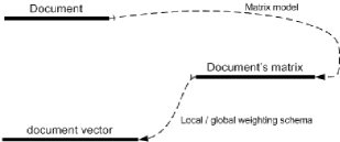
Refer to caption — Figure 1: Transition between matrix space and vector space.

As Figure 1 illustrates, MSM can be used as a transitional phase before producing the document vector. Given a tem $H\in\mathbb{R}^{m\times n}$ of a document $D$ , we can construct its vector space representation that is based on an arbitrary combination of local and/or global weighting scheme. As elements $h_{ij}$ of $H$ are based only on term frequency, the vector space representation of any document vector $a\in\mathbb{R}^{m}$ in the tdm can be written as $a=GHp$ , where $G\in\mathbb{R}^{m\times m}$ and $p\in\mathbb{R}^{n}$ . Matrix G is a diagonal matrix with nonzero diagonal elements accounting for the global weighting scheme. Column vector $p$ corresponds to the local weighting scheme applied on document $D$ . For example, $G=I$ corresponds to the application of no global weighting scheme, while $p=e$ corresponds to “term frequency” local weighting. Hereafter, we will assume that transition from matrix space to vector space is done by applying $G=I$ and $p=e$ to the tem. However, our results can be generalized to include more complex weighting schemes.

In the following section, we study MSM based upon document representation using tsm’s. For simplicity, we define a “sentence” to be text delimited between two consecutive periods (“.”). We do not address here the interesting issues involved in sentence identification (e.g. see [8, 17].)

2.1 Text analysis based on sentences.

Let $A$ denote a tdm of rank $r$ and let its SVD be

A=U\Sigma V^{\top}=\sum_{i=1}^{r}\sigma_{i}u_{i}v_{i}^{\top},

(2.1)

where the rightmost expression is the dyadic decomposition and, as usual, the singular values are arranged in non-increasing order. We also write ${\rm best}_{k}(A)$ for the best rank- $k$ approximation of $A$ (we assume here that $\sigma_{k}>\sigma_{k+1}$ ):

{\rm best}_{k}(A)=\sum_{i=1}^{k}\sigma_{i}u_{i}v_{i}^{\top}

(2.2)

Note also that

\begin{array}[]{rcl}a_{j}&=&\left(\sum_{i=1}^{r}\sigma_{i}u_{i}v_{i}^{\top}\right)_{j}=\sum_{i=1}^{r}\sigma_{i}u_{i}v_{ij}\end{array}

(2.3)

and similarly for the $j$ -th column of ${\rm best}_{k}(A)$ :

{\rm best}_{k}(A)e_{j}=\sum_{i=1}^{k}\sigma_{i}u_{i}v_{ij}

(2.4)

Having assumed that matrix $A$ is a tdm, the $j$ -th column of $A$ will correspond to the vector space representation of the $j$ -th document of the collection. So, we can write

a_{j}=\sum_{k=1}^{m}s_{k},

(2.5)

where $s_{k}$ , $k=1\dots m$ , is the vector space representation of the $k$ -th sentence of document $j$ of the collection and $m$ the total number of sentences of the $j$ -th document. We can now construct the tsm of document $j$ of our collection according to the following definition:

Definition 2.1

Let document $D$ contain $m$ sentences and $d$ be its vector space representation. The term-by-sentence matrix of document $D$ is the matrix

S_{D}=\left[s_{1},s_{2},\dots,s_{m}\right],

(2.6)

where $s_{k}$ refers to the vector space representation of the $k$ -th sentence of $D$ .

Using the above notation, Equation 2.5 can be written as

a_{j}=Ae_{j}=S_{D}e^{(m)}.

(2.7)

We also introduce the notion of the “term-by-sentence matrix for a matrix collection”. For example, if we have two documents $D_{1},D_{2}$ , their tsm’s are $S_{D_{1}}$ and $S_{D_{2}}$ , and the usual tdm from the VSM is the matrix of two columns $A=[a_{1},a_{2}]$ , then the tsm for the collection is the matrix $S_{C}=[\widehat{S}_{D_{1}},\widehat{S}_{D_{2}}]$ , where $\widehat{S}_{D_{j}}$ is an embedding of the original $S_{D_{j}}$ into a matrix with as many rows (terms) as $A$ . In other words, we augment each one of the tsm’s $S_{D_{j}}$ with zero rows corresponding to those terms in the collection’s vocabulary but not present in $D_{j}$ . In general, we have the following:

Definition 2.2

Let $C$ be a collection of $k$ documents $D_{1},\ D_{2},\ \dots\ D_{k}$ , where the $i$ -th document consists of $m_{i}$ sentences. The term-by-sentence matrix of the collection $C$ is the matrix $S_{C}$ :

\begin{array}[]{rcl}S_{C}&=&\left[\widehat{S}_{D_{1}},\widehat{S}_{D_{2}},\dots\,\widehat{S}_{D_{k}}\right]\\ \end{array}

(2.8)

where $\widehat{S}_{D_{j}}$ is an embedding of the original $S_{D_{j}}$ into a zero matrix with as many rows as the tdm of the VSM representation for $C$ .

The MSM provides a more general framework for IR [14, 19]. Our objective, here, was to investigate the performance of such a scheme and evaluate it relative to LSI and VSM. As we show, in specific cases the method can achieve results similar to LSI with respect to accuracy measures such as precision and recall, while keeping the computational costs to the levels of simple VSM.

The rationale of our method is that by projecting sentence vectors of tsm’s onto the subspace spanned by the singular vectors corresponding to the $k$ largest singular values for some small value of $k$ , permits us to eliminate polysemy and synonymy phenomena within the document. This is accomplished by the rank reduction of tsm’s that SVD produces. It is obvious that, as these phenomena are eliminated locally in every document it will be difficult to improve on LSI.

However, when the method is applied to collections with documents whose context is not semantically specific but multi-topic (e.g. documents from web pages with news) or to collections with large percentage of different terms per document, we provide experimental evidence that its performance surpasses classic vector space and comes close to LSI’s performance. The objective is, when a document that refers to $k$ semantically well-separated topics is given as input, for the projection to identify the principal directions of these topics. Then, by using the projected sentence vectors (instead of the original ones) we can transition to the vector space (from the MSM that uses tsm) by constructing approximations to the vectors of the VSM tdm according to some weighting scheme. We would thus be referring to this tdm with approximated columns as “pseudo-tdm”. In particular, the $j$ -th column of matrix $A$ is not computed according to Equation 2.7 but as follows: Let $D_{j}$ the $j$ -th document, $S$ the corresponding tsm, $r$ its rank and $t$ the number of columns (sentences) of in $D_{j}$ . Then

\ \ S=\sum_{i=1}^{r}\sigma_{i}u_{i}v_{i}^{\top}\ \textrm{and}\ {\rm best}_{k^{\prime}}(S)=\sum_{i=1}^{k^{\prime}}\sigma_{i}u_{i}v_{i}^{\top},

(2.9)

where $k^{\prime}\leq r$ , $(\sigma_{i},u_{i},v_{i})$ are singular triplets of $S$ with the $\sigma_{i}$ ’s arranged in decreasing order, and $\sigma_{k^{\prime}}>\sigma_{k^{\prime}+1}$ . Then column $a_{j}$ of the pseudo-tdm $A$ can be constructed as

a_{j}={\rm best}_{k^{\prime}}(S)e^{(t)}.

(2.10)

The steps for the sentence-oriented algorithm we are experimenting with are shown in Table 1.

Algorithm: Construct pseudo-tdm based on tsm

Input: Document collection

\{D_{1},...,D_{m}\}

Output: Pseudo-tdm

A

I. For each document

D_{j}

1. Prepare tsm

S_{D_{j}}

2. Select

k^{\prime}\leq{\rm rank}(S)

a_{j}={\rm best}_{k^{\prime}}(S)e^{(t)}

II. Assemble pseudo-tdm

A:=[a_{1},...,a_{m}]

Table 1: Construction of pseudo-tdm from document collection.

Query vectors $q$ are therefore compared to the columns of the pseudo-tdm. Cosine similarity can be computed using the following formula:

\begin{array}[]{rcl}\cos\ \theta_{j}&=&\frac{\left(Ae_{j}\right)^{\top}q}{\|Ae_{j}\|_{2}\|q\|_{2}}\\ &=&\frac{\left(\sum_{t=1}^{m}\sum_{i=1}^{k^{\prime}}\sigma_{i}u_{i}^{\top}v_{i,t}\right)^{\top}q}{\|Ae_{j}\|_{2}\|q\|_{2}}\end{array}

(2.11)

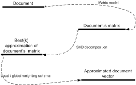
Figure 2 depicts schematically how MSM can be used to develop a new IR method. Transitional representation of a document in the matrix space permits the application of matrix transformations (in our case, approximation via SVD) before producing the vector that will represent the document in the tdm. Each approximated document vector is “assembled” from structures that are local to the document (substructures).

It is worth noting that in the algorithm presented in Table 1, each $k^{\prime}$ is selected to be $k^{\prime}\leq r$ , where $r$ is the rank of the particular tsm. Therefore, if we choose $k^{\prime}=r$ , the resulting vector becomes identical to the one obtained in the tdm of the classical VSM (before any weighting); furthermore, there is no need to perform an SVD of the tsm. Therefore, if this choice is made for every document, the whole pseudo-tdm reverts to the usual tdm, highlighting that MSM is a generalization of VSM.

2.2 Computational costs.

As with LSI, the method also relies on the (partial) SVD. The difference with LSI is that there are multiple SVD’s, one per tsm for each document. Note that the tsm’s can differ widely in size. Furthermore, the number of rows of each tsm will typically be much smaller than the full tdm since the number of terms in each sentence is expected to be much smaller than the total number of terms in the collection. More importantly, even though the approximate term-document vector resulting from this process for each document might be far less sparse than the term-document vector corresponding to the original tdm, many zeros will be introduced at the embedding phase, to take into account terms that are present in other documents but not this one. It is also worth noting, though we leave it for future study, that the SVD’s are independent for each document and hence can be processed in a distributed manner. It can happen, of course, that the number of sentences in each document can be large, even larger than the number of documents in the entire collection. To address this, we can make use of the flexibility of the proposed methodology, and adjust our analysis at any level of the document’s hierarchy that is convenient (sentences, paragraphs, sections, …). This is work in progress and we plan to report on it in the future. Table 2 illustrates indicative sizes for the tsm’s resulting from the MEDLINE datasets. These tsm’s appear to be small enough compared to the tdm and therefore the application of our method to them results on computational costs very close to that of VSM. We finally note that another advantage of this approach is that as the approximation is performed locally for each document, the method does not entail significant costs when performing document updates. In particular, the update of the pseudo-tdm using a new document will only cause a non-trivial change on existing document vectors if terms that already existed in these documents but were not accounted for till then, e.g. because of low global frequency. In that case, we would need to update, in some way, the SVD of the tsm of each affected document.

MED	terms	sentences	total	total
#	per doc.	per doc.	terms	docs.
1	45 (0.81%)	6 (0.58%)	5526	1033
2	90 (1.62%)	13 (0.62%)	5526	2066
3	135 (2.44%)	19 (0.61%)	5526	3099
4	180 (3.25%)	24 (0.58%)	5526	4132
5	225 (4.07%)	28 (0.54%)	5526	5165
6	270 (4.88%)	34 (0.55%)	5526	6198
7	315 (5.70%)	40 (0.55%)	5526	7231
8	360 (6.51%)	47 (0.57%)	5526	8264
9	405 (7.32%)	52 (0.56%)	5526	9297
10	450 (8.14%)	58 (0.56%)	5526	10330

Table 2: Example sizes for tsm’s (average number of terms and sentences per document for the datasets we used).

3 Analysis

To shed further light into the nature of the matrix resulting from tsm’s, in this section, we study the behavior of the singular values of a collection’s pseudo-tdm that has been constructed using this approach. We show that pseudo-tdm’s preserve the so-called low-rank-plus shift property of tdm’s([22]). Note that this property can be put to practical use to enhance the effectiveness of update algorithms ([27]). Even though we do not study such update schemes here, it is useful to know that they could be applied on pseudo-tdm’s.

Definition 3.1 (Low rank plus shift structure)

A matrix $A\in{\mathbb{R}}^{m\times n}$ is said to have “low rank plus shift” structure if it satisfies:

\frac{A^{\top}A}{m}\approx CWC^{\top}+\sigma^{2}I

(3.12)

where $C\in{\mathbb{R}}^{n\times k}$ and matrix $W\in{\mathbb{R}}^{k\times k}$ is a symmetric positive definite matrix.

When $A$ represents a collection’s tdm, $C\in{\mathbb{R}}^{n\times k}$ is the matrix whose columns represent latent concepts of the collection. The use of the terminology “low rank plus shift” comes from the fact that in IR applications, $k\ll\min\{m,n\}$ . The singular values of such matrices have the following distribution: The first few singular values are large but decrease rapidly and then the curve becomes flat but not necessarily zero. In order to determine if a matrix satisfies this property, we follow the analysis of Zha and Zhang ([27]) and investigate the following matrix approximation problem: Given a rectangular matrix, what is the closest matrix that has the low rank plus shift property. We can then define a matrix set for a given $k>0$ ,

	$\displaystyle J_{k}=\{B\in{\mathbb{R}}^{m\times n}\ \|\ \sigma_{1}(B)\geq\ldots\geq\sigma_{\min\{m,n\}}(B),$
	$\displaystyle\sigma_{k+1}(B)=\cdots=\sigma_{\min\{m,n\}}(B)\}$		(3.13)

Using this notation, the matrix approximation problem is reduced to finding the distance between a general matrix $A$ and the set $J_{k}$ . The next theorem provides as such a solution.

Theorem 3.1 (Zha and Zhang [22])

Let the SVD of $A$ be $A=U\Sigma V^{\top}$ , $\Sigma={\rm diag}[\sigma_{1},\ldots,\sigma_{\min\{m,n\}}]$ and $U,\ V$ orthogonal. Then for $k\leq\min\{m,n\}$ we have:

\displaystyle\arg\ \min_{J\in J_{k}}\|A-J\|_{p}=U_{k}\Sigma_{k}V_{k}^{\top}+\tau_{p}U_{^{\bot}}(V_{k}^{\bot})^{\top},

where $\Sigma_{k}={\rm diag}(\sigma_{1},\ldots,\sigma_{k}),U=[U_{k},U_{k}^{\bot}]$ , $V=[V_{k},V_{k}^{\bot}]$ and $p$ refers to either the Frobenius ( $p=F$ ) or the spectral ( $p=2$ ) norm. Furthermore,

\displaystyle\tau_{F}=\sum_{i=k+1}^{\min\{m,n\}}\frac{\sigma_{i}}{(\min\{m,n\}-k)}

and

\displaystyle\tau_{2}=\frac{\sigma_{k+1}+\sigma_{\min\{m,n\}}}{2}

Using the above theorem, we can examine experimentally how close is a given tdm to the set of matrices with the “low rank plus shift” structure. For our experimental analysis, we used the MEDLINE dataset that contains relatively small documents and one topic per document. We also constructed artificial, additional datasets based on MEDLINE, so as to test the performance of our method when applied to multi-topic documents. The documents of these datasets (MED_1, MED_2, …, MED_10) consist of joint documents of original MEDLINE. Documents of MED_i dataset, contain $i$ MEDLINE documents; MED_1 is identical to MEDLINE.

Table 3 shows the value of quantity $\frac{\|A-{\rm best}_{100}(A)\|_{F}}{\|A\|_{F}}$ for different tdm’s (pseudo-tdm and the usual VSM tdm). According to Theorem 3.1, the smaller this value is for a given matrix, the closer to low-rank-plus-shift structure the matrix is. The notation we use for the naming of the datasets is of the form NAME_i_j, where NAME is the dataset’s name, $i$ is the number of actual semantic topics per collection’s document and $j$ is the number of singular triplets of the term by sentences matrix that were used for the construction of approximated document vectors.

Dataset	VSM tdm	pseudo-tdm
MED_1_1	$0.6738$	$0.6655$
MED_2_1	$0.5973$	$0.5807$
MED_3_1	$0.5232$	$0.5030$
MED_4_1	$0.4601$	$0.4379$
MED_5_1	$0.4015$	$0.3746$
MED_6_1	$0.3462$	$0.3172$
MED_7_1	$0.2852$	$0.2534$
MED_8_1	$0.2282$	$0.1982$
MED_9_1	$0.1644$	$0.1411$
MED_10_1	$0.0829$	$0.0660$

Table 3: Value of

\frac{\|A-{\rm best}_{100}(A)\|_{F}}{\|A\|_{F}}

for a tdm constructed using VSM and our method (pseudo-tdm).

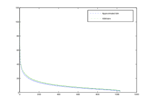
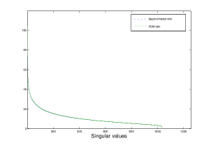
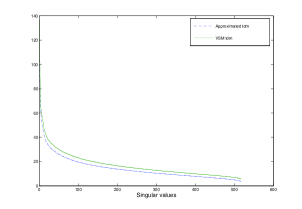
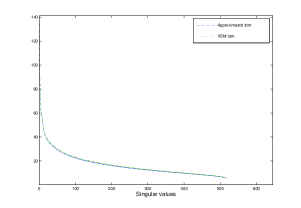
As depicted on Table 3, the pseudo-tdm’s appears to be closer to the “low rank plus shift” structure than the VSM tdm’s. Furthermore, the distance becomes even smaller for multi-topic collections. Figure 3 depicts singular value distributions for classic and approximated tdm’s of datasets ${\rm MED}\_1$ and ${\rm MED}\_2$ using $k^{\prime}=1,5$ singular triplets to approximate the tsm’s. We note that the singular values of pseudo-tdm’s are bounded by the corresponding singular values of VSM tdm’s. We next prove that this indeed holds.

3.1 Some spectral properties of pseudo-tdm’s.

In the sequel, when we compare the singular values of two matrices with the same number of rows but different number of columns we will count the singular values according to the number of rows. We first state three simple results.

Lemma 3.1

Let $A\in{\mathbb{R}}^{m\times n}$ . Let V be orthonormal. Then

\sigma_{i}\left(AV^{\top}\right)=\sigma_{i}\left(A\right),i=1,\ldots,m.

(3.14)

Lemma 3.2

Let $A=[A_{1},A_{2}]$ . Then

\sigma_{i}\left(A_{1}\right)\leq\sigma_{i}\left(A\right),i=1,\ldots,m.

(3.15)

Lemma 3.3

Let $A,B\in\mathbb{R}^{m\times n}$ and $q=\min\{m,n\}$ . Then

\displaystyle\sigma_{i}\left(AB^{\top}\right)\leq\sigma_{i}(A)\sigma_{1}(B),i=1,\ldots,q.

We next consider the tsm of a collection with two documents. The following theorem comes as a generalization of a similar result of Zha and Simon [22, Theorem 3.3].

Theorem 3.2

Let $A\in{\mathbb{R}}^{m\times n}$ and write $A=[A_{1},A_{2}]$ . Then for any $k_{1}$ , $k_{2}$ , we have

\displaystyle\sigma_{i}\left([{\rm best}_{k_{1}}\left(A_{1}\right),{\rm best}_{k_{2}}\left(A_{2}\right)]\right)\leq\sigma_{i}\left([A_{1},A_{2}]\right).

Proof.

In the sequel, we remind that the SVD of a matrix $A$ can be written as

\displaystyle A=[P_{k},P_{k}^{\bot}]{\rm diag}(\Sigma_{k},\Sigma_{k}^{\bot})([Q_{k},Q_{k}^{\bot}])^{\top},

where $P_{k},\Sigma_{k},Q_{k}$ consists of the $k$ leading left and write singular triplets and $P_{k}^{\bot},\Sigma_{k}^{\bot},Q_{k}^{\bot}$ the remaining ones. Clearly, $P_{k}^{\top}P_{k}^{\bot}$ and $Q_{k}^{\top}Q_{k}^{\bot}$ are 0 matrices. Then, for $i=1,\ldots,m$ , $\sigma_{i}([A_{1},A_{2}])=$

\displaystyle\begin{array}[]{lcl}&=&\sigma_{i}\left([[P_{k_{1}},P_{k_{1}}^{\bot}]{\rm diag}(\Sigma_{k_{1}},\ \Sigma_{k_{1}}^{\bot}),A_{2}]\right)\\ &=&\sigma_{i}\left([P_{k_{1}}\Sigma_{k_{1}},A_{2},P_{k_{1}}^{\bot}\Sigma_{k_{1}}^{\bot}]\right)\\ &=&\sigma_{i}\left([P_{k_{1}}\Sigma_{k_{1}}Q_{k_{1}}^{\bot},A_{2},P_{k_{1}}^{\bot}\Sigma_{k_{1}}^{\bot}]\right)({\rm by\ Lemma\ \ref{lem:singular_orthonormal}})\\ &=&\sigma_{i}\left([{\rm best}_{k_{1}}(A_{1}),[P_{k_{2}},P_{k_{2}}^{\bot}]{\rm diag}(\Sigma_{k_{2}},\Sigma_{k_{2}}^{\bot}),P_{k_{1}}^{\bot}\Sigma_{k_{1}}^{\bot}]\right)\\ &=&\sigma_{i}\left([{\rm best}_{k_{1}}(A_{1}),P_{k_{2}}\Sigma_{k_{2}},P_{k_{2}}^{\bot}\Sigma_{k_{2}}^{\bot},P_{k_{1}}^{\bot}\Sigma_{k_{1}}^{\bot}]\right)\\ &=&\sigma_{i}\left([{\rm best}_{k_{1}}(A_{1}),P_{k_{2}}\Sigma_{k_{2}}Q_{k_{2}}^{\bot},P_{k_{2}}^{\bot}\Sigma_{k_{2}}^{\bot},P_{k_{1}}^{\bot}\Sigma_{k_{1}}^{\bot}]\right)\\ &=&\sigma_{i}\left([{\rm best}_{k_{1}}(A_{1}),{\rm best}_{k_{2}}(A_{2}),P_{k_{2}}^{\bot}\Sigma_{k_{2}}^{\bot},P_{k_{1}}^{\bot}\Sigma_{k_{1}}^{\bot}]\right).\end{array}

Noticing that $[{\rm best}_{k_{1}}(A_{1}),\ {\rm best}_{k_{2}}(A_{2})]$ is a submatrix of $[{\rm best}_{k_{1}}(A_{1}),{\rm best}_{k_{2}}(A_{2}),P_{k_{2}}^{\bot}\Sigma_{k_{2}}^{\bot},P_{k_{1}}^{\bot}\Sigma_{k_{1}}^{\bot}]$ we obtain the result by invoking Lemma 3.2.

Using Theorem 3.2, we can prove the following result for the approximate tdm constructed by our method.

Theorem 3.3

Let $A\in\mathbb{R}^{m\times n}$ and write $A=[A_{1},A_{2}]$ where $A_{1}\in\mathbb{R}^{m\times n_{1}}$ and $A_{2}\in\mathbb{R}^{m\times n_{2}}$ . Then for any $k_{1}$ , $k_{2}$ , we have

	$\displaystyle\ \ \sigma_{i}\left([{\rm best}_{k_{1}}\left(A_{1}\right)e^{(n_{1})},{\rm best}_{k_{2}}\left(A_{2}\right)e^{(n_{2})}]\right)$		(3.17)
	$\displaystyle\leq\ \ \ \ \ \ \ \sigma_{i}\left([A_{1}e^{(n_{1})},A_{2}e^{(n_{2})}]\right)$

Proof.

Let $\widehat{A}=[{\rm best}_{k_{1}}(A_{1}),{\rm best}_{k_{2}}(A_{2})]$ . Then we have:

	$\displaystyle[A_{1}e^{(n_{1})},A_{2}e^{(n_{2})}]$	$\displaystyle=$	$\displaystyle[A_{1},A_{2}]\left[\begin{array}[]{cc}e^{(n_{1})}&0\\ 0&e^{(n_{2})}\\ \end{array}\right]$		(3.20)
		$\displaystyle=$	$\displaystyle A\left[\begin{array}[]{cc}e^{(n_{1})}&0\\ 0&e^{(n_{2})}\\ \end{array}\right]$		(3.23)

and

\displaystyle[{\rm best}_{k_{1}}(A_{1})e^{(n_{1})},{\rm best}_{k_{2}}(A_{2})e^{(n_{2})}]

\displaystyle=

\displaystyle\widehat{A}\left[\begin{array}[]{cc}e^{(n_{1})}&0\\ 0&e^{(n_{2})}\\ \end{array}\right]

(3.26)

We now define

B^{\top}=\left[\begin{array}[]{cc}e^{(n_{1})}&0\\ 0&e^{(n_{2})}\\ \end{array}\right]

and by invoking Lemma 3.3, we have:

	$\displaystyle\sigma_{i}([A_{1}e^{(n_{1})},A_{2}e^{(n_{2})}])\leq\sigma_{i}(A)\sigma_{1}(B)$
	$\displaystyle\sigma_{i}([{\rm best}_{k_{1}}(A_{1})e^{(n_{1})},{\rm best}_{k_{2}}(A_{2})e^{(n_{2})}])\leq\sigma_{i}(\widehat{A})\sigma_{1}(B)$

As $\sigma_{i}(\widehat{A})\leq\sigma_{i}(A)$ (by Theorem 3.2) the result follows.

Theorem 3.3 is readily generalized to provide bounds for the singular values of matrices $A=[A_{1},A_{2},\dots A_{k}]$ that correspond to collection’s tem’s with $k$ documents.

Note that since every term of the pseudo-tdm vector that corresponds to the $j$ -th document is the result of a local operation on the document’s tsm, namely $a_{j}={\rm best}_{k^{\prime}}(S)e^{(t)}$ , the construction of each element of $a_{j}$ can be interpreted as the result of a weight factor based on local information applied on the corresponding term of $Se^{(t)}$ .

MED	VSM	New	LSI	LSI	New w.
#			$k=20$	$k=100$	LSI(20)
1	$0.0313$	0.0314	0.0284	0.0285	0.0279
2	$0.0754$	0.0728	0.0697	0.0815	0.0633
3	$0.0544$	0.052	0.0595	0.0503	0.0563
4	$0.0793$	0.0797	0.0866	0.0802	0.0919
5	$0.0809$	0.0795	0.0888	0.0842	0.094
6	$0.088$	0.0883	0.0949	0.0898	0.1027
7	$0.0866$	0.0904	0.0962	0.0897	0.092
8	$0.0862$	0.0928	0.0938	0.0867	0.1116
9	$0.1031$	0.1041	0.1057	0.105	0.0992
10	$0.1048$	0.1077	0.1015	0.1035	0.1016

Table 4: Mean precision for MEDLINE datasets. The pseudo-tdm vectors were computed with

k^{\prime}=5

singular triplets.

4 Experimental results

All experiments were conducted using MATLAB 6.5 running using Windows XP on a 2.4 GHz Pentium IV PC with 512 MB of RAM. In all cases we compute the necessary singular triplets by means of the MATLAB svds function that is based on implicitly restarted Arnoldi [15]. Our focus was query evaluation using Equation 2.11 on the pseudo-tdm constructed via the Algorithm of Table 1. We tested the new method using $k^{\prime}=1$ and $5$ tsm singular triplets to build the pseudo-tdm. We also used the new method in combination with LSI, that is applying LSI on the pseudo-tdm, to get an appreciation of the overall performance. These results were compared with simple VSM (term frequency local weighting) and LSI using the approximated tdm of rank $k=20,100$ . All experiments were conducted using Text to Matrix Generator (tmg), a recent MATLAB toolbox [26]. To this effect, we also enhanced TMG’s functionality to permit the creation of tsm’s and pseudo-tdm’s.
Tables 4 and 5 tabulate the mean precision of VSM, LSI (based on 20 and 100 singular triplets) and the new method for the different MEDLINE datasets. They also illustrate the performance of the method when it is combined with LSI (column “New w. LSI” of Tables 4, 5).

MED	VSM	New	LSI	LSI	New w.
#			$k=20$	$k=100$	LSI(20)
1	0.0313	0.0325	0.0284	0.0285	0.0283
2	0.0754	0.0657	0.0697	0.0815	0.0576
3	0.0544	0.0527	0.0595	0.0503	0.0534
4	0.0793	0.077	0.0866	0.0802	0.0779
5	0.0809	0.0792	0.0888	0.0842	0.0809
6	0.088	0.0816	0.0949	0.0898	0.0903
7	0.0866	0.0903	0.0962	0.0897	0.0948
8	0.0862	0.0867	0.0938	0.0867	0.103
9	0.1031	0.1008	0.1057	0.105	0.0949
10	0.1048	0.1006	0.1015	0.1035	0.1005

Table 5: Mean precision for MEDLINE datasets. The pseudo-tdm vectors were computed with

k^{\prime}=1

singular triplets.

Tables 6, 7 present the number of queries that each method answers with greater precision, compared to the precision of the other method’s answers. The new method appears to offer significant improvements over the performance of VSM, while in many cases the new methods performs better than LSI.

MED	VSM	New	LSI	LSI
#			$k=20$	$k=100$
1	2(7%)	9(30%)	9(30%)	7(23%)
2	3(10%)	8(27%)	9(30%)	9(30%)
3	4(13%)	3(10%)	14(47%)	8(27%)
4	4(13%)	7(23%)	15(50%)	4(13%)
5	4(13%)	6(20%)	13(43%)	5(17%)
6	3(10%)	7(23%)	11(37%)	7(23%)
7	4(13%)	9(30%)	13(43%)	2(7%)
8	3(10%)	5(17%)	14(47%)	7(23%)
9	2(67%)	7(23%)	9(30%)	10(33%)
10	6(20%)	9(30%)	13(43%)	1(3%)

Table 6: Number of queries that each method answers with greater precision for MEDLINE datasets. The pseudo-tdm vectors were computed with

k^{\prime}=5

singular triplets.

MED	VSM	New	LSI	LSI
#			$k=20$	$k=100$
1	1(3%)	15(50%)	7(23%)	6(20%)
2	4(7%)	8(27%)	9(30%)	9(30%)
3	3(10%)	7(23%)	14(47%)	6(20%)
4	4(13%)	6(20%)	14(47%)	5(17%)
5	4(13%)	6(20%)	14(47%)	5(17%)
6	4(13%)	9(30%)	8(27%)	7(23%)
7	5(17%)	8(27%)	11(37%)	4(13%)
8	3(10%)	7(23%)	13(43%)	5(17%)
9	1(3%)	8(27%)	8(27%)	11(37%)
10	7(23%)	8(27%)	12(40%)	3(10%)

Table 7: Number of queries that each method answers with greater precision, for MEDLINE datasets. The pseudo-tdm vectors were computed with

k^{\prime}=1

singular triplets.

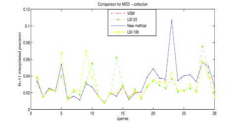
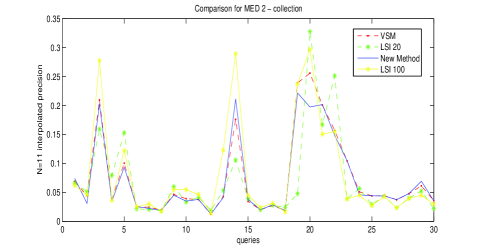
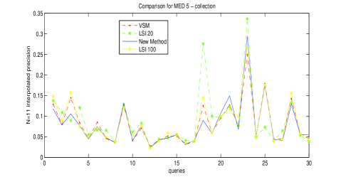
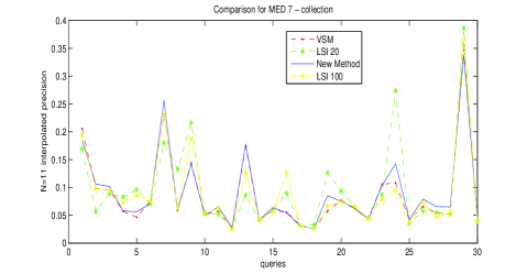
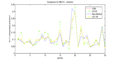
We also plot, in Figure 6, the $N=11$ -point interpolated average precision for the different queries of MEDLINE datasets. The interpolated precision is defined as:

\displaystyle p=\frac{1}{N}\sum_{i=0}^{N}\widehat{p}\left(\frac{i}{N-1}\right)

where:

\displaystyle\widehat{p}\left(x\right)=\max\{p_{i}\ \mid\ n_{i}\geq xr\ ,i=1:r\}

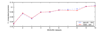
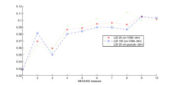
Figure 4 illustrates the performance of the new method (using 5 singular triplets to approximate the tsms) compared to VSM. Figure 5 provides experimental results for the new method viewed as an alternative weighting scheme. The new method and VSM have similar performance on datasets MED_1 to MED_5. However, for MED_6 to MED_10, the new method improves VSM. These results imply that the SVD approximation of tsm’s indeed captures the topic directions of multi-topic documents and thus improves the overall IR performance. Furthermore, LSI’s performance improves when based upon the pseudo-tdm.
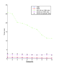
Finally, in order to gain an appreciation for the method’s cost, we present in Figure 7 the runtimes for performing a query on tdm’s that correspond to classical VSM, LSI with values of $k=20$ and 100, the new method, and finally the combination of LSI with the new method. In all experiments, times include the cost of performing the necessary partial SVD’s. Results indicate the new method has runtimes similar to VSM.

5 Conclusions

Our theoretical and experimental results suggest that, at the sentence level, matrix space models that have greater awareness of each document’s local structure and are able to capture additional semantic information for each document, can be successfully used to improve existing IR techniques. Our results provide significant evidence that further justify proposals such as those in [14, 19] towards the use of matrix based models and provide additional tools for IR in such frameworks. We are currently studying the effects of enabling additional levels of analysis (not only based on sentences) and adding overall greater flexibility in the algorithm, as well as the utilization of multilinear algebra techniques (cf. [16]) and the use of parallel processing.

Acknowledgments.

We thank the referees for their suggestions.

References

[1] D. Achlioptas and F. McSherry. Fast Computation of Low Rank Matrix Approximations. In Proc 33rd Annual ACM Symposium on Theory of Computing, pages 611–618, 2001.
[2] I. Antonellis, C. Bouras, and V. Poulopoulos. Personalized news categorization through scalable text classification. In Proc 8th Asia-Pasific Web Conf, pages 391–401, 2006.
[3] M. Berry. Large Scale Sparse Singular Value Computations. Int’l. J. Supercomputing Applications, 6:13–49, 1992.
[4] M. Berry, Z. Drmac, and E. Jessup. Matrices, vector spaces, and information retrieval. SIAM Review, 41:335–362, 1998.
[5] M.W. Berry and M. Brown. Understanding Search Engines. SIAM, Philadelphia, 1999.
[6] P. E. Bjørstad and O. Widlund. Iterative methods for the solution of elliptic problems on regions partitioned into substructures. SIAM J. Numer. Anal., 23(6):1097–1120, December 1986.
[7] K. Blom and A. Ruhe. A Krylov subspace method for Information Retrieval. SIAM J. Matrix Anal. Appl., 26:566–582, 2005.
[8] M. Castellanos. Hot-Miner: Discovering hot topics from dirty text. In M.W. Berry, editor, Survey of Text Mining: Clustering, Classification, and Retrieval, pages 123–157. Springer Verlag, 2003.
[9] V. Castelli, A. Thomasian, and C.-S. Li. CSVD: Clustering and singular value decomposition for approximate similarity search in high-dimensional spaces. IEEE Trans. Knowledge and Data Engin., 15(3):671–685, 2003.
[10] S. Deerwester, S. Dumais, G. Furnas, T. Landauer, and R. Harshman. Indexing by Latent Semantic Analysis. Journal of the American Society for Information Science, 41(6):391–407, 1990.
[11] P. Drineas, A. Frieze, R. Kannan, S. Vempala, and V. Vinay. Clustering large graphs via the singular value decomposition. Mach. Learn., 56(1-3):9–33, 2004.
[12] L. Elden. Numerical linear algebra in data mining. In Acta Numerica. Cambridge University Press, Cambridge, 2006 (to appear).
[13] H. Kargupta, W. Huang, K. Sivakumar, and E.L. Johnson. Distributed clustering using collective principal component analysis. Knowledge and Information Systems, 3(4):422–448, 2001.
[14] M.S. Kamel K.M. Hammouda. Efficient phrase-based document indexing for Web document clustering. IEEE Trans. Knowl. Data Eng., 16(10):1279–1296, Oct. 2004.
[15] R. Lehoucq, D.C. Sorensen, and C. Yang. Arpack User’s Guide: Solution of Large-Scale Eigenvalue Problems With Implicitly Restarted Arnoldi Methods. SIAM, Philadelphia, 1998.
[16] N. Liu, B. Zhang, J. Yan, Z. Chen, W. Liu, F. Bai, and L. Chien. Text representation: From vector to tensor. In Proc. 5th IEEE Int’l. Conf. Data Mining (ICDM’04), pages 725–728. IEEE, 2005.
[17] D.D. Palmer, M.A. Hearst. Adaptive sentence boundary disambiguation. In Proc. 4th Conf. on Applied Natural Language Processing, pp 78-83, San Francisco, CA, USA, 1994. Morgan Kaufmann Publishers Inc.
[18] C.H. Papadimitriou, P. Raghavan, H. Tamaki, and S. Vempala. Latent Semantic Indexing: A Probabilistic analysis. J. Comput. Syst. Sci., 61(2):217–235, 2000.
[19] T. Roelleke, T. Tsikrika, and G. Kazai. A general matrix framework for modelling information retrieval. J. Information Processing & Management, 42:4–30, 2006.
[20] G. Salton, A. Wong, and C. S. Yang. A vector space model for automatic indexing. Comm. ACM, 18(11):613–620, 1975.
[21] J. D. Schlesinger, J. M. Conroy, M. E. Okurowski, and D. P. O’Leary. Machine and human performance for single- and multi-document summarization. IEEE Intelligent Systems (special issue on Natural Language Processing), 18:46–54, 2003.
[22] H. Simon and H. Zha. On updating problems in latent semantic indexing. SIAM J. Sci. Comput., 21:782–791, 1999.
[23] H.D. Simon and H. Zha. Low-rank matrix approximation using the Lanczos bidiagonalization process with applications. SIAM J. Sci. Comp., 21(6):2257–2274, 2000.
[24] H. Wu and D. Gunopulos. Evaluating the utility of statistical phrases and latent semantic indexing for text classification. In Proc. 2002 IEEE Int’l. Conf. Data Mining (ICDM 2002), pages 713–716. IEEE Computer Society, 2002.
[25] D. Zeimpekis and E. Gallopoulos. CLSI: A flexible approximation scheme from clustered term-document matrices. In H. Kargupta et al., editor, Proc. Fifth SIAM Int’l Conf. Data Mining (Newport Beach), pages 631–635, Philadelphia, April 2005. SIAM. For an extended version, see Tech. Report HPCLAB-SCG 2/10-04.
[26] D. Zeimpekis and E. Gallopoulos. TMG: A MATLAB Toolbox for generating term-document matrices from text collections. In J. Kogan, C. Nicholas, and M. Teboulle, editors, Grouping Multidimensional Data: Recent Advances in Clustering, pages 187–210. Springer, 2006.
[27] H. Zha and Z. Zhang. Matrices with low-rank-plus-shift structure: Partial SVD and latent semantic indexing. SIAM J. Matrix Anal. Appl., 21(2):522–536, 2000.

Exploring term-document matrices from matrix models in text mining††thanks: Work conducted in the context of and supported in part by a University of Patras KARATHEODORI grant.

Abstract

1 Introduction

2 Matrix space models for IR

2.1 Text analysis based on sentences.

Definition 2.1

Definition 2.2

2.2 Computational costs.

3 Analysis

Definition 3.1 (Low rank plus shift structure)

Theorem 3.1 (Zha and Zhang [22])

3.1 Some spectral properties of pseudo-tdm’s.

Lemma 3.1

Lemma 3.2

Lemma 3.3

Theorem 3.2

Theorem 3.3

4 Experimental results

5 Conclusions

Acknowledgments.

References

Exploring term-document matrices from matrix models in text mining^†^†thanks: Work conducted in the context of and supported in part by a University of Patras KARATHEODORI grant.