Geographic Gossip: Efficient Aggregation for Sensor Networks

Abstract

Gossip algorithms for aggregation have recently received significant attention for sensor network applications because of their simplicity and robustness in noisy and uncertain environments. However, gossip algorithms can waste significant energy by essentially passing around redundant information multiple times. For realistic sensor network model topologies like grids and random geometric graphs, the inefficiency of gossip schemes is caused by slow mixing times of random walks on those graphs. We propose and analyze an alternative gossiping scheme that exploits geographic information. By utilizing a simple resampling method, we can demonstrate substantial gains over previously proposed gossip protocols. In particular, for random geometric graphs, our algorithm computes the true average to accuracy $1/n^{a}$ using $O(n^{1.5}\sqrt{\log n})$ radio transmissions, which reduces the energy consumption by a $\sqrt{\frac{n}{\log n}}$ factor over standard gossip algorithms.

Categories and Subject Descriptors: F.2.2, G.3

General Terms: algorithms

Keywords: gossip algorithms, random geometric graphs, sensor networks, distributed consensus, distributed aggregation

1 Introduction

Consider a network of $n$ sensors, in which each node collects a measurement in some modality of interest (e.g., temperature, light, humidity etc.). It is frequently of interest to solve the averaging problem: namely, to develop a distributed and fault-tolerant algorithm by which all nodes can compute the average of all $n$ sensor measurements. Gossip algorithms solve the averaging problem by having each node randomly pick one of their one-hop neighbors and exchange their current values. The pair of nodes compute the pairwise average, which then becomes the new value for both nodes. By iterating this pairwise averaging process, it is easy to show that all the nodes converge to the global average in a completely distributed manner. Although fairly simple, the distributed averaging problem and related consensus problems can be viewed as building blocks for solving more complex problems [19, 21], including computing general linear functions as well as optimization of non-linear functions in sensor networks.

The key issue is how many iterations it takes for such gossip algorithm to converge to a sufficiently accurate estimate. Variations of this problem have received significant attention in recent work [11, 12, 4, 5]. The convergence speed of a nearest-neighbor gossip algorithm, known as the averaging time, turns out to be closely linked to the mixing time of the Markov chain defined by a weighted random walk on the graph. Boyd et al. [4] showed how to optimize the neighbor selection probabilities for each node so to find the fastest-mixing Markov chain on the graph. For certain types of graphs, including complete graphs, expander graphs and peer-to-peer networks, such Markov chains are rapidly mixing, so that gossip algorithms converge very quickly.

Unfortunately, for the graphs corresponding to typical wireless sensor networks, even an optimized gossip algorithm can result in very high energy consumption. For example, a common model for an wireless sensor network is a random geometric graph [17], in which all nodes communicate with neighbors within a radius $r$. With the transmission radius scaling in the standard way as $r(n)=\Theta(\sqrt{\frac{\log n}{n}})$, even an optimized gossip algorithm requires $\Theta(n^{2})$ transmissions (see section 2.3), which is of the same order as the energy required for every node to flood its value to all other nodes. This problem is noted in [4]: “In a wireless sensor network, Theorem 6 suggests that for a small radius of transmission, even the fastest averaging algorithm converges slowly”, and it seems to be fundamental for gossip algorithms on these graphs. Intuitively, the nodes in a standard gossip protocol are essentially “blind”, and they repeatedly compute pairwise averages with their one-hop neighbors. Information only diffuses slowly throughout the network, roughly moving distance $\sqrt{k}$ in $k$ iterations (as a random walk).

Accordingly, the goal of this paper is to develop and analyze alternative —and ultimately more efficient— methods for solving distributed averaging problems in wireless networks. We leverage the fact that sensors nodes typically know their locations, and can therefore use this knowledge to perform geographic routing. Localization is a well studied problem (e.g., [20, 13]), since geographic knowledge is required in numerous applications. With this perspective in mind, we propose an algorithm that, like a standard gossiping protocol, is completely randomized, distributed and robust, but requires substantially less communication by exploiting geographic information. The idea is that instead of exchanging information with one-hop neighbors, geographic routing can be used to gossip with random nodes who are far away in the network. We show that the extra cost of multi-hop routing is compensated by the rapid diffusion of information.

The remainder of this paper is organized as follows. In Section 2, we provide a precise statement of the distributed averaging problem, describe our algorithm, and state our main results on its performance. Section 3 contains proofs of these technical results. In Section 4, we experimentally evaluate the performance of our algorithm.

2 Proposed Algorithm and Main Results

2.1 Problem statement

2.1.1 Graph model

Following previous work [8, 4], we model our wireless sensor network as a random geometric graph [17]. In this model, denoted $G(n,r)$, the $n$ sensor locations are chosen uniformly and independently in the unit square, and each pair of nodes is connected if their Euclidean distance is smaller than some transmission radius $r$. (As discussed in Section 5, our results have natural analogs for lattices, and other graph structures that are reasonable models of wireless networks). It is well known [17, 8, 7] that in order to have good connectivity and minimize interference, the transmission radius $r(n)$ has to scale like $\Theta(\sqrt{\frac{\log n}{n}})$. For our analysis, we assume that communication within this transmission radius always succeeds. Note however that the proposed algorithm is very robust to communication and node failures.

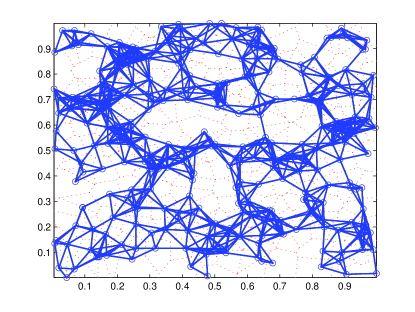
Figure 1: Illustration of a random geometric graph. The solid lines represent graph connectivity, and the dotted lines show the Voronoi regions associated with each node.

2.1.2 Time model

We use the asynchronous time model [4], which is well-matched to the distributed nature of sensor networks. More precisely, it is assumed that each sensor node has a clock which ticks independently as a rate $\lambda$ Poisson process. Consequently, the inter-tick times are exponentially distributed, and independent across nodes and across time. This set-up is equivalent to a single clock ticking according to a rate $n\lambda$ Poisson process at times $Z_{k}$. On average, there are approximately $n$ clock ticks per unit of absolute time (an exact analysis can be found in [4]) but we will always be measuring time in number of ticks of this (virtual) global clock. Time is discretized, and the interval $[Z_{k},Z_{k+1})$ corresponds to the $k$th timeslot. We can adjust time units relative to the communication time so that only one packet exists in the network at each time slot with high probability.

2.1.3 Distributed averaging

At time slot $k=0,1,2\ldots$, each node $i=1,\ldots,n$ has an estimate $x_{i}(k)$ of the global average, and we use $x(k)$ to denote the $n$-vector of these estimates. The ultimate goal is to drive the estimate $x(k)$ to the average $\bar{x}_{\operatorname{ave}}\vec{1}$, where $\bar{x}_{\operatorname{ave}}:\,=\frac{1}{n}\sum_{i=1}^{n}x_{i}(0)$, using the minimal amount of communication. For the algorithms of interest to us, the quantity $x(k)$ for $k>0$ is a random vector, since the algorithms are randomized in their behavior. Accordingly, we measure the convergence of $x(k)$ to $x(0)$ in the following sense [12, 4] (essentially convergence in probability):

Definition 1

Given $\epsilon>0$, the $\epsilon$-averaging time is the earliest time at which the vector $x(k)$ is $\epsilon$ close to the normalized true average with probability greater than $1-\epsilon$:

$$T_{ave}(n,\epsilon)=\sup_{x(0)}\inf\left\{k:\mathbb{P}\left(\frac{\|x(k)-x_{ave}\vec{1}\|}{\|x(0)\|}\geq\epsilon\right)\leq\epsilon\right\}~{}.$$ (1)

where $\|\cdot\|_{2}$ denotes the $\ell_{2}$ norm.

Let $R(k)$ represent the number of one-hop radio transmissions required for a given node to communicate with some other node at time click $k$. In a standard gossip protocol, the quantity $R(k)\equiv R$ is simply a constant, whereas for our protocol, $R(k)$ will be a random variable (with identical distribution for each node). The total communication cost is measured by the random variable

$$\mathcal{C}(n,\epsilon)=\sum_{k=1}^{T_{ave}(n,\epsilon)}R(k)~{}.$$ (2)

In this paper, we first analyze the expected communication cost, denoted by $\mathcal{E}(n,\epsilon)$, which is given by

$$\mathcal{E}(n,\epsilon)=E[R(k)]T_{ave}(n,\epsilon)~{}.$$ (3)

In addition, we provide a upper bound on the communication cost, denoted by $\mathcal{D}(n,\epsilon)$, such that

$$\mathbb{P}\Big{\{}\mathcal{C}(n,\epsilon)\geq\mathcal{D}(n,\epsilon)\Big{\}}\leq\frac{\epsilon}{2}~{}.$$ (4)

2.2 Proposed Algorithm

The proposed algorithm combines gossip with geographic routing. The key assumption is that each node knows its geographic location. With that knowledge, every node can also learn the locations of its one-hop neighbors by having just one transmission per node.

Suppose the $j$-th clock to tick belongs to node $s$. Let $l(s)$ denote the location of node $s$. Node $s$ activates and does the following:

1. Node $s$ chooses a point uniformly in the unit square. Call this the target $t$. Node $s$ forms the tuple $m_{s}=(x_{s}(j),l(s),t)$.

2. Node $s$ sends $m_{s}$ to its one-hop neighbor closest to $t$, if any exists. If node $r$ receives a packet $m_{s}$, it sends $m_{s}$ to its one-hop neighbor closest $t$. Greedy geographic routing terminates when a node receives the packet and has no one-hop neighbors with distance smaller to the random target that its own. Let $v$ be the node closest to $t$.

3. Node $v$ makes an independent randomized decision to accept $m_{s}$. If the packet is accepted, $v$ computes its new value $x_{v}(j+1)=(x_{v}(j)+x_{s}(j))/2$ and a message $m_{v}=(x_{v}(j),l(v),l(s))$ is sent back to $s$ via greedy geographic routing. Node $s$ computes $x_{s}(j+1)=(x_{v}(j)+x_{s}(j))/2$, and the round ends.

4. If the packet is rejected, $v$ chooses a new point $t^{\prime}$ uniformly in the plane and repeats steps 2–3 with message $m^{\prime}_{s}=(x_{s}(j),l(s),t^{\prime})$.

We will refer to this procedure as a gossip round. Our analysis of this randomized algorithm, given in Section 3, consists of the following steps. First, we prove that when $r(n)=\Theta(\sqrt{\frac{\log n}{n}})$, greedy routing always reaches the closest node $v$ to the random target in $O(\sqrt{\frac{n}{\log n}})$ radio transmissions. Note that in practice more sophisticated geographic routing algorithms (e.g., [10]) can be used to ensure that the packet approaches the random target when there are “holes” in the node density. However, greedy geographic routing is good enough for our model and other choices for routing algorithms will not affect our results.

Our randomized procedure induces a probability distribution over the chosen sensor $v$ (i.e., the one closest to the randomly chosen target). If this distribution were uniform, then it follows immediately that the averaging time $T_{ave}(n,\epsilon)$ is $\mathcal{O}(n\log\epsilon^{-1})$. In actuality, the probability of choosing sensor $v$ is equal to $a_{v}$, the area of its associated Voronoi region. The distribution of Voronoi regions is not very uniform, so in order to bound the averaging time $T_{ave}(n,\epsilon)$, we apply rejection sampling in order to temper the distribution. In particular, we apply the following rejection sampling scheme, due to Bash et al. [2]. Let $\vec{a}$ be an $n$-vector of areas of the sensors’ Voronoi regions. We set a threshold $\tau$ on the cell areas. Sensors with cell area smaller than $\tau$ always accept a query, and sensors with cell areas larger than $\tau$ reject the query with a certain probability. The rejection sampling method protects against oversampling and limits the number of undersampled sensors, and allows us to prove that $T_{ave}(n,\epsilon)=\mathcal{O}(n\log\epsilon^{-1})$, even for this perturbed distribution.

Of course, the rejection sampling scheme requires some random number $Q$ of queries before a sensor accepts. In terms of the number of queries, the total number of radio transmissions for the $k$th gossip round is

$$R(k)=O\left(Q\sqrt{\frac{n}{\log n}}\right).$$ (5)

Therefore if $T_{ave}$ gossip rounds take place overall, the expected of radio transmissions will be

$$\mathcal{E}(n,\epsilon)=\mathbb{E}[Q]\mathcal{O}\left(\sqrt{\frac{n}{\log n}}\right)T_{ave}(n,\epsilon)~{}.$$ (6)

Accordingly, a third key component of our analysis in Section 3 is to show that the probability of acceptance remains larger than a constant, which allows us to upper bound the expectation of the geometric random variable $Q$. We also prove an upper bound on the maximum value of $Q$ over $T_{ave}$ rounds that holds with probability greater than $1-\epsilon/2$.

Putting these pieces of the analysis together, the main result of this paper is that under the proposed geographic gossip algorithm

$$T_{ave}(n,\epsilon)=O(n\log(1/\epsilon))$$ (7)

and therefore the total cost for computing the average with geographic gossip is

$$\mathcal{E}(n,\epsilon)=O\left(\frac{n^{3/2}}{\sqrt{\log n}}\log\epsilon^{-1}\right).$$ (8)

Moreover, note that if we set $\epsilon=1/n^{\alpha}$ in equation (8), then we obtain $\mathcal{E}(n,1/n^{\alpha})=O\left(n^{3/2}\sqrt{\log n}\right)$.

2.3 Related work and Comparisons

In a series of papers [4, 3], Boyd et al. have analyzed the performance of standard gossip algorithms. Their fastest standard gossip algorithm for the ensemble of random geometric graphs $G(n,r)$ has a $\epsilon$-averaging time[4] $T_{ave}(n,\epsilon)=\Theta(n\frac{\log\epsilon^{-1}}{r(n)^{2}})$. For the $r(n)$ in this paper this averaging time is $\Theta(\frac{n^{2}}{\log n}\log\epsilon^{-1})$. For $\epsilon$ scaling like $n^{-a}$ for any $a>0$, this averaging time scales likes $\Theta(n^{2})$. Note that in standard gossip, each gossip round corresponds to communication with only one-hop neighbor and hence costs only one radio transmission which means that the fastest standard gossip algorithm will have a total cost $\mathcal{E}(n)=\Theta(n^{2})$ radio transmissions for $\epsilon=\Theta(n^{-a})$. Therefore, our proposed algorithm saves a factor of $\sqrt{\frac{n}{\log n}}$ in communication energy by exploiting geographic information.

Two very recent papers by Moallemi and Van Roy [14] and Mosk-Aoyama and Shah [15] also consider the problem of computing averages in networks. The consensus propagation algorithm of [14] is a modified form of belief propagation that attempts to mitigate the inefficiencies introduced by the “random walk” in gossip algorithms. However, their results, although promising, have only been proven for regular graphs, and it is unclear whether their algorithm will prove efficient for the networks in this paper. In [15], the authors use an algorithm based on Flajolet and Martin [6] to compute averages and bound the averaging time in terms of a “spreading time” associated with the communication graph. However, they only show the optimality of their algorithm for a graph consisting of a single cycle, so it is currently difficult to speculate how it would perform on a geometric random graph.

In [1] the authors consider the related problem of computing the average of a network in a single node. They propose a distributed algorithm to solve this problem and show how it can be related to cover times of random walks on graphs.

3 Analysis

3.1 Routing in $O(1/r(n))$

We first need some simple lemmas about the network connectivity and the feasibility of greedy geographic routing.

Lemma 1 (Network connectivity)

Let a graph be drawn randomly from the geometric ensemble $G(n,r)$ defined in Section 2.1, and a partition be made of the unit area into squares of length $\alpha(n)=\sqrt{2\frac{\log n}{n}}$. Then the following statements all hold with high probability:

1. Each square contains at least one node.

2. If $r(n)=\sqrt{10\frac{\log n}{n}}$, then each node will be able to communicate to a node in the four adjacent squares.

3. All the nodes in each square are connected with each other.

Proof 3.1.

The proof of part (a) following easily since it requires $\Theta(n\log n)$ balls thrown randomly to cover $n$ bins with high probability. (See [16] and [7] for more details). Moreover, if we select $r(n)=\sqrt{5}\alpha(n)$, then simple geometric calculations show that each node will be able to communicate to all other nodes in its square, as well as all nodes in the four adjacent squares.

Lemma 3.2 (Greedy geographic routing).

Suppose
that a node target location is chosen in the unit square. Then greedy geographic routing will route to the node closest to the target in $O(1/r(n))=O(\sqrt{\frac{n}{\log n}})$ steps.

Proof 3.3.

By Lemma 1(a), every square of of side length $\alpha(n)=\sqrt{2\frac{\log n}{n}}$ is occupied by at least a node. Therefore, we can perform greedy geographic routing by first matching the row and then the column of the square which contains the target, which requires at most $\frac{2}{r(n)}=O(\sqrt{\frac{n}{\log n}})$ hops. After reaching the square where the target is contained, Lemma 1(c) guarantees that the subgraph contained in the square is completely connected. Therefore, one more hop suffices to reach the node closest to the target.

These routing results allow us to bound the cost in hops for an arbitrary pair of nodes in the network to exchange values. In the next section, we describe a rejection sampling method used to reduce the nonuniformity of the distribution (induced by sampling locations rather than sensors).

3.2 Rejection sampling

As mentioned in the previous section, sampling geographic locations uniformly induces a nonuniform sampling distribution on the sensors in which a sensor $v$ is queried with probability proportional to the area $a_{v}$ of its Voronoi cell. However, by judiciously rejecting queries, the sensors with larger Voronoi areas can ensure that they are not oversampled. We adopt the following sampling scheme [2]: given some threshold $\tau>0$, sensor $v$ accepts the request with probability

$$r_{v} = \min\left(\frac{\tau}{a_{v}},1\right)~{}.$$ (9)

We can then calculate the probability $q_{v}$ that sensor $v$ is sampled:

$$q_{v} = \frac{\min(\tau,a_{v})}{\sum_{t=1}^{n}\min(\tau,a_{t})}$$ (10)

$$= \frac{\min(\tau,a_{v})}{|\{t:a_{t}\geq\tau\}|\cdot\tau+\sum_{t:a_{t}<\tau}a_{t}}~{}.$$

Of more importance to us is the denominator of $q_{v}$, which is the total chance that a query is accepted:

$$P_{a}=\sum_{v=1}^{n}a_{v}\min\left(\frac{\tau}{a_{v}},1\right)=|\{v:a_{v}\geq\tau\}|\tau+\sum_{v:a_{v}<\tau}a_{v}~{}.$$ (11)

Let $Q$ denote the total number of requests made by a sensor before one is accepted.

Figure 2: Rejection sampling in pictures. The total shaded area is the probability of a query being rejected. The new sampling distribution is given by the white histogram, appropriately renormalized.

A graphical picture of rejection sampling on the graph of Voronoi cells is shown in Figure 2. Rejection sampling “slices” the histogram at $\tau$, and renormalizes the distribution accordingly. The total area that is sliced off is equal to $1-P_{a}$, the probability that a query is rejected. Thus we can see that if $\tau$ is chosen to be too small, the probability of rejection will become very large. In Lemma 3.4 we show that choosing $\tau=\Theta(n^{-1})$ will keep the rejection probability suitably bounded away from $1$, so that the expected number of queries $\mathbb{E}[Q]$ will be finite. In particular, we choose $\tau$ such that

$$\mathbb{P}(a_{v}\leq\tau)=\min\left(\nu,\frac{\mu}{1+\mu}\right)~{}.$$ (12)

The constants $\nu$ and $\mu$ control the undersampling and oversampling respectively. With this choice of $\tau$, the results of Bash et al. [2] ensure that no sensor is sampled with probability greater that $(1+\mu)/n$ and no more than $\nu n$ sensors are sampled with probability less than $1/n$. The following result establishes that the acceptance probability remains sufficiently large:

Figure 3: Inscribing circles in Voronoi cells.

Lemma 3.4.

For $\tau=cn^{-1}$, we have $\mathbb{P}(a_{v}>\tau)\geq 1-4c$.

Proof 3.5.

We use a simple geometric argument to lower bound $P(a_{v}>\tau)$. Consider a node $s$ such that a circle of area $\tau$ it lies entirely within its Voronoi region, as shown in Figure 3. Clearly, such nodes are a subset of those with area larger than $\tau$. Let the radius of this circle be $r$ This $r$ is at most twice the distance to the closest node. Thus in order to inscribe a circle of radius $\tau$ in the Voronoi region, all other nodes must lie outside a circle of radius $2r$ around the node. This larger circle has area $4\tau$, so

$$\mathbb{P}(a_{v}>\tau)\geq(1-4\tau)^{n-1}=(1-4cn^{-1})^{n-1}\geq 1-4c.$$ (13)

Thus, by appropriate choice of $c$, we can make the acceptance probability arbitrarily close to $1$.

Our next step is to bound the distance between the new sampling distribution $\vec{q}$ and the uniform distribution $n^{-1}\vec{1}$. This will be used in next section to bound the second eigenvalue of a matrix associated with the gossip algorithm.

Lemma 3.6.

For any $\epsilon>0$, there exists constants $\mu>0$ and $\nu>0$ such that rejection sampling with parameters $(\mu,\nu)$ leads to

$$\left\|\vec{q}-\frac{1}{n}\vec{1}\right\|_{1} < \epsilon$$ (14a)

$$\left\|\vec{q}-\frac{1}{n}\vec{1}\right\|_{2} < \frac{1}{\sqrt{n}}\epsilon~{}.$$ (14b)

Proof 3.7.

Given $\epsilon>0$, choose $\nu$ and $\mu$ such that $\nu+\mu<\epsilon$ and $\nu+\mu^{2}<\epsilon^{2}$. We then expand the error function and use the properties given by the sampling scheme.

$$\sum_{v=1}^{n}\left|q_{v}-\frac{1}{n}\right|\leq\sum_{v:a_{v}<\tau}\left|q_{v}-\frac{1}{n}\right|+\sum_{v:a_{v}\geq\tau}\left|q_{v}-\frac{1}{n}\right|$$

Now we use the properties of rejection sampling. On the set $\{v:a_{v}<\tau\}$ we have $\frac{1}{n}>\tau$, so we can upperbound the error by $\frac{1}{n}$. Furthermore, we know $|\{v:a_{v}<\tau\}|<\mu n$. On the set $\{v:a_{v}\geq\tau\}$ we know $q_{v}$ is constant and $1/n\leq q_{v}\leq(1+\nu)/n$ by construction. Thus

$$\sum_{v=1}^{n}\left|q_{v}-\frac{1}{n}\right| \leq\left(\nu n\frac{1}{n}+n\left(\frac{1+\mu}{n}-\frac{1}{n}\right)\right)$$

$$\leq\nu+\mu,$$

which is less than $\epsilon$ by our choice of $\nu$ and $\mu$.

Turning now to the bound (14b), we write

$$\left\|\vec{q}-\frac{1}{n}\vec{1}\right\|_{2}^{2} =\sum_{v:a_{v}<\tau}\left|q_{v}-\frac{1}{n}\right|^{2}+\sum_{v:a_{v}\geq\tau}\left|q_{v}-\frac{1}{n}\right|^{2}$$

$$\leq\nu n\frac{1}{n^{2}}+n\left(\frac{\mu}{n}\right)^{2}$$

$$\leq\frac{1}{n}(\nu+\mu^{2})$$

$$\leq\frac{1}{n}\epsilon^{2}~{}.$$

Finally, we need to bound the expected number of rejections and the maximum number of rejections in order to bound the expected number of transmissions and total transmission time. Recall that $Q$ is the number of queries that a sensor has to make before one is accepted, and has distribution

$$\mathbb{P}(Q=t)=P_{a}(1-P_{a})^{t-1}.$$ (15)

Lemma 3.8.

For a fixed $(\mu,\nu)$, rejection sampling leads to a constant number of expected rejections.

Proof 3.9.

The random variable $Q$ is just a geometric random variable with parameter $P_{a}$, so we can write its mean as:

$$\mathbb{E}[Q] =\sum_{j=1}^{\infty}j(1-P_{a})^{j-1}P_{a}$$

$$=\frac{1}{P_{a}}$$

$$=\frac{1}{|\{v:a_{v}\geq\tau\}|\tau+\sum_{v:a_{v}<\tau}a_{v}}$$

$$\leq\frac{1}{(1-\nu)\tau n}=\mathcal{O}(1)~{}.$$

since $\tau=\Theta(n^{-1})$ by construction.

Lemma 3.10.

Let $\{Q_{k}:k=1,2,\ldots K\}$ be a set of iid random variables identitically distributed according to $Q$. For a fixed $(\mu,\nu)$, rejection sampling gives

$$\max_{1\leq k\leq K}Q_{k}=O(\log K+\log\epsilon^{-1})$$ (16)

with probability greater than $1-\epsilon/2$.

Proof 3.11.

For any integer $m\geq 2$, a straightforward computation yields that

$$\mathbb{P}(Q\leq m)=\sum_{t=1}^{m}P_{a}\,(1-P_{a})^{t-1}=1-(1-P_{a})^{m}.$$

Therefore we have

$$\mathbb{P}(\max_{k}Q_{k}\leq m) = \big{[}1-(1-P_{a})^{m}\big{]}^{K}$$

$$= \big{[}1-\exp(m\log(1-P_{a}))\big{]}^{K}~{}.$$

We want to choose $m=m(K,\epsilon)$ such that this probability is greater than or equal to $1-\epsilon/2$. First set $m=-\rho\frac{\log K}{\log(1-P_{a})}$, where $\rho$ is to be determined. Then we have

$$\mathbb{P}(\max_{k}Q_{k}\leq m)=\big{[}1-1/K^{\rho}\big{]}^{K}~{}.$$

We now need to choose $\rho>1$ such that

$$\big{[}1-1/K^{\rho}\big{]}^{K}\;\geq\;1-\epsilon/2~{},$$

or equivalently, such that

$$1-\big{[}1-1/K^{\rho}\big{]}^{K} \leq \epsilon/2~{}.$$

Without loss of generality, let $K$ be even. Then by convexity, we have $(1-y)^{K}\geq 1-Ky$. Apply this with $y=1/K^{\rho}$ to obtain

$$1-\big{[}1-1/K^{\rho}\big{]}^{K} \leq 1/K^{\rho-1}.$$

Hence we need to choose $\rho\geq\log(2/\epsilon)/\log K+1$ for the bound to hold. Thus, if we set

$$m=-\rho\frac{\log K}{\log(1-P_{a})}=\mathcal{O}(\log(1/\epsilon)+\log K)$$

then with probability greater than $1-\epsilon/2$, all $K$ rounds of the protocol will use less than $m$ rounds of rejection.

3.3 Averaging with gossip

As with averaging algorithms based on pairwise updates [4], the convergence rate of our method is controlled by the second largest eigenvalue $\lambda_{2}(W)$ of the matrix

$$W$$

where $D$ is diagonal with entries $D_{i}=(\sum_{j=1}^{n}[P_{ij}+P_{ji}])$. The $(i,j)$-th entry of the matrix $P$ is the probability that node $i$ exchanges values with node $j$. Without rejection sampling, $P_{ij}=a_{j}$, and with rejection sampling, $P_{ij}=q_{j}$. With this notation, we are now equipped to state and prove the main result of the paper:

Theorem 3.12.

The geographic gossip protocol with rejection threshold $\tau=\Theta(n^{-1}$) has an averaging time

$$T_{ave}(n,\epsilon) = \mathcal{O}\big{(}n\log(1/\epsilon)\big{)}.$$ (17)

Proof 3.13.

To establish this bound, we exploit Theorem 3 of [4], which states that the $\epsilon$-averaging time is

$$T_{ave}(\epsilon,P)=\Theta\left(\frac{\log\epsilon^{-1}}{\log\lambda_{2}(W)^{-1}}\right)~{}.$$ (18)

Thus, it suffices to prove that $\log\lambda_{2}(W)=\Omega(1/n)$ to establish the claim.

The probability of any sensor choosing sensor $v$ is just $q_{v}$, so that the matrix $P=\vec{1}\vec{q}^{T}$. Note that the diagonal matrix $D$ has entries

$$D_{i}=\sum_{j=1}^{n}(P_{ij}+P_{ji})=\sum_{j=1}^{n}q_{j}+\sum_{j=1}^{n}q_{i}=1+nq_{i}~{}.$$

Thus, we can write $W$ in terms of outer products as:

$$W=\left(I-\operatorname{diag}(\vec{1}+n\vec{q})\right)+\frac{1}{2n}(\vec{1}\vec{q}^{T}+\vec{q}\vec{1}^{T})~{}.$$ (19)

Note that the matrix $W$ is symmetric and positive semidefinite.

We claim that the second largest eigenvalue $\lambda_{2}(W)=\mathcal{O}(1-c/n)$, for some constant $c$. By Taylor series expansion, this will imply that $\log\lambda_{2}(W)=\Theta(n^{-1})$ as desired. To simplify matters, we transform the problem to finding the maximum eigenvalue of an alternative matrix. Since $W$ is doubly stochastic, its largest eigenvalue is $1$ and corresponds to the eigenvector $v_{1}=n^{-1/2}\vec{1}$. Consider the matrix $W^{\prime}=W-\frac{1}{n^{2}}\vec{1}\vec{1}^{T}$; using equation (19), it can be decomposed as

$$W^{\prime}=D^{\prime}+Q^{\prime},$$

where $D^{\prime}=(I-(2n)^{-1}\operatorname{diag}(\vec{1}+n\vec{q}))$ is diagonal and

$$Q^{\prime}=\frac{1}{2n}\;(\vec{1}(\vec{q}-n^{-1}\vec{1})^{T}+(\vec{q}-n^{-1}\vec{1})\vec{1}^{T})$$

is symmetric.

Note that by construction, the eigenvalues of $W^{\prime}$ are simply

$$\lambda(W)=\big{\{}(1-\frac{1}{n},\lambda_{2}(W),\ldots,\lambda_{n}(W)\big{\}}.$$

On one hand, suppose that $\lambda_{1}(W^{\prime})>\lambda_{2}(W)$; in this case, then $(1-\frac{1}{n})>\lambda_{2}(W)$ and we are done. Otherwise, we have

$$\lambda_{1}(W^{\prime})=\lambda_{2}(W)~{}.$$

Note that $W^{\prime}$ is the sum of a diagonal matrix and a symmetric matrix with small entries. Weyl’s theorem [9, p.181] guarantees that

$$\lambda_{1}(W^{\prime})\leq\lambda_{1}(D^{\prime})+\lambda_{1}(Q^{\prime})\leq\left(1-\frac{1}{2n}\right)+\lambda_{1}(Q^{\prime})~{}.$$

It is therefore sufficient to bound $\lambda_{1}(Q^{\prime})$. We do so using the Rayleigh-Ritz theorem [9, p.176], the Cauchy-Schwartz inequality, and Lemma 3.6 as follows:

$$\lambda_{1}(Q^{\prime}) =\max_{\vec{y}:\|\vec{y}\|_{2}=1}\vec{y}^{T}Q^{\prime}\vec{y}$$

$$=\frac{1}{2n}\max_{\vec{y}:\|\vec{y}\|_{2}=1}\vec{y}^{T}(\vec{1}(\vec{q}-n^{-1}\vec{1})^{T}+(\vec{q}-n^{-1}\vec{1})\vec{1}^{T}\vec{y}$$

$$=\frac{1}{n}\max_{\vec{y}:\|\vec{y}\|_{2}=1}\vec{y}^{T}\vec{1}(\vec{q}-n^{-1}\vec{1})^{T}\vec{y}$$

$$\leq\frac{1}{n}\max_{\vec{y}:\|\vec{y}\|_{2}=1}\|\vec{y}\|_{2}\cdot\|\vec{1}\|_{2}\cdot\|\vec{q}-n^{-1}\vec{1}\|_{2}\cdot\|\vec{y}\|_{2}$$

$$\leq\frac{1}{n}\left(1\cdot\sqrt{n}\cdot\frac{1}{\sqrt{n}}\epsilon\right)$$

$$=\frac{1}{n}\epsilon$$

Now we have the total bound

$$\lambda_{1}(W^{\prime})\leq(1-\frac{1}{2n})+\frac{1}{n}\epsilon$$ (20)

We can choose $\epsilon<1/4$ using Lemma 3.6 to get the desired bound.

The preceding theorem shows that by using rejection sampling we can bound the convergence time of the gossip algorithm. We can therefore bound the number of radio transmissions required to estimate the average:

Corollary 3.14.

The expected number of radio transmissions required for our gossip protocol on the geometric random graph $G(n,\sqrt{\frac{\log n}{n}})$ is upper bounded as

$$\mathcal{E}(n,\epsilon)=\mathcal{O}\left(\frac{n^{3/2}}{\sqrt{\log n}}\log\epsilon^{-1}\right).$$ (21)

Moreover, with probability greater than $1-\epsilon/2$, the maximum number of radio transmissions is upper bounded

$$\mathcal{D}(n,\epsilon)=\mathcal{O}\biggr{(}\mathcal{E}(n,\epsilon)\big{[}\log n+\log\epsilon^{-1}\big{]}\biggr{)}.$$ (22)

Remark: Note that for $\epsilon=n^{-a}$ for any $a>0$, our bounds are of the form $\mathcal{E}(n,1/n^{a})=\mathcal{O}(n^{3/2}\sqrt{\log n})$ and $\mathcal{D}(n,\epsilon)=\mathcal{O}(n^{3/2}\log^{3/2}n)$.

Proof 3.15.

We just have to put the pieces together. If we assume an asynchronous protocol, the cost per transmission pair is given by the product of $O(\sqrt{n/\log n})$ from routing, $\mathbb{E}[Q]$ from rejection sampling, and the averaging time $T_{ave}$. From Lemma 3.8, $\mathbb{E}[Q]=O(1)$. Using equation (18) and Theorem 3.12, we can bound $\log\lambda_{2}(W)^{-1}$ by $(1-\lambda_{2}(W))=O(n^{-1})$. Thus, the expected number of communications is

$$\mathcal{O}\left(\sqrt{\frac{n}{\log n}}\mathbb{E}[Q]n\log\epsilon^{-1}\right)=\mathcal{O}\left(\frac{n^{3/2}}{\sqrt{\log n}}\log(\epsilon^{-1})\right)~{}.$$ (23)

To upper bound the maximum number of transmissions with high probability, we note that Lemma 3.10 guarantees that

$$\max_{k=1,\ldots,T_{ave}}Q_{k}=\mathcal{O}(\log T_{ave}+\log\epsilon^{-1})$$

with high probability. Using Theorem 3.12, we can see that $\mathcal{O}(\log T_{ave}+\log\epsilon^{-1})=\mathcal{O}(\log n+\log\epsilon^{-1})$. Consequently, with probability greater than $1-\epsilon/2$,

$$\mathcal{D}(n,\epsilon)=\mathcal{O}\biggr{(}\mathcal{E}(n,\epsilon)\big{[}\log n+\log\epsilon^{-1}\big{]}\biggr{)}~{}.$$ (24)

4 Simulations

Note that the averaging time is defined in equation (1) is a conservative measure, obtained by selecting the worst case initial field $x(0)$ for each algorithm. Due to this conservative choice, an algorithm is guaranteed to give (with high probability) an estimated average that is $\epsilon$ close to the true average for any choices of the underlying sensor observations. As we have theoretically demonstrated, our algorithm is provably superior to standard gossiping schemes in terms of this metric. In this section, we evaluate our geographic gossip algorithm experimentally on specific fields that are of practical interest. We construct three different fields and compare geographic gossip to the standard gossip algorithm with uniform neighbor selection probability. Note that for random geometric graphs, standard gossiping with uniform neighbor selection has the same scaling behavior as with optimal neighbor selection probabilities [4], which ensures that the comparison is fair.

Figures 4 through 6 illustrates how the cost of each algorithm behaves for various fields and network sizes. The error in the average estimation is measured by the normalized $\ell_{2}$ norm $\frac{\|x(k)-x_{ave}\vec{1}\|}{\|x(0)\|}$. On the other axis we plot the total number of radio transmissions required to achieve the given accuracy. Figure 4 demonstrates how the estimation error behaves for a field that varies linearly across one axis of the unit square. In Figure 5, we use a field that is created by placing three temperature sources in the unit square and smooth the field by a simple process that models temperature diffusion. Finally, in Figure 6, we use a field that is zero everywhere except in one node. For this field, the geographic gossip protocol significantly outperforms the standard gossip protocol as the network size and time increase, except for large estimation tolerances ($\epsilon\approx 10^{-1}$) and few rounds.

As would be expected, simple gossip is capable of computing local averages quite fast. Therefore, when the field is sufficiently smooth, or when the averages in local node neighborhoods are close to the global average, simple gossip might generate approximate estimates which are closer to the true average with a smaller number of transmissions. For these cases however, finding the global average will not be useful in the first place. In all our simulations, the energy gains obtained by using geographic gossip were significant and asymptotically increasing for larger network sizes as our theoretical results suggest.

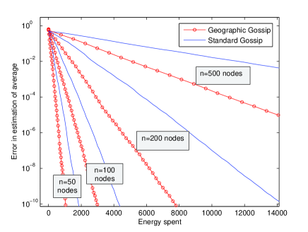
Figure 4: Estimation accuracy versus total spent energy for a linearly varying field.

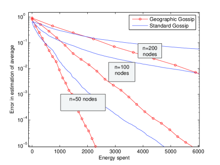
Figure 5: Estimation accuracy versus total spent energy for a smooth field modeling temperature.

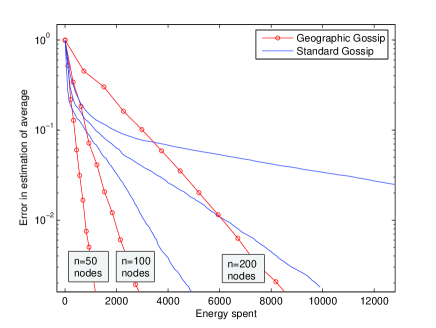
Figure 6: Estimation accuracy versus total spent energy for a field which is zero everywhere except in one node.

5 Conclusions

In this paper we have proposed a novel gossiping algorithm for computing averages in networks in a completely distributed and robust way. Geographic gossip computes the averages faster than standard nearest neighbor gossip because it is using geographic knowledge to quickly diffuse information everywhere in the network. It is not hard to see that our algorithm is efficient for grids (computes the $1/n^{\alpha}$ average in $O(n^{1.5}\log n)$ transmissions) and other topologies that realistically model wireless networks. Even if geographic routing cannot be performed, similar gossip algorithms can be used for any network that can support some form of routing to random nodes. Essentially, we can have nearest-neighbor gossip happening on the overlay network supported by random routing.

The proposed algorithm can be used instead of nearest neighbor gossip in all the schemes that use consensus based aggregation and will greatly reduce the communication cost. For example [19, 18, 21] use similar ideas for localization, Kalman filtering and sensor fusion. In these schemes, geographic gossip can be used instead of standard nearest-neighbor gossip to improve energy consumption.

References

- [1] M. Alanyali, V. Saligrama, and O. Savas, A random-walk model for distributed computation in energy-limited networks, In Proc. of 1st Workshop on Information Theory and its Applications,San Diego, 2006.
- [2] B. Bash and J. C. J.W. Byers. Approximately uniform random sampling in sensor networks. In Proc. of the 1st Workshop on Data Management in Sensor Networks (DMSN ’04), August 2004.
- [3] S. Boyd, A. Ghosh, B. Prabhakar, and D. Shah. Analysis and optimization of randomized gossip algorithms. In Proceedings of the 43rd Conference on Decision and Control (CDC 2004), 2004.
- [4] S. Boyd, A. Ghosh, B. Prabhakar, and D. Shah. Gossip algorithms : Design, analysis and applications. In Proceedings of the 24th Conference of the IEEE Communications Society (INFOCOM 2005), 2005.
- [5] J.-Y. Chen and D. X. G. Pandurangan. Robust aggregates computation in wireless sensor networks: Distributed randomized algorithms and analysis. In 2005 Fourth International Symposium on Information Processing in Sensor Networks (IPSN), 2005.
- [6] P. Flajolet and G. Martin. Probabilistic counting algorithms for data base applications. Journal of Computer and System Sciences, 31(2):182–209, 1985.
- [7] A. E. Gamal, J. Mammen, B. Prabhakar, and D. Shah. Throughput-delay trade-off in wireless networks. In Proceedings of the 24th Conference of the IEEE Communications Society (INFOCOM 2004), 2004.
- [8] P. Gupta and P. Kumar. The capacity of wireless networks. IEEE Transactions on Information Theory, 46(2):388–404, March 2000.
- [9] R. A. Horn and C. R. Johnson. Matrix Analysis. Cambridge University Press, Cambridge, 1987.
- [10] B. Karp and H. Kung. Greedy perimeter stateless routing. In Proceedings of ACM Conf. on Mobile Computing and Networking (MOBICOM), Boston, MA, pages 243–254. ACM, 2000.
- [11] R. Karp, C. Schindelhauer, S. Shenker, and B. Vöcking. Randomized rumor spreading. In Proc. IEEE Conference of Foundations of Computer Science, (FOCS), 2000.
- [12] D. Kempe, A. Dobra, and J. Gehrke. Gossip-based computation of aggregate information. In Proc. IEEE Conference of Foundations of Computer Science, (FOCS), 2003.
- [13] K. Langendoen and N. Reijers. Distributed localization in wireless sensor networks: a quantitative comparison. Computer Networks, 2003.
- [14] C. Moallemi and B. V. Roy. Consensus propagation. Technical report, Stanford University, June 2005.
- [15] D. Mosk-Aoyama and D. Shah. Information dissemination via gossip: Applications to averaging and coding. http://arxiv.org/cs.NI/0504029, April 2005.
- [16] R. Motwani and P. Raghavan. Randomized Algorithms. Cambridge University Press, Cambridge, 1995.
- [17] M. Penrose. Random Geometric Graphs. Oxford studies in probability. Oxford University Press, Oxford, 2003.
- [18] M. Rabbat, R. Nowak, and J. Bucklew, Robust Decentralized Source Localization via Averaging In IEEE International Conference on Acoustics, Speech and Signal processing (ICASSP) , Philadelphia, PA, March 2005.
- [19] D. Spanos, R. Olfati-Saber, and R. Murray. Distributed Kalman filtering in sensor networks with quantifiable performance. In 2005 Fourth International Symposium on Information Processing in Sensor Networks (IPSN), 2005.
- [20] C. H. T. He, B. Blum, J. Stankovic, and T. Abdelzaher. Range-free localization schemes for large scale sensor networks. In Proc. of the 9th annual international conference on Mobile computing and networking, 2003.
- [21] L. Xiao, S. Boyd, and S. Lall. A scheme for asynchronous distributed sensor fusion based on average consensus. In 2005 Fourth International Symposium on Information Processing in Sensor Networks (IPSN), 2005.