Faster Algorithms for Constructing a Concept (Galois) Lattice

Abstract

In this paper, we present a fast algorithm for constructing a concept (Galois) lattice of a binary relation, including computing all concepts and their lattice order. We also present two efficient variants of the algorithm, one for computing all concepts only, and one for constructing a frequent closed itemset lattice. The running time of our algorithms depends on the lattice structure and is faster than all other existing algorithms for these problems.

1 Introduction

Formal Concept Analysis (FCA) [15] has found many applications since its introduction. As the size of datasets grows, such as data generated from high-throughput technologies in bioinformatics, there is a need for efficient algorithms for constructing concept lattices. The input of FCA consists of a triple $({\cal{O}},{\cal{M}},{\cal{I}})$, called context, where ${\cal{O}}$ is a set of objects, ${\cal{M}}$ is a set of attributes, and ${\cal{I}}$ is a binary relation between ${\cal{O}}$ and ${\cal{M}}$. In FCA, the context is structured into a set of concepts. The set of all concepts, when ordered by set-inclusion, satisfies the properties of a complete lattice. The lattice of all concepts is called concept [25] or Galois [10] lattice. When the binary relation is represented as a bipartite graph, each concept corresponds to a maximal bipartite clique (or maximal biclique). There is also a one-one correspondence of a closed itemset [35] studied in data mining and a concept in FCA. The one-one correspondence of all these terminologies – concepts in FCA, maximal bipartite cliques in theoretical computer science (TCS), and closed itemsets in data mining (DM) – was known, e.g. [4, 35]. There is extensive work of the related problems in these three communities, e.g. [3]–[9] in TCS, [11]–[24] in FCA, and [26]–[37] in DM. In general, in TCS, the research focuses on efficiently enumerating all maximal bipartite cliques (of a bipartite graph); in FCA, one is interested in the lattice structure of all concepts; in DM, one is often interested in computing frequent closed itemsets only.

Time complexity.

Given a bipartite graph, it is not difficult to see that there can be exponentially many maximal bipartite cliques. For problems with potentially exponential (in the size of the input) size output, in their seminal paper [7], Johnson et al introduced several notions of polynomial time for algorithms for these problems: polynomial total time, incremental polynomial time, polynomial delay time. An algorithm runs in polynomial total time if the time is bounded by a polynomial in the size of the input and the size of the output. An algorithm runs in incremental polynomial time if the time required to generate a successive output is bounded by the size of input and the size of output generated thus far. An algorithm runs in polynomial delay time if the generation of each output is only polynomial in the size of input. It is not difficult to see that polynomial delay is stronger than incremental polynomial (namely an algorithm with polynomial delay time is also running in incremental polynomial), which is stronger than polynomial total time. polynomial delay algorithm, we can further distinguish if the space used is polynomial or exponential in the input size.

Previous work.

Observe that the maximal bipartite clique (MBC) problem is a special case of the maximal clique problem in a general graph. Namely, given a bipartite graph $G=(V_{1},V_{2},E)$, a maximal bipartite clique corresponds to a maximal clique in $\breve{G}=(V_{1}\cup V_{2},\breve{E})$ where $\breve{E}=E\cup(V_{1}\times V_{1})\cup(V_{2}\times V_{2})$. Consequently, any algorithm for enumerating all maximal cliques in a general graph, e.g., [9, 7], also solves the MBC problem. In fact, the best known algorithm in enumerating all maximal bipartite cliques, which was proposed by Makino and Uno [8] that takes $O(\Delta^{2})$ polynomial delay time where $\Delta$ is the maximum degree of $G$, was based on this approach. The fact that the set of maximal bipartite cliques constitutes a lattice was not observed in the paper and thus the property was not utilized for the enumeration algorithm.

In FCA, much of research has been devoted to study the properties of the lattice structure. There are several algorithms, e.g. [20, 24, 19], that construct the lattice, i.e. computing all concepts together with its lattice order. There are also some algorithms that compute only concepts, e.g. [22, 15]. (We remark that the idea of using a total lectical order on concepts Ganter’s algorithm  [15] is also used in [7, 8] for enumerating maximal (bi)cliques.) See [17] for a comparison studies of these algorithms. The best polynomial total time algorithm was by Nourine and Raynaud [20] with $O(nm|{\cal{B}}|)$ time and $O(n|{\cal{B}}|)$ space, where $n=|{\cal{O}}|$ and $m=|{\cal{M}}|$ and ${\cal{B}}$ denote the set of all concepts. This algorithm can be easily modified to run in $O(mn)$ incremental time [21]. Observe that the space of total size of all concepts is needed if one is to keep the entire structure explicitly. There were several other algorithms, e.g.[15, 19], all run in $O(n^{2}m)$ polynomial delay. There is another algorithm [24] that is based on divide-and-conquer approach, but the analytical running time of the algorithm is unknown as it is difficult to analyze.

There are several algorithms in data mining for computing frequent closed itemsets, such as CHARM(-L) [36, 37], and CLOSET(+) [30, 33]. To our best knowledge, the algorithm with theoretical analysis running time was given in [4] with $O(m^{2}n)$ incremental polynomial running time, where $n=|{\cal{O}}|$ and $m=|{\cal{M}}|$.

Our Results.

In this paper, by making use of the lattice structure of concepts, we present a simple and fast algorithm for computing all concepts together with its lattice order. The main idea of the algorithm is that given a concept, when all of its successors are considered together (i.e. in a batch manner), they can be efficiently computed. We compute concepts in the Breadth First Search (BFS) order – the ordering given by BFS traversal of the lattice. When computing the concepts in this way, not only do we compute all concepts but also we identify all successors of each concept. Another idea of the algorithm is that we make use of the concepts generated to dynamically update the adjacency relations. The running time of our algorithm is $O(\sum_{a\in\mathsf{ext}(C)}|\mathsf{cnbr}(a)|)$ polynomial delay for each concept $C$ (see Section 2 for related background and terminology), where $\mathsf{cnbr}(a)$ is the reduced adjacency list of $a$. Our algorithm is faster than the best known algorithms for constructing a lattice because the algorithm is faster than a basic algorithm that runs in $O(\sum_{a\in\mathsf{ext}(C)}|\mathsf{nbr}(a)|)$, where $|\mathsf{nbr}(a)|$ is number of attributes adjacent to the object $a$, and this basic algorithm is already as fast as the current best algorithms for the problem.

We also present two variants of the algorithm: one is computing all concepts only and another is constructing the frequent closed itemset lattice. Both algorithms are faster than the current start-of-the-art program for these problems.

Outline.

The paper is organized as follows. In Section 2, we review some background and notation on FCA. In Section 3, we describe some basic properties of concepts that we use in our lattice-construction algorithm. In Section 4, we first describe the high level idea of our algorithm. Then we describe how to efficiently implement the algorithm. In Section 5, we describe two variants of the algorithm. One is for computing all concepts only and another is for constructing a frequent closed itemset lattice. We conclude with discussion in Section 6.

2 Background and Terminology on FCA

In FCA, a triple $({\cal{O}},{\cal{M}},{\cal{I}})$ is called a context, where ${\cal{O}}=\{g_{1},g_{2},\ldots,g_{n}\}$ is a set of $n$ elements, called objects; ${\cal{M}}=\{1,2,\ldots,m\}$ is a set of $m$ elements, called attributes; and ${\cal{I}}\subseteq{\cal{O}}\times{\cal{M}}$ is a binary relation. The context is often represented by a cross-table as shown in Figure 1. A set $X\subseteq{\cal{O}}$ is called an object set, and a set $J\subseteq{\cal{M}}$ is called an attribute set. Following the convention, we write an object set $\{a,c,e\}$ as $ace$, and an attribute set $\{1,3,4\}$ as $134$.

For $i\in{\cal{M}}$, denote the adjacency list of $i$ by $\mathsf{nbr}(i)=\{g\in{\cal{O}}:(g,i)\in{\cal{I}}\}$. Similarly, for $g\in{\cal{O}}$, denote the adjacency list of $g$ by $\mathsf{nbr}(g)=\{i\in{\cal{M}}:(g,i)\in{\cal{I}}\}$.

Definition 1

The function $\mathsf{attr}:2^{{\cal{O}}}\longrightarrow 2^{{\cal{M}}}$ maps a set of objects to their common attributes: $\mathsf{attr}(X)=\cap_{g\in X}\mathsf{nbr}(g)$, for $X\subseteq{\cal{O}}$. The function $\mathsf{obj}:2^{{\cal{M}}}\longrightarrow 2^{{\cal{O}}}$ maps a set of attributes to their common objects: $\mathsf{obj}(J)=\cap_{j\in J}\mathsf{nbr}(j)$, for $J\subseteq{\cal{M}}$.

It is easy to check that for $X\subseteq{\cal{O}}$, $X\subseteq\mathsf{obj}(\mathsf{attr}(X))$, and for $J\subseteq{\cal{M}}$, $J\subseteq\mathsf{attr}(\mathsf{obj}(J))$.

Definition 2

An object set $X\subseteq{\cal{O}}$ is closed if $X=\mathsf{obj}(\mathsf{attr}(X))$. An attribute set $J\subseteq{\cal{M}}$ is closed if $J=\mathsf{attr}(\mathsf{obj}(J))$.

The composition of $\mathsf{obj}$ and $\mathsf{attr}$ induces a Galois connection between $2^{{\cal{O}}}$ and $2^{{\cal{M}}}$. Readers are referred to [15] for properties of the Galois connection.

Definition 3

A pair $C=(A,B)$, with $A\subseteq{\cal{O}}$ and $B\subseteq{\cal{M}}$, is called a concept if $A=\mathsf{attr}(B)$ and $B=\mathsf{obj}(A)$.

For a concept $C=(A,B)$, by definition, both $A$ and $B$ are closed. The object set $A$ is called the extent of $C$, written as $A=\mathsf{ext}(C)$, and the attribute set $B$ is called the intent of $C$, and written as $B=\mathsf{int}(C)$. The set of all concepts of the context $({\cal{O}},{\cal{M}},{\cal{I}})$ is denoted by ${\cal{B}}({\cal{O}},{\cal{M}},{\cal{I}})$ or simply ${\cal{B}}$ when the context is understood.

Let $(A_{1},B_{1})$ and $(A_{2},B_{2})$ be two concepts in ${\cal{B}}$. Observe that if $A_{1}\subseteq A_{2}$, then $B_{2}\subseteq B_{1}$. We order the concepts in ${\cal{B}}$ by the following relation $\prec$:

$$(A_{1},B_{1})\prec(A_{2},B_{2})\Longleftrightarrow A_{1}\subseteq A_{2}(B_{2}\subseteq B_{1}).$$

It is not difficult to see that the relation $\prec$ is a partial order on ${\cal{B}}$. In fact, ${\cal{L}}=<{\cal{B}},\prec>$ is a complete lattice and it is known as the concept or Galois lattice of the context $({\cal{O}},{\cal{M}},{\cal{I}})$. For $C,D\in{\cal{B}}$ with $C\prec D$, if for all $E\in{\cal{B}}$ such that $C\prec E\prec D$ implies that $E=C$ or $E=D$, then $C$ is called the successor (or lower neighbor) of $D$, and $D$ is called the predecessor (or upper neighbor) of $C$ . The diagram representing an ordered set (where only successors/predecessors are connected by edges) is called a Hasse diagram (or a line diagram). See Figure 1 for an example of the line diagram of a Galois lattice.

For a concept $C=(\mathsf{ext}(C),\mathsf{int}(C))$, $\mathsf{ext}(C)=\mathsf{obj}(\mathsf{int}(C))$ and $\mathsf{int}(C)=\mathsf{attr}(\mathsf{ext}(C))$. Thus, $C$ is uniquely determined by either its extent, $\mathsf{ext}(C)$, or by its intent, $\mathsf{int}(C)$. We denote the concepts restricted to the objects ${\cal{O}}$ by ${\cal{B}}_{{\cal{O}}}=\{\mathsf{ext}(C):C\in{\cal{B}}\}$, and the attributes ${\cal{M}}$ by ${\cal{B}}_{{\cal{M}}}=\{\mathsf{int}(C):C\in{\cal{B}}\}.$ For $A\in{\cal{B}}_{{\cal{O}}}$, the corresponding concept is $(A,\mathsf{attr}(A))$. For $J\in{\cal{B}}_{{\cal{M}}}$, the corresponding concept is $(\mathsf{obj}(J),J)$. The order $\prec$ is completely determined by the inclusion order on $2^{{\cal{O}}}$ or equivalently by the reverse inclusion order on $2^{{\cal{M}}}$. That is, ${\cal{L}}=<{\cal{B}},\prec>$ and ${\cal{L}}_{{\cal{M}}}=<{\cal{B}}_{{\cal{M}}},\supseteq>$ are order-isomorphic. We have the property that $(\mathsf{obj}(Z),Z)$ is a successor of $(\mathsf{obj}(X),X)$ in ${\cal{L}}$ if and only if $Z$ is a successor of $X$ in ${\cal{L}}_{{\cal{M}}}$. Since the set of all concepts is finite, the lattice order relation is completely determined by the covering (successor/predecessor) relation. Thus, to construct the lattice, it is sufficient to compute all concepts and identify all successors of each concept.

3 Basic Properties

In this section, we describe some basic properties of the concepts on which our lattice construction algorithms are based.

Proposition 1

Let $C$ be a concept in ${\cal{B}}({\cal{O}},{\cal{M}},{\cal{I}})$. For $i\in{\cal{M}}\setminus\mathsf{int}(C)$, if $E_{i}=\mathsf{ext}(C)\cap\mathsf{nbr}(i)$ is not empty, $E_{i}$ is closed. Consequently, $(E_{i},\mathsf{attr}(E_{i}))$ is a concept.

Proof

For $i\in{\cal{M}}\setminus\mathsf{int}(C)$, suppose that $E_{i}=\mathsf{ext}(C)\cap\mathsf{nbr}(i)$ is not empty. We will show that $\mathsf{obj}(\mathsf{attr}(E_{i}))=E_{i}$. Since $E_{i}\subseteq\mathsf{obj}(\mathsf{attr}(E_{i}))$, it remains to show that $\mathsf{obj}(\mathsf{attr}(E_{i}))\subseteq E_{i}$. By definition, $\mathsf{obj}(\mathsf{int}(C)\cup\{i\})=(\cap_{j\in\mathsf{int}(C)}\mathsf{nbr}(j))\cap\mathsf{nbr}(i)=\mathsf{ext}(C)\cap\mathsf{nbr}(i)=E_{i}$. Thus, $(\mathsf{int}(C)\cup\{i\})\subseteq\mathsf{attr}(\mathsf{obj}(\mathsf{int}(C)\cup\{i\}))=\mathsf{attr}(E_{i})$. Consequently, $\mathsf{obj}(\mathsf{attr}(E_{i}))\subseteq\mathsf{obj}(\mathsf{int}(C)\cup\{i\})=E_{i}$.

1 2 3 4 a $\times$ $\times$ b $\times$ $\times$ $\times$ c $\times$ $\times$ d $\times$ $\times$
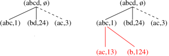
(a)	(b)	(c)

Figure 1: (a) A context $({\cal{O}},{\cal{M}},{\cal{I}})$ with ${\cal{O}}=\{a,b,c,d\}$ and ${\cal{M}}=\{1,2,3,4\}$. The cross $\times$ indicates a pair in the relation ${\cal{I}}$. (b) The corresponding Galois/concept lattice. (c) $\mathsf{Child}(abcd,\emptyset)=\{(abc,1),(bd,24),(ac,3)\}$; $\mathsf{Child}(abc,1)=\{(ac,13),(b,124)\}$.

Example. Consider the concept $C=(abcd,\emptyset)$ of context in Figure 1, we have $E_{1}=abc,E_{2}=bd,E_{3}=ac,E_{4}=bd$.

3.1 Defining the equivalence classes

For a closed attribute set $X\subset{\cal{M}}$, denote the set of remaining attributes $\{i\in{\cal{M}}\setminus X:\mathsf{obj}(X)\cap\mathsf{nbr}(i)\neq\emptyset\}$ by $\mathsf{res}(X)$. Consider the following equivalence relation $\sim$ on $\mathsf{res}(X)$: $i\sim j\Longleftrightarrow\mathsf{obj}(X)\cap\mathsf{nbr}(i)=\mathsf{obj}(X)\cap\mathsf{nbr}(j)$, for $i\neq j\in\mathsf{res}(X)$.

Let $S_{1},\ldots,S_{t}$ be the equivalence classes induced by $\sim$, i.e. $\mathsf{res}(X)=S_{1}\cup\ldots\cup S_{t}$, and $\mathsf{obj}(X)\cap\mathsf{nbr}(i)=\mathsf{obj}(X)\cap\mathsf{nbr}(j)$ for any $i\neq j\in S_{k}$, $1\leq k\leq t$. We denote the set $\{S_{1},\ldots,S_{t}\}$ by $\mathsf{AttrChild}(X)$. We call $S_{j}$ the sibling of $S_{i}$ for $j\neq i$. For convenience, we will write $X\cup S_{i}$ by $XS_{i}$. When there is no confusion, we abuse the notation by writing $X\cup\mathsf{AttrChild}(X)=\{XS:S\in\mathsf{AttrChild}(X)\}$. Note that by definition, $\mathsf{obj}(XS_{k})=\mathsf{obj}(X)\cap\mathsf{obj}(S_{k})=\mathsf{obj}(X)\cap\mathsf{nbr}(i)$ for some $i\in S_{k}$. We denote the pairs $\{(\mathsf{obj}(XS_{1}),XS_{1}),\ldots,(\mathsf{obj}(XS_{1}),XS_{1})\}$ by $\mathsf{Child}(\mathsf{obj}(X),X)$.

Recall that ${\cal{L}}=<{\cal{B}},\prec>$ and ${\cal{L}}_{{\cal{M}}}=<{\cal{B}}_{{\cal{M}}},\supseteq>$ are order-isomorphic. We have the property that $(\mathsf{obj}(Y),Y)$ is a successor of $(\mathsf{obj}(X),X)$ in ${\cal{L}}$ if and only if $Y$ is a successor of $X$ in ${\cal{L}}_{{\cal{M}}}$. For each $S\in\mathsf{AttrChild}(X)$, we call $XS$ a child of $X$ and $X$ a parent of $XS$. By the definition of the equivalence class, for each $Z$ that is a successor of $X$, there exists a $S\in\mathsf{AttrChild}(X)$ such that $Z=XS$. That is, if $Z$ is a successor of $X$, $Z$ is a child of $X$.

Let $\mathsf{Succ}(X)$ denote all the successors of $X$, then we have $\mathsf{Succ}(X)\subseteq X\cup\mathsf{AttrChild}(X)$. However, not every child of $X$ is a successor of $X$. For the example in Figure 1, $\mathsf{AttrChild}(\emptyset)=\{1,24,3\}$, where $1$ and $24$ are successors of $\emptyset$ but $3$ is not. $\mathsf{Succ}(\emptyset)=\{1,24\}\subset\mathsf{AttrChild}(\emptyset)$; while $\mathsf{AttrChild}(1)=\{24,3\}$, $\mathsf{Succ}(a)=\{124,13\}=1\cup\mathsf{AttrChild}(1)$. Similarly, if $P$ is a predecessor of $X$, then P is parent of $X$ but it is not necessary that every parent of $X$ is a predecessor of $X$.

Note that for $S\in\mathsf{AttrChild}(X)$, if $XS\in\mathsf{Succ}(X)$, then by definition $XS$ is closed. It is easy to check that the converse is also true. Namely, if $XS$ is closed, then $XS\in\mathsf{Succ}(X)$. In other words, we have the following proposition.

Proposition 2

$\mathsf{Succ}(X)=\{XS:XS$ is closed, $S\in\mathsf{AttrChild}(X)\}$.

3.2 Characterizations of Closure

By definition, an attribute set $X$ is closed if $\mathsf{obj}(\mathsf{attr}(X))=X$. In the following we give two characterizations for an attribute set being closed based on its relationship with its siblings.

Proposition 3

For $S\in\mathsf{AttrChild}(X)$, $XS$ is not closed if and only if there exists $T\in\mathsf{AttrChild}(X)$, $T\neq S$, such that $\mathsf{obj}(XS)\subset\mathsf{obj}(XT)$. Furthermore, for all $T\in\mathsf{AttrChild}(X)$ with $\mathsf{obj}(XS)\subset\mathsf{obj}(XT)$, there exists $S^{\prime}\in\mathsf{AttrChild}(XT)$ such that $S\subseteq S^{\prime}$, $\mathsf{obj}(XS)=\mathsf{obj}(XTS^{\prime})$ and $XS\subset XTS^{\prime}$.

Proof

If $XS$ is not closed, by definition, there exists $i\in\mathsf{res}(X)\setminus S$ such that $i\in\mathsf{attr}(\mathsf{obj}(XS))$. As $\mathsf{AttrChild}(X)$ is a partition of $\mathsf{res}(X)$, there exists a $T\in\mathsf{AttrChild}(X)$ such that $i\in T$, and thus $\mathsf{obj}(XT)=\mathsf{obj}(X)\cap\mathsf{nbr}(i)\supset\mathsf{obj}(XS)$.

Conversely, suppose there exists $T\in\mathsf{AttrChild}(X)$ such that $\mathsf{obj}(XS)\subset\mathsf{obj}(XT)$. Then $\mathsf{attr}(\mathsf{obj}(XS))\supseteq XTS$. That is, $XS\subset XTS\subseteq\mathsf{attr}(\mathsf{obj}(XS))$, which implies $XS$ is not closed.

Suppose that $\mathsf{obj}(XS)\subset\mathsf{obj}(XT)$ with $T\in\mathsf{AttrChild}(X)$. For $i\in S$, $\mathsf{obj}(XT)\cap\mathsf{nbr}(i)=\mathsf{obj}(XT)\cap\mathsf{obj}(X)\cap\mathsf{nbr}(i)=\mathsf{obj}(XT)\cap\mathsf{obj}(XS)=\mathsf{obj}(XS)$. Thus, there exists $S^{\prime}\in\mathsf{AttrChild}(XT)$ such that $S\subseteq S^{\prime}$, $\mathsf{obj}(XS)=\mathsf{obj}(XTS^{\prime})$. Since $X,S,T$ are disjoint, $XS\subset XTS\subseteq XTS^{\prime}$.

Based on the first part of this proposition (first characterization), we can test if $XS$ is closed, for $S\in\mathsf{AttrChild}(X)$, by using subset testing of its object set against its siblings’ object set. Namely, $XS$ is closed if and only $\mathsf{obj}(XS)$ is not a proper subset of its siblings’ object set. In our running example in Figure 1, $3$ is not closed because its object set $\mathsf{obj}(3)=ac$ is a proper subset of the object set of its sibling, $\mathsf{obj}(1)=abc$.

In general, subset testing operations are expensive. We, however, can make use of the second part of the proposition (second characterization) for testing closure using set exact matching operations instead of subset testing operations. This is because if we process the children in the decreasing order of their object-set size, we can test the closure of $XS$ by comparing its size against the size of the attribute set (if exists) of $\mathsf{obj}(XS)$. Namely, we first search if $\mathsf{obj}(XS)$ exists by a set exact matching operation. If it does not, then $XS$ is closed. Otherwise, if the size of the existing attribute set of $\mathsf{obj}(XS)$ is greater than $|XS|$, then $XS$ is not closed. In our running example, $3$ is not closed because $\mathsf{obj}(3)=ac$ has a larger attribute set $13$.

4 Algorithm: Constructing a Concept/Galois Lattice

In this section, we first describe the algorithm in general terms, independent of the implementation details. We then show how the algorithm can be implemented efficiently.

4.1 High Level Idea

Recall that constructing a concept lattice includes generating all concepts and identifying each concept’s successors.

Our algorithm starts with the top concept $({\cal{O}},\mathsf{attr}({\cal{O}}))$. We process the concept by computing all its successors, and then recursively process each successor by either the Depth First Search (DFS) order — the ordering obtained by DFS traversal of the lattice — or Breadth First Search (BFS) order. According to Proposition 2, successors of a concept can be computed from its children. Let $C=(\mathsf{obj}(X),X)$ be a concept. First, we compute all the children $\mathsf{Child}(C)=\{(\mathsf{obj}(XS),XS):S\in\mathsf{AttrChild}(X)\}$. Then for each $S\in\mathsf{AttrChild}(X)$, we check if $XS$ is closed. If $XS$ is closed, $(\mathsf{obj}(XS),XS)$ is a successor of $C$. Since a concept can have several predecessors, it can be generated several times. We check its existence to make sure that each concept is processed once and only once. The pseudo-code of the algorithm based on BFS is shown in Algorithm 1.

Algorithm 1 Concept-Lattice Construction – BFS

1:

2:Compute the top concept $C=({\cal{O}},\mathsf{attr}({\cal{O}}))$;

3:

4:Initialize a queue $Q=\{C\}$;

5:

6:Compute $\mathsf{Child}(C)$;

7:

8:while $Q$ is not empty do

9:

10:$C=\mbox{ dequeue}(Q)$;

11:Let $X=\mathsf{int}(C)$ and suppose $\mathsf{AttrChild}(X)=<S_{1},S_{2},\ldots,S_{k}>$;

12:

13:for $i=1$ to $k$ do

14:

15:if $XS_{i}$ is closed then

16:Denote the concept $(\mathsf{obj}(XS_{i}),XS_{i})$ by $K$;

17:

18:if K does not exist then

19:

20:Compute $\mathsf{Child}(K)$;

21:

22:Enqueue $K$ to $Q$;

23:end if

24:

25:Identify $K$ as a successor of $C$;

26:end if

27:end for

28:end while

4.2 Implementation

The efficiency of the algorithm depends on the efficient implementation of processing a concept that include three procedures: (1) computing $\mathsf{Child}()$; (2)testing if an attribute set is closed; (3) testing if a concept already exists.

First, we describe how to compute $\mathsf{Child}(\mathsf{obj}(X),X)$ in $O(\sum_{a\in\mathsf{obj}(X)}|\mathsf{nbr}(a)|)$ time, using a procedure, called Sprout, described in the following lemma.

Lemma 1

For $(\mathsf{obj}(X),X)\in{\cal{B}}$, it takes $O(\sum_{a\in\mathsf{obj}(X)}|\mathsf{nbr}(a)|)$ to compute $\mathsf{Child}(\mathsf{obj}(X),X)$.

Proof

Let $\mathsf{res}(X)=\cup_{a\in\mathsf{obj}(X)}\mathsf{nbr}(a)\setminus X$. For each $i\in\mathsf{res}(X)$, we associate it with a set $E_{i}$ (which is initialized as an empty set). For each object $a\in\mathsf{obj}(X)$, we scan through each attribute $i$ in its neighbor list $\mathsf{nbr}(a)$, append $a$ to the set $E_{i}$. This step takes $O(\sum_{a\in\mathsf{obj}(X)}|\mathsf{nbr}(a)|)$. Next we collect all the sets $\{E_{i}:i\in\mathsf{res}(X)\}$. We use a trie to group the same object set: search $E_{i}$ in the trie; if not found, insert $E_{i}$ into the trie with $\{i\}$ as its attribute set, otherwise we append $i$ to $E_{i}$’s existing attribute set. This step takes $O(\sum_{i\in\mathsf{res}(X)}|E_{i}|)=O(\sum_{a\in\mathsf{obj}(X)}|\mathsf{nbr}(a)|)$. Thus, this procedure, called Sprout$(\mathsf{obj}(X),X)$, takes $O(\sum_{a\in\mathsf{obj}(X)}|\mathsf{nbr}(a)|)$ time to compute $\mathsf{Child}(\mathsf{obj}(X),X)$.

For $S\in\mathsf{AttrChild}(X)$, we test if $XS$ is closed based on the second characterization in Proposition 3. For this method to work, it requires processing the children $\mathsf{Child}(\mathsf{obj}(X),X)$ in the decreasing order of their object-set size. Suppose $\mathsf{AttrChild}(X)=\{S_{1},\ldots,S_{k}\}$ where $|\mathsf{obj}(XS_{1})|\geq|\mathsf{obj}(XS_{2})|\geq\ldots\geq|\mathsf{obj}(XS_{k})|$. We process $S_{i-1}$ before $S_{i}$. If $XS_{i-1}$ is closed, we also compute its children $\mathsf{Child}(\mathsf{obj}(XS_{i-1}),XS_{i-1})$. Now to test if $XS_{i}$ is closed, we check if $\mathsf{obj}(XS_{i})$ exists. If it does not, then $XS_{i}$ is closed. Otherwise, we compare $|XS_{i}|$ against the size of the existing attribute set of $\mathsf{obj}(XS_{i})$. If $|XS_{i}|$ is not smaller, then $XS_{i}$ is closed otherwise it is not. To efficiently search $\mathsf{obj}(XS_{i})$, we use a trie (with hashing over each node) to store the object sets of concepts generated so far and it takes linear time to search and insert (if not exists) an object set. That is, it will take $O(|\mathsf{obj}(XS_{i})|)$ time to check if $XS_{i}$ is closed. The total time it takes to check if all children are closed is $O(\sum_{i=1}^{k}|\mathsf{obj}(XS_{i})|)$.

Recall that a concept $C=(\mathsf{obj}(X),X)$ is uniquely determined by its extent $\mathsf{obj}(X)$ or its intent $X$. Therefore, we can store either the object sets or the attribute sets generated so far in a trie, and then test the existence of $C$ by testing the existence of $\mathsf{obj}(X)$ or $X$. Since searching the object sets are needed in testing the closure of an attribute set as described above, the cost of testing the existence $\mathsf{obj}(X)$ comes for free.

Note that $\sum_{a\in\mathsf{obj}(X)}|\mathsf{nbr}(a)|>\sum_{i=1}^{k}|\mathsf{obj}(XS_{i})|\cdot|S_{i}|$. Hence, the time it takes to process a concept is dominated by the procedure Sprout, in $O(\sum_{a\in\mathsf{obj}(X)}|\mathsf{nbr}(a)|)$ time. If we can reduce the sizes of the adjacency lists ($|\mathsf{nbr}()|$), we can reduce the running time of the algorithm. Note that this basic algorithm is already as fast as any existing algorithm for constructing a concept lattice (or computing all concepts only that takes $O(\Delta^{2})$ time where $\Delta$ is the maximum size of adjacency lists).

In the following we describe how to dynamically update the adjacency lists that will reduce the sizes of adjacent lists, and thus improve the running time of the algorithm.

4.2.1 Further Improvement: Dynamically Update Adjacency Lists.

Consider a concept $C=(\mathsf{obj}(X),X)$, the object sets of all descendants of $C$ are all subsets of $\mathsf{obj}(X)$. To compute the descendants of $C$, it suffices to consider the objects with restriction to $\mathsf{obj}(X)$. For $S\in\mathsf{AttrChild}(X)$, by definition, all attributes in $S$ have the same adjacency lists when restricting to $\mathsf{obj}(X)$. That is, for all $i\neq j\in S$, $\mathsf{nbr}(i)\cap\mathsf{obj}(X)=\mathsf{nbr}(j)\cap\mathsf{obj}(X)(=\mathsf{obj}(XS))$. In other words, for all $a\in\mathsf{obj}(X)$, $i\in\mathsf{nbr}(a)\Leftrightarrow j\in\mathsf{nbr}(a)$, for all $i,j\in S$, i.e., the adjacent list of $a$ either contains all elements in $S$ or no element in $S$. Therefore, we can reduce the sizes of adjacent lists of objects by representing all attributes in $S$ by a single element. For example in Figure example2, we can use a single element $16$ to represent the two attributes $1$ and $6$, and $35$ to represent $3$ and $5$. In doing so, we reduce the size of adjacency list of $b$ from $5$ elements $\{1,3,4,5,6\}$ to three elements $\{16,35,4\}$. We call the reduced adjacency lists the condensed adjacency lists. Denoted the condensed adjacent list by $\mathsf{cnbr}()$. The set of condensed adjacency lists corresponds to a reduced cross-table. For example, the reduced cross table of $\mathsf{Child}(abcde,\emptyset)$ of the above example is shown in Figure 2.

1 2 3 4 5 6 7 a $\times$ $\times$ b $\times$ $\times$ $\times$ $\times$ $\times$ c $\times$ $\times$ $\times$ d $\times$ $\times$ $\times$ e $\times$ $\times$		16 2 35 4 7 a $\times$ b $\times$ $\times$ $\times$ c $\times$ $\times$ d $\times$ $\times$ e $\times$ $\times$
(a)	(b)	(c)

Figure 2: (a) A context. (b) The corresponding concept lattice. (c) Reduced cross-table of $\mathsf{Child}(abcde,\emptyset)$ of the context.

In order to use the condensed adjacency lists in procedure Sprout, we need to process our concepts in BFS order and it requires one extra level, i.e. in a two-level manner. More specifically, for a concept $C=(\mathsf{obj}(X),X)$, we first compute all its children $\mathsf{Child}(C)$. Then we dynamically update the adjacency lists by representing the attributes in each child of $C$ with one single element. We then use these condensed adjacency lists to process each child of $C$. That is, instead of using the global adjacency lists, when processing $(\mathsf{obj}(XS),XS)$, we use the condensed adjacency lists of its parent. It takes $O(\sum_{S\in\mathsf{AttrChild}(X)}|\mathsf{obj}(XS)|)$ for $C$ to generate its condensed adjacency lists $\mathsf{cnbr}()$ (see Algorithm 3 in the Appendix for the pseudo-code). And the time for the procedure Sprout is $O(\sum_{a\in\mathsf{obj}(X)}|\mathsf{cnbr}(a)|)$ (see Algorithm 2 in the Appendix for the pseudo-code). Notice that $\sum_{a\in\mathsf{obj}(X)}|\mathsf{cnbr}(a)|>\sum_{S\in\mathsf{AttrChild}(X)}|\mathsf{obj}(XS)|$, the time for updating the adjacency lists is subsumed by the time required for procedure Sprout. Therefore, our new running time is $O(\sum_{a\in\mathsf{obj}(X)}|\mathsf{cnbr}(a)|)$ for each concept $(\mathsf{obj}(X),X)$. See Algorithm 4 for the pseudo-code and Figure 3 for a step-by-step illustration of the algorithm.

5 Variants of The Algorithm

For some applications, one is not interested in the entire concept lattice. In the following, we will describe how to modify our algorithm to solve two special cases: enumerating all concepts only and constructing a frequent closed itemset lattice.

5.1 Algorithm 2: Computing All Concepts or Maximal Bipartite Cliques

If one is interested in computing all the concepts and not in their lattice order, as in enumerating all maximal bicliques studied in [8]. We can easily modify our algorithm to give an even faster algorithm for this purpose. This is because in our algorithm, each concept is generated many times, more precisely, at least number of its predecessors times. For example in Figure 3, $(d,235)$ is generated twice, one by each of its predecessor. However, when we need all concepts only, we do not need regenerate the concepts again and again. This can be easily accomplished by considering the right siblings only in the procedure Sprout, i.e. changing the line 3 to $\mathsf{for}~{}~{}i\in\mathsf{nbr}(a)\mbox{ AND }i>s~{}~{}\mathsf{do}$, while the other parts of the algorithm remain the same. Depending on the lattice structure, this can significantly speed up the algorithm as the number of siblings is decreasing in a cascading fashion. A more careful analysis is needed for the running time of this algorithm.

5.2 Algorithm 3: Constructing a Closed Itemset Lattice

In data mining, one is interested in large concepts, i.e. $(\mathsf{obj}(X),X)$ where $|\mathsf{obj}(X)|$ is larger than a threshold. Although our algorithm can naturally be modified to construct such a closed itemset lattice: we stop processing a concept when the size of its object set is less than the given threshold, where objects correspond to transactions and attributes correspond to items. Theoretically, when the memory requirement is not a concern, our algorithm is faster than all other existing algorithms (including the state-of-art program CHARM-L) for constructing such a frequent closed itemset lattice. However, in practice, for large data sets (as those studied in data mining), the data structure – a trie on objects (transactions) – requires huge memory and this may threaten the algorithm’s practical efficiency. However, it is not difficult to modify our algorithm so that a trie on attributes (items) instead is used. Recall that a trie on objects are required in two steps of our algorithm: testing the closure of an attribute set and testing the existence of a concept. As noted above, the existence of a concept can also be tested on its intent (i.e. attributes), thus we can use a trie on attributes for testing the existence of a concept. To avoid using a trie on objects for testing the closure of an attribute set, we can use the first characterization in Proposition 3 instead, that is, we test the closure of an attribute set by using subset testing of its object set against its siblings’ object set, as described in Section 3. Further, we can employ the practically efficient technique diffset as in CHARM(-L) for both our Sprout procedure and subset testing operations. We are testing the performance of the diffset based implementation on the available benchmarks and the results will be reported elsewhere.

6 Discussion

Our interest in FCA stems from our research in microarray data analysis [2]. We have implemented an not yet optimized version of our algorithm (with less than 500 effective lines in C++). The program is very efficient for our applications, in which our data consists of about 10000 objects and 29 attributes. It took less than 1 second for the program to produce the concept lattice (about 530 vertices/concepts and 1500 edges) in a Pentium IV 3.0GHz computer with 2G memory running under Fedora 2 linux OS. The program is available upon request at this point and will release to the public in the near future.

As FCA finds more and more applications, especially in bioinformatics, efficient algorithms for constructing concept/Galois lattices are much needed. Our algorithm is faster than the existing algorithms for this problem, nevertheless, it seems to have much room to improve.

Appendix

$$\begin{array}[]{l@{\quad\quad\quad}l}(1)\mathsf{Sprout}(abcde,\emptyset):&(2)\mathsf{Sprout}(abc,16)\\ \psfig{width=166.2212pt}&\psfig{width=166.2212pt}\\ \\ (3)\mbox{Eliminate }(bc,4)\mbox{ as it is not closed}&(4)\mathsf{Sprout}(bd,35)\\ \psfig{width=166.2212pt}&\psfig{width=166.2212pt}\\ \\ (5)\mathsf{Sprout}(de,2)&(6)\mathsf{Sprout}(bc,146)\\ \psfig{width=166.2212pt}&\psfig{width=166.2212pt}\\ \\ (7)\mbox{Eliminate }(b,1356)\mbox{ as it is not closed}&(8)\mathsf{Sprout}(b,13456),(d,235),(e,27)\\ \psfig{width=166.2212pt}&\psfig{width=166.2212pt}\\ \end{array}$$

Figure 3: Step by step illustration of the 2-level BFS lattice construction algorithm. The context and the corresponding lattice are shown in Figure 2.

Algorithm 2 Sprout

1:Input: $s$, $\mathsf{content}$ and $\mathsf{nbr}$

2:$(\mathsf{obj}(X),X)$ is the $s$th child of $G$. Let $K=\{1,\ldots,k\}$ be all the children of $G$.

3:Output: $\mathsf{Child}(\mathsf{obj}(X),X)=\{(\mathsf{obj}(XS_{i}),XS_{i}):1\leq i\leq t\}$

4:

5:For each $i\in K$, set $C_{i}=\emptyset$.

6:

7:for $a\in C$ do

8:

9:for $i\in\mathsf{nbr}(a)\setminus\{s\}$ do

10:

11:Append $a$ to $C_{i}$;

12:end for

13:end for

14:The following takes $O(\sum_{i\in K}|C_{i}|)=O(\sum_{a\in C}|\mathsf{nbr}(a)|)$ time.

15:

16:Initialize a local trie $T_{C}$ over objects;

17:

18:for $i\in K$ do

19:

20:if $C_{i}$ does not exist in $T_{C}$ then

21:

22:Insert $C_{i}$ into $T_{C}$;

23:

24:$S_{i}=\mathsf{content}(i)$;

25:

26:else

27:

28:Merge $S_{i}$ with $\mathsf{content}(i)$ ;

29:end if

30:end for

31:

32:Output all the pairs in $T_{C}$: $\{(\mathsf{obj}(XS_{j}),XS_{j}):1\leq j\leq t\}$.

Algorithm 3 CondenseAdjacentlists

1:Input: $\mathsf{Child}(C)=\{(\mathsf{obj}(XS_{i}),XS_{i}):1\leq i\leq t\}$

2:Output: $\mathsf{content}(i)$ for $i=1\ldots t$, and new adjacency lists, $\mathsf{nbr}(a)$, $a\in\mathsf{obj}(X)$

3:

4:For each $a\in\mathsf{obj}(X)$, $\mathsf{nbr}(a)=\emptyset$;

5:

6:for $i=1$ to $t$ do

7:

8:$\mathsf{content}(i)=S_{i}$;

9:

10:for each $a\in\mathsf{obj}(XS_{i})$, append $i$ to $\mathsf{nbr}(a)$;

11:end for

Algorithm 4 Concept-Lattice Construction – 2-level BFS

1:

2:Compute the top concept $C=({\cal{O}},\mathsf{attr}({\cal{O}}))$;

3:

4:Initialize a queue $Q=\{C\}$;

5:

6:Initialize a trie $T$ for the object set ${\cal{O}}$;

7:

8:$\mathsf{content}(i)=\{i\}$ for $i\in{\cal{M}}$;

9:

10:$\mathsf{Child(C)}=$ Sprout$(0,\mathsf{content},\mathsf{nbr})$;

11:

12:while $Q$ is not empty do

13:

14:$C=\mbox{ dequeue}(Q)$;

15:

16:Sort the pairs in $\mathsf{Child}(C)$ according to its extent size in decreasing order: $(\mathsf{obj}(XS_{i}),XS_{i}),1\leq i\leq k$.

17:

18:$(\mathsf{content},\mathsf{nbr})=$ CondenseAdjacentlists($\mathsf{Child}(C)$);

19:

20:for $i=1$ to $k$ do

21:

22:Search $\mathsf{obj}(XS_{i})$ in $T$;

23:Denote $(\mathsf{obj}(XS_{i}),XS_{i})$ by $K$; $\triangleright$ $K$ is not necessary a concept.

24:

25:if $\mathsf{obj}(XS_{i})$ does not exist then

26:

27:Insert $\mathsf{obj}(XS_{i})$ into $T$, and associate it with the attribute set $XS_{i}$;

28:

29:Identify $K$ as the successor of $C$;

30:

31:$\mathsf{Child}(K)=$ Sprout$(i,\mathsf{content},\mathsf{nbr})$;

32:

33:Enqueue $K$ into $Q$;

34:

35:else if the attribute set associate with $\mathsf{obj}(XS_{i})$ is not greater than $XS_{i}$ then

36:

37:Identify $K$ as the successor of $C$;

38:end if

39:end for

40:end while

References

- [1]
- [2] V. Choi, Y. Huang, V. Lam, D. Potter, R. Laubenbacher, K. Duca. Using Formal Concept Analysis for Microarray Data Comparison. DIMACS Workshop on Clustering Problems in Biological Networks. Piscataway, New Jersey, May 9–11, 2006. Manuscript in preparation.
- [3] J. Abello, A. Pogel, L. Miller. Breadth first search graph partitions and concept lattices. J. of Universal Computer Science, 10(8), p934–954, 2004.
- [4] E. Boros, V. Gurvich, L. Khachiyan, K. Makino. On maximal frequent and minimal infrequent sets in binary matrices. Annals of Mathematics and Artificial Intelligence, 39, p211–221, 2003. (STACS 2002)
- [5] D. Eppstein. Arboricity and bipartite subgraph listing algorithm. Information Processing Letters, 51(4), p207–211, 1994.
- [6] T. Kashiwabara, S. Masuda, K. Nakajima, T. Fujisawa. Generation of maximal independent sets of a bipartite graph and maximum cliques of a circular-arc graph. J. Algorithms, 13, p161–174, 1992.
- [7] D.S. Johnson, M. Yannakakis, C.H. Papadimitriou. On generating all maximal independent sets. Information Processing Letters, 27, p119–123, 1988.
- [8] K. Makino, T. Uno. New algorithms for eumerating all maximal cliques. Proc. 9th Scand. Workshop on Algorithm Theory (SWAT 2004), p260–272. Springer Verlag, Lecture Notes in Computer Science 3111, 2004.
- [9] S. Tsukiyama, M. Ide, H. Ariyoshi, and I. Shirakawa. A new algorithm for generating all the maximal independent sets SIAM Journal on Computing, 6(3), p505–517, 1977.
- [10] M. Barbut and B. Montjardet. Ordre et Classifications: Algebre et combinatoire. Hachette, 1970.
- [11] F. Baklouti, R.E. Grarvy. A fast and general algorithm for Galois lattices building. J. of Symbolic Data Analysis, 3(1), p19-31, 2005. www.icons.rodan.pl/publications/
- [12] J. Besson, C. Robardet, J-F. Boulicaut. Constraint-based mining of formal concepts in transactional data. Proceedings of the 8th Pacific-Asia Conference on Knowledge Discovery and Data Mining PaKDD04, 2004. Springer-Verlag LNCS 3056, pp. 615-624.
- [13] A Formal Concept Analysis Homepage. http://www.upriss.org.uk/fca/fca.html
- [14] B. Ganter, G. Stumme, R. Wille (eds.). Formal Concept Analysis: Foundations and Applications. Lecture Notes in Computer Science, vol 3626, Springer, 2005.
- [15] B. Ganter, R. Wille. Formal Concept Analysis: Mathematical Foundations. Springer Verlag, 1996 (Germany version), 1999 (English version).
- [16] S.O. Kuznetsov. Complexity of learning in context lattices from positive and negative examples. Discrete Applied Mathematics, 142, p111–125, 2004.
- [17] S.O. Kuznetsov and S.A. Obedkov. Comparing performance of algorithms for generating concept lattices. Journal of Experimental and Theoretical Artificial Intelligence, 14(23), p189–216, 2002.
- [18] S.O. Kuznetsov. On computing the size of a lattice and related decision problems. Order, 18, p313–321, 2001.
- [19] C. Lindig. Fast concept analysis. Gerhard Stumme ed. Working with Conceptual Structures - Contributions to ICCS 2000, Shaker Verlag, Aachen, Germany, 2000.
- [20] L. Nourine, O. Raynaud. A fast algorithm for building lattices. Information Processing Letters, 71, p199–204, 1999.
- [21] L. Nourine, O. Raynaud. A fast incremental algorithm for building lattices. J. of Experimental and Theoretical Artificial Intelligence, 14, p217–227, 2002.
- [22] E.M. Norris. An algorithm for computing the maximal rectangles in a binary relation. Revue Roumaine de mathematiques Pures et Appliquees, 23(2), p243–250, 1978.
- [23] P. Valtchev, R. Missaoui, R. Godin, M. Meridji. Generating frequent itemsets incrementally: two novel approaches based on Galois lattice theory. Journal of Experimental and Theoretical Artificial Intelligence, 14(2-3), p115–142, 2002.
- [24] P. Valtchev, R. Missaoui, P. Lebrun. A partition-based approach towards constructing Galois (concept) lattices. Discrete Mathematics, 256(3), p801–829, 2002
- [25] R. Wille. Restructuring the lattice theory: An approach based on hierarchies of concepts. In I. Rival, editor, Ordered sets, pages 445-470, Dordrecht-Boston, 1982, Reidel.
- [26] F. Afrati, A. Gionis, H. Mannila. Approximating a collection of frequent sets. Proc. 10th ACM SIGKDD International Conference on Knowledge Discovery and Data mining, p12–19, 2004.
- [27] G. Cong, K.L. Tan, A.K.H. Tung, F. Pan. Mining frequent closed patterns in microarray data. Proc. 4th IEEE International Conference on Data Mining, p363–366, 2004.
- [28] T. Calders, C. Rigotti, J.F. Boulicaut. A survey on condensed representations for frequent sets. Constrained-based Mining, Springer, 3848, 2005.
- [29] N. Pasquier, Y. Bastide, R. Taouil, L. Lakhal. Efficient mining of association rules using closed itemset lattices. Information Systems, 24(1), p25–46, 1999.
- [30] J. Pei, J. Han, R. Mao. CLOSET: An efficient algorithm for mining frequent closed itemsets. Proc. ACM SIGMOD Workshop on Research Issues in Data Mining and Knowledge Discovery, p21–30, 2000.
- [31] F. Rioult, J.F. Boulicaut, B. Cremilleux, J. Besson. Using transposition for pattern discovery from microarray data. Proc. 8th ACM SIGMOD workshop on Research issues in Data Mining and Knowledge Discovery, p73–79, 2003.
- [32] G. Stumme, R. Taouil, Y. Bastide, N. Pasquier, L. Lakhal. Fast Computation of Concept Lattices using data mining techniques. Proc. 7th International Workshop on Knowledge Representation meets Databases, p129–139, 2000.
- [33] J. Wang, J. Han, J. Pei. CLOSET+: Searching for the best straegies for mining frequent closed itemsets. Proc. 9th ACM SIGKDD international conference on Knowledge Discovery and Data mining, p236–245, 2003.
- [34] G. Yang. The complexity of mining maximal frequent itemsets and maximal frequent patterns. Proc. 10th ACM SIGKDD International Conference on Knowledge Discovery and Data mining, p344–353, 2004.
- [35] M.J. Zaki, M. Ogihara. Theoretical foundations of association rules. Proc. 3rd ACM SIGMOD Workshop on Research Issues in Data Mining and Knowledge Discovery, p1–7, 1998.
- [36] M.J. Zaki, C.-J. Hsiao. CHARM: An efficient algorithm for closed association rule mining. Proc. 2nd SIAM International Conference on Data Mining, 2002.
- [37] M.J. Zaki, C.-J. Hsiao. Efficient Algorithms for mining closed itemsets and their lattice structure. IEEE Trans. Knowledge and Data Engineering, 17(4), p462–478, 2005.