Similarity of Objects and the Meaning of Words

Abstract

We survey the emerging area of compression-based, parameter-free, similarity distance measures useful in data-mining, pattern recognition, learning and automatic semantics extraction. Given a family of distances on a set of objects, a distance is universal up to a certain precision for that family if it minorizes every distance in the family between every two objects in the set, up to the stated precision (we do not require the universal distance to be an element of the family). We consider similarity distances for two types of objects: literal objects that as such contain all of their meaning, like genomes or books, and names for objects. The latter may have literal embodyments like the first type, but may also be abstract like “red” or “christianity.” For the first type we consider a family of computable distance measures corresponding to parameters expressing similarity according to particular features between pairs of literal objects. For the second type we consider similarity distances generated by web users corresponding to particular semantic relations between the (names for) the designated objects. For both families we give universal similarity distance measures, incorporating all particular distance measures in the family. In the first case the universal distance is based on compression and in the second case it is based on Google page counts related to search terms. In both cases experiments on a massive scale give evidence of the viability of the approaches.

1 Introduction

Objects can be given literally, like the literal four-letter genome of a mouse, or the literal text of War and Peace by Tolstoy. For simplicity we take it that all meaning of the object is represented by the literal object itself. Objects can also be given by name, like “the four-letter genome of a mouse,” or “the text of War and Peace by Tolstoy.” There are also objects that cannot be given literally, but only by name and acquire their meaning from their contexts in background common knowledge in humankind, like “home” or “red.” In the literal setting, objective similarity of objects can be established by feature analysis, one type of similarity per feature. In the abstract “name” setting, all similarity must depend on background knowledge and common semantics relations, which is inherently subjective and “in the mind of the beholder.”

1.1 Compression Based Similarity

All data are created equal but some data are more alike than others. We and others have recently proposed very general methods expressing this alikeness, using a new similarity metric based on compression. It is parameter-free in that it doesn’t use any features or background knowledge about the data, and can without changes be applied to different areas and across area boundaries. Put differently: just like ‘parameter-free’ statistical methods, the new method uses essentially unboundedly many parameters, the ones that are appropriate. It is universal in that it approximates the parameter expressing similarity of the dominant feature in all pairwise comparisons. It is robust in the sense that its success appears independent from the type of compressor used. The clustering we use is hierarchical clustering in dendrograms based on a new fast heuristic for the quartet method. The method is available as an open-source software tool, [7].

Feature-Based Similarities: We are presented with unknown data and the question is to determine the similarities among them and group like with like together. Commonly, the data are of a certain type: music files, transaction records of ATM machines, credit card applications, genomic data. In these data there are hidden relations that we would like to get out in the open. For example, from genomic data one can extract letter- or block frequencies (the blocks are over the four-letter alphabet); from music files one can extract various specific numerical features, related to pitch, rhythm, harmony etc. One can extract such features using for instance Fourier transforms [39] or wavelet transforms [18], to quantify parameters expressing similarity. The resulting vectors corresponding to the various files are then classified or clustered using existing classification software, based on various standard statistical pattern recognition classifiers [39], Bayesian classifiers [15], hidden Markov models [9], ensembles of nearest-neighbor classifiers [18] or neural networks [15, 34]. For example, in music one feature would be to look for rhythm in the sense of beats per minute. One can make a histogram where each histogram bin corresponds to a particular tempo in beats-per-minute and the associated peak shows how frequent and strong that particular periodicity was over the entire piece. In [39] we see a gradual change from a few high peaks to many low and spread-out ones going from hip-hip, rock, jazz, to classical. One can use this similarity type to try to cluster pieces in these categories. However, such a method requires specific and detailed knowledge of the problem area, since one needs to know what features to look for.

Non-Feature Similarities: Our aim is to capture, in a single similarity metric, every effective distance: effective versions of Hamming distance, Euclidean distance, edit distances, alignment distance, Lempel-Ziv distance, and so on. This metric should be so general that it works in every domain: music, text, literature, programs, genomes, executables, natural language determination, equally and simultaneously. It would be able to simultaneously detect all similarities between pieces that other effective distances can detect seperately.

The normalized version of the “information metric” of [32, 3] fills the requirements for such a “universal” metric. Roughly speaking, two objects are deemed close if we can significantly “compress” one given the information in the other, the idea being that if two pieces are more similar, then we can more succinctly describe one given the other. The mathematics used is based on Kolmogorov complexity theory [32].

1.2 A Brief History

In view of the success of the method, in numerous applications, it is perhaps useful to trace its descent in some detail. Let $K(x)$ denote the unconditional Kolmogorov complexity of $x$, and let $K(x|y)$ denote the conditional Kolmogorov complexity of $x$ given $y$. Intuitively, the Kolmorov complexity of an object is the number of bits in the ultimate compressed version of the object, or, more precisely, from which the object can be recovered by a fixed algorithm. The “sum” version of information distance, $K(x|y)+K(y|x)$, arose from thermodynamical considerations about reversible computations [25, 26] in 1992. It is a metric and minorizes all computable distances satisfying a given density condition up to a multiplicative factor of 2. Subsequently, in 1993, the “max” version of information distance, $\max\{K(x|y),K(y|x)\}$, was introduced in [3]. Up to a logarithmic additive term, it is the length of the shortest binary program that transforms $x$ into $y$, and $y$ into $x$. It is a metric as well, and this metric minorizes all computable distances satisfying a given density condition up to an additive ignorable term. This is optimal. But the Kolmogorov complexity is uncomputable, which seems to preclude application altogether. However, in 1999 the normalized version of the “sum” information distance $(K(x|y)+K(y|x))/K(xy)$ was introduced as a similarity distance and applied to construct a phylogeny of bacteria in [28], and subsequently mammal phylogeny in 2001 [29], followed by plagiarism detection in student programming assignments [6], and phylogeny of chain letters in [4]. In [29] it was shown that the normalized sum distance is a metric, and minorizes certain computable distances up to a multiplicative factor of 2 with high probability. In a bold move, in these papers the uncomputable Kolmogorov complexity was replaced by an approximation using a real-world compressor, for example the special-purpose genome compressor GenCompress. Note that, because of the uncomputability of the Kolmogorov complexity, in principle one cannot determine the degree of accuracy of the approximation to the target value. Yet it turned out that this practical approximation, imprecise though it is, but guided by an ideal provable theory, in general gives good results on natural data sets. The early use of the “sum” distance was replaced by the “max” distance in [30] in 2001 and applied to mammal phylogeny in 2001 in the early version of [31] and in later versions also to the language tree. In [31] it was shown that an appropriately normalized “max” distance is metric, and minorizes all normalized computable distances satisfying a certain density property up to an additive vanishing term. That is, it discovers all effective similarities of this family in the sense that if two objects are close according to some effective similarity, then they are also close according to the normalized information distance. Put differently, the normalized information distance represents similarity according to the dominating shared feature between the two objects being compared. In comparisons of more than two objects, different pairs may have different dominating features. For every two objects, this universal metric distance zooms in on the dominant similarity between those two objects out of a wide class of admissible similarity features. Hence it may be called “the” similarity metric. In 2003 [12] it was realized that the method could be used for hierarchical clustering of natural data sets from arbitrary (also heterogenous) domains, and the theory related to the application of real-world compressors was developed, and numerous applications in different domains were given, Section 3. In [19] the authors use a simplified version of the similarity metric, which also performs well. In [2], and follow-up work, a closely related notion of compression-based distances is proposed. There the purpose was initially to infer a language tree from different-language text corpora, as well as do authorship attribution on basis of text corpora. The distances determined between objects are justified by ad-hoc plausibility arguments and represent a partially independent development (although they refer to the information distance approach of [27, 3]). Altogether, it appears that the notion of compression-based similarity metric is so powerful that its performance is robust under considerable variations.

2 Similarity Distance

We briefly outline an improved version of the main theoretical contents of [12] and its relation to [31]. For details and proofs see these references. First, we give a precise formal meaning to the loose distance notion of “degree of similarity” used in the pattern recognition literature.

2.1 Distance and Metric

Let $\Omega$ be a nonempty set and ${\cal R}^{+}$ be the set of nonnegative real numbers. A distance function on $\Omega$ is a function $D:\Omega\times\Omega\rightarrow{\cal R}^{+}$. It is a metric if it satisfies the metric (in)equalities:

• $D(x,y)=0$ iff $x=y$,

• $D(x,y)=D(y,x)$ (symmetry), and

• $D(x,y)\leq D(x,z)+D(z,y)$ (triangle inequality).

The value $D(x,y)$ is called the distance between $x,y\in\Omega$. A familiar example of a distance that is also metric is the Euclidean metric, the everyday distance $e(a,b)$ between two geographical objects $a,b$ expressed in, say, meters. Clearly, this distance satisfies the properties $e(a,a)=0$, $e(a,b)=e(b,a)$, and $e(a,b)\leq e(a,c)+e(c,b)$ (for instance, $a=$ Amsterdam, $b=$ Brussels, and $c=$ Chicago.) We are interested in a particular type of distance, the “similarity distance”, which we formally define in Definition 4. For example, if the objects are classical music pieces then the function $D$ defined by $D(a,b)=0$ if $a$ and $b$ are by the same composer and $D(a,b)=1$ otherwise, is a similarity distance that is also a metric. This metric captures only one similarity aspect (feature) of music pieces, presumably an important one that subsumes a conglomerate of more elementary features.

2.2 Admissible Distance

In defining a class of admissible distances (not necessarily metric distances) we want to exclude unrealistic ones like $f(x,y)=\frac{1}{2}$ for every pair $x\neq y$. We do this by restricting the number of objects within a given distance of an object. As in [3] we do this by only considering effective distances, as follows.

Definition 1

Let $\Omega=\Sigma^{*}$, with $\Sigma$ a finite nonempty alphabet and $\Sigma^{*}$ the set of finite strings over that alphabet. Since every finite alphabet can be recoded in binary, we choose $\Sigma=\{0,1\}$. In particular, “files” in computer memory are finite binary strings. A function $D:\Omega\times\Omega\rightarrow{\cal R}^{+}$ is an admissible distance if for every pair of objects $x,y\in\Omega$ the distance $D(x,y)$ satisfies the density condition

$$\sum_{y}2^{-D(x,y)}\leq 1,$$ (1)

is computable, and is symmetric, $D(x,y)=D(y,x)$.

If $D$ is an admissible distance, then for every $x$ the set $\{D(x,y):y\in\{0,1\}^{*}\}$ is the length set of a prefix code, since it satisfies (1), the Kraft inequality. Conversely, if a distance is the length set of a prefix code, then it satisfies (1), see for example [27].

2.3 Normalized Admissible Distance

Large objects (in the sense of long strings) that differ by a tiny part are intuitively closer than tiny objects that differ by the same amount. For example, two whole mitochondrial genomes of 18,000 bases that differ by 9,000 are very different, while two whole nuclear genomes of $3\times 10^{9}$ bases that differ by only 9,000 bases are very similar. Thus, absolute difference between two objects doesn’t govern similarity, but relative difference appears to do so.

Definition 2

A compressor is a lossless encoder mapping $\Omega$ into $\{0,1\}^{*}$ such that the resulting code is a prefix code. “Lossless” means that there is a decompressor that reconstructs the source message from the code message. For convenience of notation we identify “compressor” with a “code word length function” $C:\Omega\rightarrow{\cal N}$, where ${\cal N}$ is the set of nonnegative integers. That is, the compressed version of a file $x$ has length $C(x)$. We only consider compressors such that $C(x)\leq|x|+O(\log|x|)$. (The additive logarithmic term is due to our requirement that the compressed file be a prefix code word.) We fix a compressor $C$, and call the fixed compressor the reference compressor.

Definition 3

Let $D$ be an admissible distance. Then $D^{+}(x)$ is defined by $D^{+}(x)=\max\{D(x,z):C(z)\leq C(x)\}$, and $D^{+}(x,y)$ is defined by $D^{+}(x,y)=\max\{D^{+}(x),D^{+}(y)\}$. Note that since $D(x,y)=D(y,x)$, also $D^{+}(x,y)=D^{+}(y,x)$.

Definition 4

Let $D$ be an admissible distance. The normalized admissible distance, also called a similarity distance, $d(x,y)$, based on $D$ relative to a reference compressor $C$, is defined by

$$d(x,y)=\frac{D(x,y)}{D^{+}(x,y)}.$$

It follows from the definitions that a normalized admissible distance is a function $d:\Omega\times\Omega\rightarrow[0,1]$ that is symmetric: $d(x,y)=d(y,x)$.

Lemma 1

For every $x\in\Omega$, and constant $e\in[0,1]$, a normalized admissible distance satisfies the density constraint

$$|\{y:d(x,y)\leq e,\;\;C(y)\leq C(x)\}|<2^{eD^{+}(x)+1}.$$ (2)

We call a normalized distance a “similarity” distance, because it gives a relative similarity according to the distance (with distance 0 when objects are maximally similar and distance 1 when they are maximally dissimilar) and, conversely, for every well-defined computable notion of similarity we can express it as a metric distance according to our definition. In the literature a distance that expresses lack of similarity (like ours) is often called a “dissimilarity” distance or a “disparity” distance.

2.4 Normal Compressor

We give axioms determining a large family of compressors that both include most (if not all) real-world compressors and ensure the desired properties of the NCD to be defined later.

Definition 5

A compressor $C$ is normal if it satisfies, up to an additive $O(\log n)$ term, with $n$ the maximal binary length of an element of $\Omega$ involved in the (in)equality concerned, the following:

1. Idempotency: $C(xx)=C(x)$, and $C(\lambda)=0$, where $\lambda$ is the empty string.

2. Monotonicity: $C(xy)\geq C(x)$.

3. Symmetry: $C(xy)=C(yx)$.

4. Distributivity: $C(xy)+C(z)\leq C(xz)+C(yz)$.

Remark 1

These axioms are of course an idealization. The reader can insert, say $O(\sqrt{n})$, for the $O(\log n)$ fudge term, and modify the subsequent discussion accordingly. Many compressors, like gzip or bzip2, have a bounded window size. Since compression of objects exceeding the window size is not meaningful, we assume $2n$ is less than the window size. In such cases the $O(\log n)$ term, or its equivalent, relates to the fictitious version of the compressor where the window size can grow indefinitely. Alternatively, we bound the value of $n$ to half te window size, and replace the fudge term $O(\log n)$ by some small fraction of $n$. Other compressors, like PPMZ, have unlimited window size, and hence are more suitable for direct interpretation of the axioms.

Idempotency: A reasonable compressor will see exact repetitions and obey idempotency up to the required precision. It will also compress the empty string to the empty string.

Monotonicity: A real compressor must have the monotonicity property, at least up to the required precision. The property is evident for stream-based compressors, and only slightly less evident for block-coding compressors.

Symmetry: Stream-based compressors of the Lempel-Ziv family, like gzip and pkzip, and the predictive PPM family, like PPMZ, are possibly not precisely symmetric. This is related to the stream-based property: the initial file $x$ may have regularities to which the compressor adapts; after crossing the border to $y$ it must unlearn those regularities and adapt to the ones of $x$. This process may cause some imprecision in symmetry that vanishes asymptotically with the length of $x,y$. A compressor must be poor indeed (and will certainly not be used to any extent) if it doesn’t satisfy symmetry up to the required precision. Apart from stream-based, the other major family of compressors is block-coding based, like bzip2. They essentially analyze the full input block by considering all rotations in obtaining the compressed version. It is to a great extent symmetrical, and real experiments show no departure from symmetry.

Distributivity: The distributivity property is not immediately intuitive. In Kolmogorov complexity theory the stronger distributivity property

$$C(xyz)+C(z)\leq C(xz)+C(yz)$$ (3)

holds (with $K=C$). However, to prove the desired properties of NCD below, only the weaker distributivity property

$$C(xy)+C(z)\leq C(xz)+C(yz)$$ (4)

above is required, also for the boundary case were $C=K$. In practice, real-world compressors appear to satisfy this weaker distributivity property up to the required precision.

Definition 6

Define

$$C(y|x)=C(xy)-C(x).$$ (5)

This number $C(y|x)$ of bits of information in $y$, relative to $x$, can be viewed as the excess number of bits in the compressed version of $xy$ compared to the compressed version of $x$, and is called the amount of conditional compressed information.

In the definition of compressor the decompression algorithm is not included (unlike the case of Kolmorogov complexity, where the decompressing algorithm is given by definition), but it is easy to construct one: Given the compressed version of $x$ in $C(x)$ bits, we can run the compressor on all candidate strings $z$—for example, in length-increasing lexicographical order, until we find the compressed string $z_{0}=x$. Since this string decompresses to $x$ we have found $x=z_{0}$. Given the compressed version of $xy$ in $C(xy)$ bits, we repeat this process using strings $xz$ until we find the string $xz_{1}$ of which the compressed version equals the compressed version of $xy$. Since the former compressed version decompresses to $xy$, we have found $y=z_{1}$. By the unique decompression property we find that $C(y|x)$ is the extra number of bits we require to describe $y$ apart from describing $x$. It is intuitively acceptable that the conditional compressed information $C(x|y)$ satisfies the triangle inequality

$$C(x|y)\leq C(x|z)+C(z|y).$$ (6)

Lemma 2

Both (3) and (6) imply (4).

Lemma 3

A normal compressor satisfies additionally subadditivity: $C(xy)\leq C(x)+C(y)$.

Subadditivity: The subadditivity property is clearly also required for every viable compressor, since a compressor may use information acquired from $x$ to compress $y$. Minor imprecision may arise from the unlearning effect of crossing the border between $x$ and $y$, mentioned in relation to symmetry, but again this must vanish asymptotically with increasing length of $x,y$.

2.5 Normalized Information Distance

Technically, the Kolmogorov complexity of $x$ given $y$ is the length of the shortest binary program, for the reference universal prefix Turing machine, that on input $y$ outputs $x$; it is denoted as $K(x|y)$. For precise definitions, theory and applications, see [27]. The Kolmogorov complexity of $x$ is the length of the shortest binary program with no input that outputs $x$; it is denoted as $K(x)=K(x|\lambda)$ where $\lambda$ denotes the empty input. Essentially, the Kolmogorov complexity of a file is the length of the ultimate compressed version of the file. In [3] the information distance $E(x,y)$ was introduced, defined as the length of the shortest binary program for the reference universal prefix Turing machine that, with input $x$ computes $y$, and with input $y$ computes $x$. It was shown there that, up to an additive logarithmic term, $E(x,y)=\max\{K(x|y),K(y|x)\}$. It was shown also that $E(x,y)$ is a metric, up to negligible violations of the metric inequalties. Moreover, it is universal in the sense that for every admissible distance $D(x,y)$ as in Definition 1, $E(x,y)\leq D(x,y)$ up to an additive constant depending on $D$ but not on $x$ and $y$. In [31], the normalized version of $E(x,y)$, called the normalized information distance, is defined as

$$\textsc{NID}(x,y)=\frac{\max\{K(x|y),K(y|x)\}}{\max\{K(x),K(y)\}}.$$ (7)

It too is a metric, and it is universal in the sense that this single metric minorizes up to an negligible additive error term all normalized admissible distances in the class considered in [31]. Thus, if two files (of whatever type) are similar (that is, close) according to the particular feature described by a particular normalized admissible distance (not necessarily metric), then they are also similar (that is, close) in the sense of the normalized information metric. This justifies calling the latter the similarity metric. We stress once more that different pairs of objects may have different dominating features. Yet every such dominant similarity is detected by the NID . However, this metric is based on the notion of Kolmogorov complexity. Unfortunately, the Kolmogorov complexity is non-computable in the Turing sense. Approximation of the denominator of (7) by a given compressor $C$ is straightforward: it is $\max\{C(x),C(y)\}$. The numerator is more tricky. It can be rewritten as

$$\max\{K(x,y)-K(x),K(x,y)-K(y)\},$$ (8)

within logarithmic additive precision, by the additive property of Kolmogorov complexity [27]. The term $K(x,y)$ represents the length of the shortest program for the pair $(x,y)$. In compression practice it is easier to deal with the concatenation $xy$ or $yx$. Again, within logarithmic precision $K(x,y)=K(xy)=K(yx)$. Following a suggestion by Steven de Rooij, one can approximate (8) best by $\min\{C(xy),C(yx)\}-\min\{C(x),C(y)\}$. Here, and in the later experiments using the CompLearn Toolkit [7], we simply use $C(xy)$ rather than $\min\{C(xy),C(yx)\}$. This is justified by the observation that block-coding based compressors are symmetric almost by definition, and experiments with various stream-based compressors (gzip, PPMZ) show only small deviations from symmetry.

The result of approximating the NID using a real compressor $C$ is called the normalized compression distance ( NCD ), formally defined in (10). The theory as developed for the Kolmogorov-complexity based NID in [31], may not hold for the (possibly poorly) approximating NCD . It is nonetheless the case that experiments show that the NCD apparently has (some) properties that make the NID so appealing. To fill this gap between theory and practice, we develop the theory of NCD from first principles, based on the axiomatics of Section 2.4. We show that the NCD is a quasi-universal similarity metric relative to a normal reference compressor $C$. The theory developed in [31] is the boundary case $C=K$, where the “quasi-universality” below has become full “universality”.

2.6 Compression Distance

We define a compression distance based on a normal compressor and show it is an admissible distance. In applying the approach, we have to make do with an approximation based on a far less powerful real-world reference compressor $C$. A compressor $C$ approximates the information distance $E(x,y)$, based on Kolmogorov complexity, by the compression distance $E_{C}(x,y)$ defined as

$$E_{C}(x,y)=C(xy)-\min\{C(x),C(y)\}.$$ (9)

Here, $C(xy)$ denotes the compressed size of the concatenation of $x$ and $y$, $C(x)$ denotes the compressed size of $x$, and $C(y)$ denotes the compressed size of $y$.

Lemma 4

If $C$ is a normal compressor, then $E_{C}(x,y)+O(1)$ is an admissible distance.

Lemma 5

If $C$ is a normal compressor, then $E_{C}(x,y)$ satisfies the metric (in)equalities up to logarithmic additive precision.

Lemma 6

If $C$ is a normal compressor, then $E^{+}_{C}(x,y)=\max\{C(x),C(y)\}$.

2.7 Normalized Compression Distance

The normalized version of the admissible distance $E_{C}(x,y)$, the compressor $C$ based approximation of the normalized information distance (7), is called the normalized compression distance or NCD:

$$\textsc{NCD}(x,y)=\frac{C(xy)-\min\{C(x),C(y)\}}{\max\{C(x),C(y)\}}.$$ (10)

This NCD is the main concept of this work. It is the real-world version of the ideal notion of normalized information distance NID in (7). Actually, the NCD is a family of compression functions parameterized by the given data compressor $C$.

Remark 2

In practice, the NCD is a non-negative number $0\leq r\leq 1+\epsilon$ representing how different the two files are. Smaller numbers represent more similar files. The $\epsilon$ in the upper bound is due to imperfections in our compression techniques, but for most standard compression algorithms one is unlikely to see an $\epsilon$ above 0.1 (in our experiments gzip and bzip2 achieved NCD ’s above 1, but PPMZ always had NCD at most 1).

There is a natural interpretation to $\textsc{NCD}(x,y)$: If, say, $C(y)\geq C(x)$ then we can rewrite

$$\textsc{NCD}(x,y)=\frac{C(xy)-C(x)}{C(y)}.$$

That is, the distance $\textsc{NCD}(x,y)$ between $x$ and $y$ is the improvement due to compressing $y$ using $x$ as previously compressed “data base,” and compressing $y$ from scratch, expressed as the ratio between the bit-wise length of the two compressed versions. Relative to the reference compressor we can define the information in $x$ about $y$ as $C(y)-C(y|x)$. Then, using (5),

$$\textsc{NCD}(x,y)=1-\frac{C(y)-C(y|x)}{C(y)}.$$

That is, the NCD between $x$ and $y$ is 1 minus the ratio of the information $x$ about $y$ and the information in $y$.

Theorem 2.1

If the compressor is normal, then the NCD is a normalized admissible distance satsifying the metric (in)equalities, that is, a similarity metric.

Quasi-Universality: We now digress to the theory developed in [31], which formed the motivation for developing the NCD . If, instead of the result of some real compressor, we substitute the Kolmogorov complexity for the lengths of the compressed files in the NCD formula, the result is the NID as in (7). It is universal in the following sense: Every admissible distance expressing similarity according to some feature, that can be computed from the objects concerned, is comprised (in the sense of minorized) by the NID . Note that every feature of the data gives rise to a similarity, and, conversely, every similarity can be thought of as expressing some feature: being similar in that sense. Our actual practice in using the NCD falls short of this ideal theory in at least three respects:

(i) The claimed universality of the NID holds only for indefinitely long sequences $x,y$. Once we consider strings $x,y$ of definite length $n$, it is only universal with respect to “simple” computable normalized admissible distances, where “simple” means that they are computable by programs of length, say, logarithmic in $n$. This reflects the fact that, technically speaking, the universality is achieved by summing the weighted contribution of all similarity distances in the class considered with respect to the objects considered. Only similarity distances of which the complexity is small (which means that the weight is large), with respect to the size of the data concerned, kick in.

(ii) The Kolmogorov complexity is not computable, and it is in principle impossible to compute how far off the NCD is from the NID . So we cannot in general know how well we are doing using the NCD of a given compressor. Rather than all “simple” distances (features, properties), like the NID , the NCD captures a subset of these based on the features (or combination of features) analyzed by the compressor. For natural data sets, however, these may well cover the features and regularities present in the data anyway. Complex features, expressions of simple or intricate computations, like the initial segment of $\pi=3.1415\ldots$, seem unlikely to be hidden in natural data. This fact may account for the practical success of the NCD , especially when using good compressors.

(iii) To approximate the NCD we use standard compression programs like gzip, PPMZ, and bzip2. While better compression of a string will always approximate the Kolmogorov complexity better, this may not be true for the NCD . Due to its arithmetic form, subtraction and division, it is theoretically possible that while all items in the formula get better compressed, the improvement is not the same for all items, and the NCD value moves away from the NID value. In our experiments we have not observed this behavior in a noticable fashion. Formally, we can state the following:

Theorem 2.2

Let $d$ be a computable normalized admissible distance and $C$ be a normal compressor. Then, $\textsc{NCD}(x,y)\leq\alpha d(x,y)+\epsilon$, where for $C(x)\geq C(y)$, we have $\alpha=D^{+}(x)/C(x)$ and $\epsilon=(C(x|y)-K(x|y))/C(x)$, with $C(x|y)$ according to (5).

Remark 3

Clustering according to NCD will group sequences together that are similar according to features that are not explicitly known to us. Analysis of what the compressor actually does, still may not tell us which features that make sense to us can be expressed by conglomerates of features analyzed by the compressor. This can be exploited to track down unknown features implicitly in classification: forming automatically clusters of data and see in which cluster (if any) a new candidate is placed.

Another aspect that can be exploited is exploratory: Given that the NCD is small for a pair $x,y$ of specific sequences, what does this really say about the sense in which these two sequences are similar? The above analysis suggests that close similarity will be due to a dominating feature (that perhaps expresses a conglomerate of subfeatures). Looking into these deeper causes may give feedback about the appropriateness of the realized NCD distances and may help extract more intrinsic information about the objects, than the oblivious division into clusters, by looking for the common features in the data clusters.

2.8 Hierarchical Clustering

Given a set of objects, the pairwise NCD ’s form the entries of a distance matrix. This distance matrix contains the pairwise relations in raw form. But in this format that information is not easily usable. Just as the distance matrix is a reduced form of information representing the original data set, we now need to reduce the information even further in order to achieve a cognitively acceptable format like data clusters. The distance matrix contains all the information in a form that is not easily usable, since for $n>3$ our cognitive capabilities rapidly fail. In our situation we do not know the number of clusters a-priori, and we let the data decide the clusters. The most natural way to do so is hierarchical clustering [16]. Such methods have been extensively investigated in Computational Biology in the context of producing phylogenies of species. One the most sensitive ways is the so-called ‘quartet method.’ This method is sensitive, but time consuming, running in quartic time. Other hierarchical clustering methods, like parsimony, may be much faster, quadratic time, but they are less sensitive. In view of the fact that current compressors are good but limited, we want to exploit the smallest differences in distances, and therefore use the most sensitive method to get greatest accuracy. Here, we use a new quartet-method (actually a new version [12] of the quartet puzzling variant [35]), which is a heuristic based on randomized parallel hill-climbing genetic programming. In this paper we do not describe this method in any detail, the reader is referred to [12], or the full description in [14]. It is implemented in the CompLearn package [7].

We describe the idea of the algorithm, and the interpretation of the accuracy of the resulting tree representation of the data clustering. To cluster $n$ data items, the algorithm generates a random ternary tree with $n-2$ internal nodes and $n$ leaves. The algorithm tries to improve the solution at each step by interchanging sub-trees rooted at internal nodes (possibly leaves). It switches if the total tree cost is improved. To find the optimal tree is NP-hard, that is, it is infeasible in general. To avoid getting stuck in a local optimum, the method executes sequences of elementary mutations in a single step. The length of the sequence is drawn from a fat tail distribution, to ensure that the probability of drawing a longer sequence is still significant. In contrast to other methods, this guarantees that, at least theoretically, in the long run a global optimum is achieved. Because the problem is NP-hard, we can not expect the global optimum to be reached in a feasible time in general. Yet for natural data, like in this work, experience shows that the method usually reaches an apparently global optimum. One way to make this more likely is to run several optimization computations in parallel, and terminate only when they all agree on the solutions (the probability that this would arises by chance is very low as for a similar technique in Markov chains). The method is so much improved against previous quartet-tree methods, that it can cluster larger groups of objects (around 70) than was previously possible (around 15). If the latter methods need to cluster groups larger than 15, they first cluster sub-groups into small trees and then combine these trees by a super-tree reconstruction method. This has the drawback that optimizing the local subtrees determines relations that cannot be undone in the supertree construction, and it is almost guaranteed that such methods cannot reach a global optimum. Our clustering heuristic generates a tree with a certain fidelity with respect to the underlying distance matrix (or alternative data from which the quartet tree is constructed) called standardized benefit score or $S(T)$ value in the sequel. This value measures the quality of the tree representation of the overall oder relations between the distances in the matrix. It measures in how far the tree can represent the quantitative distance relations in a topological qualitative manner without violating relative order. The $S(T)$ value ranges from 0 (worst) to 1 (best). A random tree is likely to have $S(T)\approx 1/3$, while $S(T)=1$ means that the relations in the distance matrix are perfectly represented by the tree. Since we deal with $n$ natural data objects, living in a space of unknown metric, we know a priori only that the pairwise distances between them can be truthfully represented in $n-1$-dimensional Euclidian space. Multidimensional scaling, representing the data by points in 2-dimensional space, most likely necessarily distorts the pairwise distances. This is akin to the distortion arising when we map spherical earth geography on a flat map. A similar thing happens if we represent the $n$-dimensional distance matrix by a ternary tree. It can be shown that some 5-dimensional distance matrices can only be mapped in a ternary tree with $S(T)<0.8$. Practice shows, however, that up to 12-dimensional distance matrices, arising from natural data, can be mapped into a such tree with very little distortion ($S(T)>0.95$). In general the $S(T)$ value deteriorates for large sets. The reason is that, with increasing size of natural data set, the projection of the information in the distance matrix into a ternary tree gets necessarily increasingly distorted. If for a large data set like 30 objects, the $S(T)$ value is large, say $S(T)\geq 0.95$, then this gives evidence that the tree faithfully represents the distance matrix, but also that the natural relations between this large set of data were such that they could be represented by such a tree.

3 Applications of NCD

The compression-based NCD method to establish a universal similarity metric (10) among objects given as finite binary strings, and, apart from what was mentioned in the Introduction, has been applied to objects like music pieces in MIDI format, [11], computer programs, genomics, virology, language tree of non-indo-european languages, literature in Russian Cyrillic and English translation, optical character recognition of handwrittern digits in simple bitmap formats, or astronimical time sequences, and combinations of objects from heterogenous domains, using statistical, dictionary, and block sorting compressors, [12]. In [19], the authors compared the performance of the method on all major time sequence data bases used in all major data-mining conferences in the last decade, against all major methods. It turned out that the NCD method was far superior to any other method in heterogenous data clustering and anomaly detection and performed comparable to the other methods in the simpler tasks. We developed the CompLearn Toolkit, [7], and performed experiments in vastly different application fields to test the quality and universality of the method. In [40], the method is used to analyze network traffic and cluster computer worms and virusses. Currently, a plethora of new applications of the method arise around the world, in many areas, as the reader can verify by searching for the papers ‘the similarity metric’ or ‘clustering by compression,’ and look at the papers that refer to these, in Google Scholar.

Figure 1: Classification of different file types. Tree agrees exceptionally well with NCD distance matrix: $S(T)=0.984$.

3.1 Heterogenous Natural Data

The success of the method as reported depends strongly on the judicious use of encoding of the objects compared. Here one should use common sense on what a real world compressor can do. There are situations where our approach fails if applied in a straightforward way. For example: comparing text files by the same authors in different encodings (say, Unicode and 8-bit version) is bound to fail. For the ideal similarity metric based on Kolmogorov complexity as defined in [31] this does not matter at all, but for practical compressors used in the experiments it will be fatal. Similarly, in the music experiments we use symbolic MIDI music file format rather than wave-forms. We test gross classification of files based on heterogenous data of markedly different file types: (i) Four mitochondrial gene sequences, from a black bear, polar bear, fox, and rat obtained from the GenBank Database on the world-wide web; (ii) Four excerpts from the novel The Zeppelin’s Passenger by E. Phillips Oppenheim, obtained from the Project Gutenberg Edition on the World-Wide web; (iii) Four MIDI files without further processing; two from Jimi Hendrix and two movements from Debussy’s Suite Bergamasque, downloaded from various repositories on the world-wide web; (iv) Two Linux x86 ELF executables (the cp and rm commands), copied directly from the RedHat 9.0 Linux distribution; and (v) Two compiled Java class files, generated by ourselves. The compressor used to compute the NCD matrix was bzip2. As expected, the program correctly classifies each of the different types of files together with like near like. The result is reported in Figure 1 with $S(T)$ equal to the very high confidence value 0.984. This experiment shows the power and universality of the method: no features of any specific domain of application are used. We believe that there is no other method known that can cluster data that is so heterogenous this reliably. This is borne out by the massive experiments with the method in [19].

Figure 2: Clustering of Russian writers. Legend: I.S. Turgenev, 1818–1883 [Father and Sons, Rudin, On the Eve, A House of Gentlefolk]; F. Dostoyevsky 1821–1881 [Crime and Punishment, The Gambler, The Idiot; Poor Folk]; L.N. Tolstoy 1828–1910 [Anna Karenina, The Cossacks, Youth, War and Piece]; N.V. Gogol 1809–1852 [Dead Souls, Taras Bulba, The Mysterious Portrait, How the Two Ivans Quarrelled]; M. Bulgakov 1891–1940 [The Master and Margarita, The Fatefull Eggs, The Heart of a Dog]. $S(T)=0.949$.

3.2 Literature

The texts used in this experiment were down-loaded from the world-wide web in original Cyrillic-lettered Russian and in Latin-lettered English by L. Avanasiev.

Figure 3: Output for the 12-piece set. Legend: J.S. Bach [Wohltemperierte Klavier II: Preludes and Fugues 1,2— BachWTK2{F,P}{1,2}]; Chopin [Préludes op. 28: 1, 15, 22, 24 —ChopPrel{1,15,22,24}]; Debussy [Suite Bergamasque, 4 movements—DebusBerg{1,2,3,4}]. $S(T)=0.968$.

The compressor used to compute the NCD matrix was bzip2. We clustered Russian literature in the original (Cyrillic) by Gogol, Dostojevski, Tolstoy, Bulgakov,Tsjechov, with three or four different texts per author. Our purpose was to see whether the clustering is sensitive enough, and the authors distinctive enough, to result in clustering by author. In Figure 2 we see an almost perfect clustering according to author. Considering the English translations of the same texts, we saw errors in the clustering (not shown). Inspection showed that the clustering was now partially based on the translator. It appears that the translator superimposes his characteristics on the texts, partially suppressing the characteristics of the original authors. In other experiments, not reported here, we separated authors by gender and by period.

3.3 Music

The amount of digitized music available on the internet has grown dramatically in recent years, both in the public domain and on commercial sites. Napster and its clones are prime examples. Websites offering musical content in some form or other (MP3, MIDI, …) need a way to organize their wealth of material; they need to somehow classify their files according to musical genres and subgenres, putting similar pieces together. The purpose of such organization is to enable users to navigate to pieces of music they already know and like, but also to give them advice and recommendations (“If you like this, you might also like…”). Currently, such organization is mostly done manually by humans, but some recent research has been looking into the possibilities of automating music classification. For details about the music experiments see [11, 12].

3.4 Bird-Flu Virii—H5N1

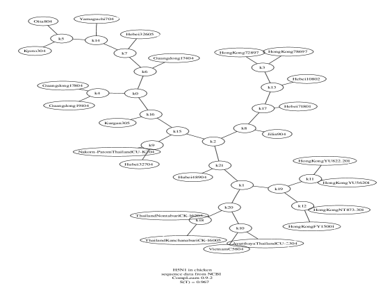
Figure 4: Set of 24 Chicken Examples of H5N1 Virii. $S(T)=0.967$.

In Figure 4 we display classification of bird-flu virii of the type H5N1 that have been found in different geographic locations in chicken. Data downloaded from the National Center for Biotechnology Information (NCBI), National Library of Medicine, National Institutes of Health (NIH).

4 Google-Based Similarity

To make computers more intelligent one would like to represent meaning in computer-digestable form. Long-term and labor-intensive efforts like the Cyc project [23] and the WordNet project [36] try to establish semantic relations between common objects, or, more precisely, names for those objects. The idea is to create a semantic web of such vast proportions that rudimentary intelligence and knowledge about the real world spontaneously emerges. This comes at the great cost of designing structures capable of manipulating knowledge, and entering high quality contents in these structures by knowledgeable human experts. While the efforts are long-running and large scale, the overall information entered is minute compared to what is available on the world-wide-web.

The rise of the world-wide-web has enticed millions of users to type in trillions of characters to create billions of web pages of on average low quality contents. The sheer mass of the information available about almost every conceivable topic makes it likely that extremes will cancel and the majority or average is meaningful in a low-quality approximate sense. We devise a general method to tap the amorphous low-grade knowledge available for free on the world-wide-web, typed in by local users aiming at personal gratification of diverse objectives, and yet globally achieving what is effectively the largest semantic electronic database in the world. Moreover, this database is available for all by using any search engine that can return aggregate page-count estimates like Google for a large range of search-queries.

The crucial point about the NCD method above is that the method analyzes the objects themselves. This precludes comparison of abstract notions or other objects that don’t lend themselves to direct analysis, like emotions, colors, Socrates, Plato, Mike Bonanno and Albert Einstein. While the previous NCD method that compares the objects themselves using (10) is particularly suited to obtain knowledge about the similarity of objects themselves, irrespective of common beliefs about such similarities, we now develop a method that uses only the name of an object and obtains knowledge about the similarity of objects by tapping available information generated by multitudes of web users. The new method is useful to extract knowledge from a given corpus of knowledge, in this case the Google database, but not to obtain true facts that are not common knowledge in that database. For example, common viewpoints on the creation myths in different religions may be extracted by the Googling method, but contentious questions of fact concerning the phylogeny of species can be better approached by using the genomes of these species, rather than by opinion.

Googling for Knowledge: Let us start with simple intuitive justification (not to be mistaken for a substitute of the underlying mathematics) of the approach we propose in [13]. While the theory we propose is rather intricate, the resulting method is simple enough. We give an example: At the time of doing the experiment, a Google search for “horse”, returned 46,700,000 hits. The number of hits for the search term “rider” was 12,200,000. Searching for the pages where both “horse” and “rider” occur gave 2,630,000 hits, and Google indexed 8,058,044,651 web pages. Using these numbers in the main formula (13) we derive below, with $N=8,058,044,651$, this yields a Normalized Google Distance between the terms “horse” and “rider” as follows:

$$\textsc{NGD}(horse,rider)\approx 0.443.$$

In the sequel of the paper we argue that the NGD is a normed semantic distance between the terms in question, usually in between 0 (identical) and 1 (unrelated), in the cognitive space invoked by the usage of the terms on the world-wide-web as filtered by Google. Because of the vastness and diversity of the web this may be taken as related to the current objective meaning of the terms in society. We did the same calculation when Google indexed only one-half of the current number of pages: 4,285,199,774. It is instructive that the probabilities of the used search terms didn’t change significantly over this doubling of pages, with number of hits for “horse” equal 23,700,000, for “rider” equal 6,270,000, and for “horse, rider” equal to 1,180,000. The $\textsc{NGD}(horse,rider)$ we computed in that situation was $\approx 0.460$. This is in line with our contention that the relative frequencies of web pages containing search terms gives objective information about the semantic relations between the search terms. If this is the case, then the Google probabilities of search terms and the computed NGD ’s should stabilize (become scale invariant) with a growing Google database.

Related Work: There is a great deal of work in both cognitive psychology [22], linguistics, and computer science, about using word (phrases) frequencies in text corpora to develop measures for word similarity or word association, partially surveyed in [37, 38], going back to at least [24]. One of the most successful is Latent Semantic Analysis (LSA) [22] that has been applied in various forms in a great number of applications. As with LSA, many other previous approaches of extracting meaning from text documents are based on text corpora that are many order of magnitudes smaller, using complex mathematical techniques like singular value decomposition and dimensionality reduction, and that are in local storage, and on assumptions that are more restricted, than what we propose. In contrast, [41, 8, 1] and the many references cited there, use the web and Google counts to identify lexico-syntactic patterns or other data. Again, the theory, aim, feature analysis, and execution are different from ours, and cannot meaningfully be compared. Essentially, our method below automatically extracts meaning relations between arbitrary objects from the web in a manner that is feature-free, up to the search-engine used, and computationally feasible. This seems to be a new direction altogether.

4.1 The Google Distribution

Let the set of singleton Google search terms be denoted by ${\cal S}$. In the sequel we use both singleton search terms and doubleton search terms $\{\{x,y\}:x,y\in{\cal S}\}$. Let the set of web pages indexed (possible of being returned) by Google be $\Omega$. The cardinality of $\Omega$ is denoted by $M=|\Omega|$, and at the time of this writing $8\cdot 10^{9}\leq M\leq 9\cdot 10^{9}$ (and presumably greater by the time of reading this). Assume that a priori all web pages are equi-probable, with the probability of being returned by Google being $1/M$. A subset of $\Omega$ is called an event. Every search term $x$ usable by Google defines a singleton Google event ${\bf x}\subseteq\Omega$ of web pages that contain an occurrence of $x$ and are returned by Google if we do a search for $x$. Let $L:\Omega\rightarrow[0,1]$ be the uniform mass probability function. The probability of such an event ${\bf x}$ is $L({\bf x})=|{\bf x}|/M$. Similarly, the doubleton Google event ${\bf x}\bigcap{\bf y}\subseteq\Omega$ is the set of web pages returned by Google if we do a search for pages containing both search term $x$ and search term $y$. The probability of this event is $L({\bf x}\bigcap{\bf y})=|{\bf x}\bigcap{\bf y}|/M$. We can also define the other Boolean combinations: $\neg{\bf x}=\Omega\backslash{\bf x}$ and ${\bf x}\bigcup{\bf y}=\neg(\neg{\bf x}\bigcap\neg{\bf y})$, each such event having a probability equal to its cardinality divided by $M$. If ${\bf e}$ is an event obtained from the basic events ${\bf x},{\bf y},\ldots$, corresponding to basic search terms $x,y,\ldots$, by finitely many applications of the Boolean operations, then the probability $L({\bf e})=|{\bf e}|/M$. Google events capture in a particular sense all background knowledge about the search terms concerned available (to Google) on the web. The Google event ${\bf x}$, consisting of the set of all web pages containing one or more occurrences of the search term $x$, thus embodies, in every possible sense, all direct context in which $x$ occurs on the web.

Remark 4

It is of course possible that parts of this direct contextual material link to other web pages in which $x$ does not occur and thereby supply additional context. In our approach this indirect context is ignored. Nonetheless, indirect context may be important and future refinements of the method may take it into account.

The event ${\bf x}$ consists of all possible direct knowledge on the web regarding $x$. Therefore, it is natural to consider code words for those events as coding this background knowledge. However, we cannot use the probability of the events directly to determine a prefix code, or, rather the underlying information content implied by the probability. The reason is that the events overlap and hence the summed probability exceeds 1. By the Kraft inequality, see for example [27], this prevents a corresponding set of code-word lengths. The solution is to normalize: We use the probability of the Google events to define a probability mass function over the set $\{\{x,y\}:x,y\in{\cal S}\}$ of Google search terms, both singleton and doubleton terms. There are $|{\cal S}|$ singleton terms, and ${|{\cal S}|\choose 2}$ doubletons consisting of a pair of non-identical terms. Define

$$N=\sum_{\{x,y\}\subseteq{\cal S}}|{\bf x}\bigcap{\bf y}|,$$

counting each singleton set and each doubleton set (by definition unordered) once in the summation. Note that this means that for every pair $\{x,y\}\subseteq{\cal S}$, with $x\neq y$, the web pages $z\in{\bf x}\bigcap{\bf y}$ are counted three times: once in ${\bf x}={\bf x}\bigcap{\bf x}$, once in ${\bf y}={\bf y}\bigcap{\bf y}$, and once in ${\bf x}\bigcap{\bf y}$. Since every web page that is indexed by Google contains at least one occurrence of a search term, we have $N\geq M$. On the other hand, web pages contain on average not more than a certain constant $\alpha$ search terms. Therefore, $N\leq\alpha M$. Define

$$g(x)=g(x,x),\;\;g(x,y)=L({\bf x}\bigcap{\bf y})M/N=|{\bf x}\bigcap{\bf y}|/N.$$ (11)

Then, $\sum_{\{x,y\}\subseteq{\cal S}}g(x,y)=1$. This $g$-distribution changes over time, and between different samplings from the distribution. But let us imagine that $g$ holds in the sense of an instantaneous snapshot. The real situation will be an approximation of this. Given the Google machinery, these are absolute probabilities which allow us to define the associated prefix code-word lengths (information contents) for both the singletons and the doubletons. The Google code $G$ is defined by

$$G(x)=G(x,x),\;\;G(x,y)=\log 1/g(x,y).$$ (12)

In contrast to strings $x$ where the complexity $C(x)$ represents the length of the compressed version of $x$ using compressor $C$, for a search term $x$ (just the name for an object rather than the object itself), the Google code of length $G(x)$ represents the shortest expected prefix-code word length of the associated Google event ${\bf x}$. The expectation is taken over the Google distribution $p$. In this sense we can use the Google distribution as a compressor for Google “meaning” associated with the search terms. The associated NCD , now called the normalized Google distance ( NGD ) is then defined by (13), and can be rewritten as the right-hand expression:

$$\textsc{NGD}(x,y)=\frac{G(x,y)-\min(G(x),G(y))}{\max(G(x),G(y))}=\frac{\max\{\log f(x),\log f(y)\}-\log f(x,y)}{\log N-\min\{\log f(x),\log f(y)\}},$$ (13)

where $f(x)$ denotes the number of pages containing $x$, and $f(x,y)$ denotes the number of pages containing both $x$ and $y$, as reported by Google. This NGD is an approximation to the NID of (7) using the prefix code-word lengths (Google code) generated by the Google distribution as defining a compressor approximating the length of the Kolmogorov code, using the background knowledge on the web as viewed by Google as conditional information. In practice, use the page counts returned by Google for the frequencies, and we have to choose $N$. From the right-hand side term in (13) it is apparent that by increasing $N$ we decrease the NGD , everything gets closer together, and by decreasing $N$ we increase the NGD , everything gets further apart. Our experiments suggest that every reasonable ($M$ or a value greater than any $f(x)$) value can be used as normalizing factor $N$, and our results seem in general insensitive to this choice. In our software, this parameter $N$ can be adjusted as appropriate, and we often use $M$ for $N$.

Universality of NGD: In the full paper [13] we analyze the mathematical properties of NGD , and prove the universality of the Google distribution among web author based distributions, as well as the universality of the NGD with respect to the family of the individual web author’s NGD ’s, that is, their individual semantics relations, (with high probability)—not included here for space reasons.

5 Applications

5.1 Colors and Numbers

The objects to be clustered are search terms consisting of the names of colors, numbers, and some tricky words. The program automatically organized the colors towards one side of the tree and the numbers towards the other, Figure 5.

Figure 5: Colors and numbers arranged into a tree using NGD .

It arranges the terms which have as only meaning a color or a number, and nothing else, on the farthest reach of the color side and the number side, respectively. It puts the more general terms black and white, and zero, one, and two, towards the center, thus indicating their more ambiguous interpretation. Also, things which were not exactly colors or numbers are also put towards the center, like the word “small”. We may consider this an example of automatic ontology creation. As far as the authors know there do not exist other experiments that create this type of semantic meaning from nothing (that is, automatically from the web using Google). Thus, there is no baseline to compare against; rather the current experiment can be a baseline to evaluate the behavior of future systems.

5.2 Names of Literature

Another example is English novelists. The authors and texts used are:

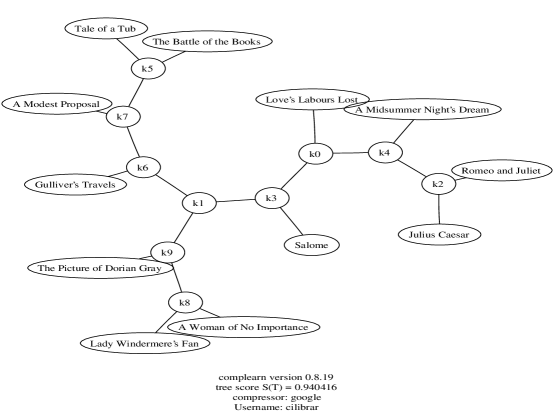
Figure 6: Hierarchical clustering of authors. $S(T)=0.940$.

William Shakespeare: A Midsummer Night’s Dream; Julius Caesar; Love’s Labours Lost; Romeo and Juliet .

Jonathan Swift: The Battle of the Books; Gulliver’s Travels; Tale of a Tub; A Modest Proposal;

Oscar Wilde: Lady Windermere’s Fan; A Woman of No Importance; Salome; The Picture of Dorian Gray.

As search terms we used only the names of texts, without the authors. The clustering is given in Figure 6; it automatically has put the books by the same authors together. The $S(T)$ value in Figure 6 gives the fidelity of the tree as a representation of the pairwise distances in the NGD matrix (1 is perfect and 0 is as bad as possible. For details see [7, 12]). The question arises why we should expect this. Are names of artistic objects so distinct? (Yes. The point also being that the distances from every single object to all other objects are involved. The tree takes this global aspect into account and therefore disambiguates other meanings of the objects to retain the meaning that is relevant for this collection.) Is the distinguishing feature subject matter or title style? (In these experiments with objects belonging to the cultural heritage it is clearly a subject matter. To stress the point we used “Julius Caesar” of Shakespeare. This term occurs on the web overwhelmingly in other contexts and styles. Yet the collection of the other objects used, and the semantic distance towards those objects, determined the meaning of “Julius Caesar” in this experiment.) Does the system gets confused if we add more artists? (Representing the NGD matrix in bifurcating trees without distortion becomes more difficult for, say, more than 25 objects. See [12].) What about other subjects, like music, sculpture? (Presumably, the system will be more trustworthy if the subjects are more common on the web.) These experiments are representative for those we have performed with the current software. For a plethora of other examples, or to test your own, see the Demo page of [7].

5.3 Systematic Comparison with WordNet Semantics

WordNet [36] is a semantic concordance of English. It focusses on the meaning of words by dividing them into categories. We use this as follows. A category we want to learn, the concept, is termed, say, “electrical”, and represents anything that may pertain to electronics. The negative examples are constituted by simply everything else. This category represents a typical expansion of a node in the WordNet hierarchy. In an experiment we ran, the accuracy on the test set is 100%: It turns out that “electrical terms” are unambiguous and easy to learn and classify by our method. The information in the WordNet database is entered over the decades by human experts and is precise. The database is an academic venture and is publicly accessible. Hence it is a good baseline against which to judge the accuracy of our method in an indirect manner. While we cannot directly compare the semantic distance, the NGD , between objects, we can indirectly judge how accurate it is by using it as basis for a learning algorithm. In particular, we investigated how well semantic categories as learned using the NGD – SVM approach agree with the corresponding WordNet categories. For details about the structure of WordNet we refer to the official WordNet documentation available online. We considered 100 randomly selected semantic categories from the WordNet database. For each category we executed the following sequence. First, the SVM is trained on 50 labeled training samples. The positive examples are randomly drawn from the WordNet database in the category in question. The negative examples are randomly drwan from a dictionary. While the latter examples may be false negatives, we consider the probability negligible. Per experiment we used a total of six anchors, three of which are randomly drawn from the WordNet database category in question, and three of which are drawn from the dictionary. Subsequently, every example is converted to 6-dimensional vectors using NGD . The $i$th entry of the vector is the NGD between the $i$th anchor and the example concerned ($1\leq i\leq 6$). The SVM is trained on the resulting labeled vectors. The kernel-width and error-cost parameters are automatically determined using five-fold cross validation. Finally, testing of how well the SVM has learned the classifier is performed using 20 new examples in a balanced ensemble of positive and negative examples obtained in the same way, and converted to 6-dimensional vectors in the same manner, as the training examples. This results in an accuracy score of correctly classified test examples. We ran 100 experiments. The actual data are available at [10].

Figure 7: Histogram of accuracies over 100 trials of WordNet experiment.

A histogram of agreement accuracies is shown in Figure 7. On average, our method turns out to agree well with the WordNet semantic concordance made by human experts. The mean of the accuracies of agreements is 0.8725. The variance is $\approx 0.01367$, which gives a standard deviation of $\approx 0.1169$. Thus, it is rare to find agreement less than 75%. The total number of Google searches involved in this randomized automatic trial is upper bounded by $100\times 70\times 6\times 3=126,000$. A considerable savings resulted from the fact that we can re-use certain google counts. For every new term, in computing its 6-dimensional vector, the NGD computed with respect to the six anchors requires the counts for the anchors which needs to be computed only once for each experiment, the count of the new term which can be computed once, and the count of the joint occurrence of the new term and each of the six anchors, which has to be computed in each case. Altogether, this gives a total of $6+70+70\times 6=496$ for every experiment, so $49,600$ google searches for the entire trial.

References

- [1] J.P. Bagrow, D. ben-Avraham, On the Google-fame of scientists and other populations, AIP Conference Proceedings 779:1(2005), 81–89.
- [2] D. Benedetto, E. Caglioti, and V. Loreto, Language trees and zipping, Phys. Review Lett., 88:4(2002) 048702.
- [3] C.H. Bennett, P. Gács, M. Li, P.M.B. Vitányi, W. Zurek, Information Distance, IEEE Trans. Information Theory, 44:4(1998), 1407–1423. (Conference version: “Thermodynamics of Computation and Information Distance,” In: Proc. 25th ACM Symp. Theory of Comput., 1993, 21-30.)
- [4] C.H. Bennett, M. Li, B. Ma, Chain letters and evolutionary histories, Scientific American, June 2003, 76–81.
- [5] C.J.C. Burges. A tutorial on support vector machines for pattern recognition, Data Mining and Knowledge Discovery, 2:2(1998),121–167.
- [6] X. Chen, B. Francia, M. Li, B. McKinnon, A. Seker, Shared information and program plagiarism detection, IEEE Trans. Inform. Th., 50:7(2004), 1545–1551.
- [7] R. Cilibrasi, The CompLearn Toolkit, CWI, 2003–, http://www.complearn.org/
- [8] P. Cimiano, S. Staab, Learning by Googling, SIGKDD Explorations, 6:2(2004), 24–33.
- [9] W. Chai and B. Vercoe. Folk music classification using hidden Markov models. Proc. of International Conference on Artificial Intelligence, 2001.
- [10] R. Cilibrasi, P. Vitanyi, Automatic Meaning Discovery Using Google: 100 Experiments in Learning WordNet Categories, 2004, http://www.cwi.nl/cilibrar/googlepaper/appendix.pdf
- [11] R. Cilibrasi, R. de Wolf, P. Vitanyi. Algorithmic clustering of music based on string compression, Computer Music J., 28:4(2004), 49-67. Web version: http://xxx.lanl.gov/abs/cs.SD/0303025
- [12] R. Cilibrasi, P.M.B. Vitanyi, Clustering by compression, IEEE Trans. Information Theory, 51:4(2005), 1523- 1545. Web version: http://xxx.lanl.gov/abs/cs.CV/0312044
- [13] R. Cilibrasi, P. Vitanyi, Automatic meaning discovery using Google, Manuscript, CWI, 2004; http://arxiv.org/abs/cs.CL/0412098
- [14] R. Cilibrasi, P.M.B. Vitanyi, A New Quartet Tree Heuristic for Hierarchical Clustering, EU-PASCAL Statistics and Optimization of Clustering Workshop, 5-6 Juli 2005, London, UK. http://homepages.cwi.nl/ paulv/papers/quartet.pdf
- [15] R. Dannenberg, B. Thom, and D. Watson. A machine learning approach to musical style recognition, Proc. International Computer Music Conference, pp. 344-347, 1997.
- [16] R. Duda, P. Hart, D. Stork. Pattern Classification, John Wiley and Sons, 2001.
- [17] The basics of Google search, http://www.google.com/help/basics.html.
- [18] M. Grimaldi, A. Kokaram, and P. Cunningham. Classifying music by genre using the wavelet packet transform and a round-robin ensemble. Technical report TCD-CS-2002-64, Trinity College Dublin, 2002. http://www.cs.tcd.ie/publications/tech-reports/reports.02/TCD-CS-2002-64.pdf
- [19] E. Keogh, S. Lonardi, and C.A. Rtanamahatana, Toward parameter-free data mining, In: Proc. 10th ACM SIGKDD Intn’l Conf. Knowledge Discovery and Data Mining, Seattle, Washington, USA, August 22—25, 2004, 206–215.
- [20] A.N. Kolmogorov. Three approaches to the quantitative definition of information, Problems Inform. Transmission, 1:1(1965), 1–7.
- [21] A.N. Kolmogorov. Combinatorial foundations of information theory and the calculus of probabilities, Russian Math. Surveys, 38:4(1983), 29–40.
- [22] T. Landauer and S. Dumais, A solution to Plato’s problem: The latent semantic analysis theory of acquisition, induction and representation of knowledge, Psychol. Rev., 104(1997), 211–240.
- [23] D. B. Lenat. Cyc: A large-scale investment in knowledge infrastructure, Comm. ACM, 38:11(1995),33–38.
- [24] M.E. Lesk, Word-word associations in document retrieval systems, American Documentation, 20:1(1969), 27–38.
- [25] M. Li and P.M.B. Vitányi, Theory of thermodynamics of computation, Proc. IEEE Physics of Computation Workshop, Dallas (Texas), Oct. 4-6, 1992, pp. 42-46. A full version (basically the here relevant part of [26]) appeared in the Preliminary Proceedings handed out at the Workshop.
- [26] M. Li and P.M.B. Vitányi, Reversibility and adiabatic computation: trading time and space for energy, Proc. Royal Society of London, Series A, 452(1996), 769-789.
- [27] M. Li and P.M.B. Vitányi, An Introduction to Kolmogorov Complexity and its Applications, Springer-Verlag, New York, 2nd Edition, 1997.
- [28] X. Chen, S. Kwong, M. Li. A compression algorithm for DNA sequences based on approximate matching. In: Proc. 10th Workshop on Genome Informatics (GIW), number 10 in the Genome Informatics Series, Tokyo, December 14-15 1999. Also in Proc. 4th ACM RECOMB, 2000, p. 107.
- [29] M. Li, J.H. Badger, X. Chen, S. Kwong, P. Kearney, and H. Zhang, An information-based sequence distance and its application to whole mitochondrial genome phylogeny, Bioinformatics, 17:2(2001), 149–154.
- [30] M. Li and P.M.B. Vitányi, Algorithmic Complexity, pp. 376–382 in: International Encyclopedia of the Social & Behavioral Sciences, N.J. Smelser and P.B. Baltes, Eds., Pergamon, Oxford, 2001/2002.
- [31] M. Li, X. Chen, X. Li, B. Ma, P. Vitanyi. The similarity metric, IEEE Trans. Information Theory, 50:12(2004), 3250- 3264. (Conference version in: Proc. 14th ACM-SIAM Symposium on Discrete Algorithms, Baltimore, USA, 2003, pp 863-872.) Web version: http://xxx.lanl.gov/abs/cs.CC/0111054
- [32] M. Li, P. M. B. Vitanyi. An Introduction to Kolmogorov Complexity and Its Applications, 2nd Ed., Springer-Verlag, New York, 1997.
- [33] S. L. Reed, D. B. Lenat. Mapping ontologies into cyc. Proc. AAAI Conference 2002 Workshop on Ontologies for the Semantic Web, Edmonton, Canada. http://citeseer.nj.nec.com/509238.html
-
[34]
P. Scott.
Music classification using neural networks, 2001.
http://www.stanford.edu/class/ee373a/musicclassification.pdf - [35] K. Strimmer, A. von Haeseler. “Quartet puzzling: A quartet maximum likelihood method for reconstructing tree topologies”, Mol Biol Evol, 1996, 13 pp. 964-969.
-
[36]
G.A. Miller et.al, WordNet,
A Lexical Database for the English Language,
Cognitive Science Lab, Princeton University.
http://www.cogsci.princeton.edu/wn - [37] E. Terra and C. L. A. Clarke. Frequency Estimates for Statistical Word Similarity Measures. HLT/NAACL 2003, Edmonton, Alberta, May 2003. 37/162
- [38] P.-N. Tan, V. Kumar, J. Srivastava, Selecting the right interestingness measure for associating patterns. Proc. ACM-SIGKDD Conf. Knowledge Discovery and Data Mining, 2002, 491–502.
- [39] G. Tzanetakis and P. Cook, Music genre classification of audio signals, IEEE Transactions on Speech and Audio Processing, 10(5):293–302, 2002.
- [40] S. Wehner, Analyzing network traffic and worms using compression, http://arxiv.org/abs/cs.CR/0504045
- [41] Corpus collosal: How well does the world wide web represent human language? The Economist, January 20, 2005. http://www.economist.com/science/displayStory.cfm?story_id=3576374