Incremental Redundancy Cooperative Coding for Wireless Networks:
Cooperative Diversity, Coding, and Transmission Energy Gain

Abstract

We study an incremental redundancy (IR) cooperative coding scheme for wireless networks. To exploit the distributed spatial diversity benefit we propose a cluster-based collaborating strategy for a quasi-static Rayleigh fading channel model. Our scheme allows for enhancing the reliability performance of a direct communication over a single hop. The collaborative cluster consists of $M-1$ nodes between the sender and the destination. The transmitted message is encoded using a mother code which is partitioned into $M$ blocks each assigned to one of $M$ transmission slots. In the first slot, the sender broadcasts its information by transmitting the first block, and its helpers attempt to relay this message. In the remaining slots, each of left-over $M-1$ blocks is sent either through a helper which has successfully decoded the message or directly by the sender where a dynamic schedule is based on the ACK-based feedback from the cluster. By employing powerful good codes including turbo, low-density parity-check, and repeat-accumulate codes, our approach illustrates the benefit of collaboration through not only a cooperation diversity gain but also a coding advantage. The basis of our error rate performance analysis is the threshold behavior of good codes. We derive a new simple code threshold for the Bhattacharyya distance based on the modified Shulman-Feder bound and the relationship between the Bhattacharyya parameter and the channel capacity for an arbitrary binary-input symmetric-output memoryless channel. The study of the diversity and the coding gain of the proposed scheme is based on this new threshold. An average frame-error rate (FER) upper bound and its asymptotic (in SNR) version are derived as a function of the average fading channel SNRs and the code threshold. Based on the asymptotic bound, we investigate both the diversity, the coding, and the transmission energy gain in the high and moderate SNR regimes for three different scenarios: transmitter clustering, receiver clustering, and cluster hopping. Furthermore, given a geometric distance profile of the network, we have observed that the energy saving of the IR cooperative coding scheme is universal for all good code families.

I Introduction

To overcome fading, wireless networks employ various diversity techniques, e.g., channel interleavers, multiple antennas, frequency hopping, etc. In [1], Sendonaris, Erkip, and Aazhang have proposed the so-called user-cooperation diversity where users partner in sharing their antennas and other resources to create a virtual array through distributed transmission and signal processing. Only limited time and frequency diversity is available when the transmitted signal experiences a quasi-static frequency-flat fading and the receiver has a strict decoding delay constraint (as in speech and video transmission). In this case, introducing spatial diversity through cooperation is especially beneficial.

Motivated by the increasing importance of cooperative communication in wireless networks, a large of valuable work has gone into designing the collaborative protocols, assessing the information-theoretic limits, and evaluating the cooperative benefit in the past few years. An information-theoretic analysis of several cooperative protocols has been reported in [2, 3] based on repetition-coding and space-time-coding. In an independent, relevant work [4], the authors have studied the outage probability and the asymptotic error probability performance calculations of a two-user incremental redundancy coding scheme based on Gaussian codebooks. An practical coding strategy for two-user collaborating transmission based on rate compatible punctured convolutional codes has been considered in [5, 6]. Cooperation schemes employing distributed turbo codes have been studied in [7, 8, 9], where [8] has focused on the asymptotic error performance analysis.

In this paper, we study an incremental redundancy (IR) cooperative coding scheme for a multiple-helper wireless network. To exploit the spatial diversity benefit we propose a cluster-based collaborating strategy for a quasi-static Rayleigh fading channel model and based on a network geometric distance profile [10]. The cluster-based collaborating strategy enhances the reliability performance of a direct communication over a single hop. A collaborative cluster consists of $M-1$ nodes assisting the sender in a two-hop strategy. The transmitted message is encoded using a mother code which is partitioned into $M$ blocks each assigned to one of $M$ transmission slots. In the first slot, the sender broadcasts own information by transmitting the first block, and its helpers attempt to decode the message. In the remaining slots, each of the left-over $M-1$ blocks is sent either through a helper which has successfully decoded the message or directly by the sender based on an acknowledgement (ACK) driven a dynamic schedule. By employing the powerful good codes [11, 12], e.g., turbo, low-density parity-check (LDPC), and repeat-accumulate (RA) codes, whose performance is characterized by a threshold behavior, our approach illustrates the benefit of collaboration through not only a cooperation diversity but also a coding advantage.

To investigate benefits of the proposed IR cooperative coding scheme, we evaluate its frame error rate (FER) performance for a quasi-static frequency-flat Rayleigh fading channel. The basis of our error rate performance analysis is the so-called code threshold of a good code ensemble. Our focus is on the code threshold for which the maximum likelihood (ML) decoding word error probability vanishes whenever the channel quality is above the threshold. In fact, we propose a new Bhattacharyya distance simple code threshold for parallel channel transmissions based on the modified Shulman-Feder reliable channel region [13, 14, 15] and the relationship between the Bhattacharyya parameter and the channel capacity of an arbitrary binary-input symmetric-output memoryless (BISOM) channel [16]. The derived threshold characterizes a reliable communication condition for parallel channel transmissions with a single constraint in terms of the average Bhattacharyya parameter. Compared with the union Bhattacharyya (UB) code threshold introduced in [17], the new code threshold is almost tighter $1~{}dB$ for an example turbo code transmitted over a binary-input AWGN (BI-AWGN) channel, as illustrated in Example 1.

Next, based on the simple code threshold and the outage concept, we derive a FER upper-bound which predicts well the fading channel simulation results for the proposed cooperative coding scheme. Compared with the result in [6] (and the block-fading channel FER bound in [18]), the derived FER bound is a function of the single code threshold parameter instead of a family of weight enumerators. Hence, this simple FER bound is not only easy to compute but is also insightful in that it allows for a large SNR asymptotic analysis of the cooperation scheme. In this paper, closed-form asymptotic FER upper-bounds are obtained for three different scenarios: transmitter clustering, receiver clustering, and cluster hopping. These bounds allow for illustrating cooperative diversity and coding gains in the high SNR regime. Finally, we express FER bounds in terms of the distance profile and investigate cooperation benefits in terms of the energy efficiency gain for different collaborative cluster sizes and normalized cluster distances.

The paper is organized as follows. We describe the system model in Sec. II. We study the threshold behavior of good code ensembles over BISOM channels in Sec. III. An IR cooperative coding scheme is introduced in Sec. IV. We derive an upper bound on the scheme FER in Sec. V, and its asymptotic versions for different cooperation scenarios in Sec. VI. Simulation results and the collaborative cluster design are discussed in Sec. VII. Finally, we summarize our results in Sec. VIII.

II System Model

In this section, we introduce a collaborative cluster and describe a fading channel model based on the geometric distance profile of the network.

II-A Collaborative Cluster

As shown in Fig. 1, we consider a single sender-destination pair and several intermediate nodes. A group of $M-1$ nodes forms a collaborative cluster $\mathcal{S}$ which assists the sender in a two-hop scheme. The sender serves as the regional broadcast node, and each cluster member, termed helper, attempts to relay the package to the destination.

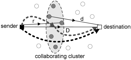
Figure 1: Cooperative routing in wireless network with a geometric distance profile

For notational convenience, let Node $0$ denote the sender, Node $m$, for $m=1,\dots,M-1$, denote a helper, and Node $M$ denote the destination.

Remark 1

The proposed cluster-based collaborating strategy can be embedded into an existing noncooperative route. For example, the routing metric most commonly used in existing ad hoc routing protocols is the minimum hop-count, which results in a long distance traveled by each hop [19]. Hence, there may exist several intermediate nodes between the (hop) sender and the (hop) destination for each non-cooperation hop. This is one of the motivations for the IR cooperative coding scheme proposed in this paper, namely, the cooperative scheme is a supplement to current routing algorithms for overcoming the “dynamic” deep fade.

II-B Channel Model

We consider the quasi-static frequency-flat Rayleigh fading channel model [20] where the fading coefficient is random but invariant during the transmission interval $T$. The discrete-time channel model is

$$y_{i,j} =d_{i,j}^{-L/2}\,a_{i,j}\,x_{i}+z_{i,j}~{}~{}\text{for}~{}i\in\{0,\dots,M-1\}~{}\text{and}~{}j\in\{1,\dots,M\}$$ (1)

where $x_{i}$ is the signal transmitted by Node $i$, $L$ is the path loss exponent, $d_{i,j}$, $a_{i,j}$, and $z_{i,j}$ are the distance, fading coefficient, and background noise between Nodes $i$, $j$, respectively, and $y_{i,j}$ is the signal at Node $j$ received from Node $i$. We will focus on the transmitted signal alphabet is binary, i.e., $x_{i}\in\bigl{\{}+\sqrt{E},-\sqrt{E}\bigr{\}}$, where $E$ is the transmitted symbol energy which is identical for all cluster nodes and the sender, and the symbol “$+\sqrt{E}$” (and “$-\sqrt{E}$”) represents the coded symbol “$0$” (and “$1$”). We assume that $z_{i,j}$ is modeled as the mutually independent additive Gaussian noise ${\mathcal{N}}(0,1/2)$, and $\nu_{i,j}=|a_{i,j}|^{2}$ is the exponentially distributed “channel power” with mean $1$. Then, the average and instantaneous SNRs of the signal at Node $j$ received from Node $i$ can respectively be expressed as

$${\sf SNR}_{i,j}\triangleq E\cdot d_{i,j}^{-L},~{}~{}\text{and}~{}~{}\theta_{i,j}\triangleq\nu_{i,j}\cdot{\sf SNR}_{i,j}.$$

We further assume that decoding is done with the knowledge of the fading coefficients. Note that, for a given fading coefficient $a_{i,j}$, the channel (1) is a BI-AWGN channel. This motivates us to study the error performance of binary good code ensembles transmitted over BISOM channels in the next section.

III Threshold Based Performance Analysis for BISOM channels

In this section, we introduce the notation and the preliminary material on BISOM channel measures and the weight spectrum of code ensembles. Next, we study the threshold behavior of good code ensembles and derive a new simple code threshold for parallel channel transmissions. Results given in this section are used as the foundation for the error performance analysis of the IR cooperative coding scheme.

III-A Channel Capacity and Bhattacharyya Parameter of BISOM Channels

Here, we consider a binary input memoryless channel with the output alphabet $\mathcal{Y}$ and transition probabilities $p(y|0)$ and $p(y|1)$, $y\in\mathcal{Y}$. We say that the channel is symmetric if $p(y|0)=p(-y|1)$. We first study the channel capacity and the Bhattacharyya parameter for BISOM channels. The Bhattacharyya parameter is widely used to characterize the “noisiness” of the channel (e.g., see [17, 15]). The capacity of a BISOM channel is achieved by the uniform input distribution and can be expressed in terms of $p(y|0)$ as follows

$$C =\frac{1}{2}\Biggl{[}\sum_{y\in{\mathcal{Y}}}p(y|0)\log_{2}\frac{p(y|0)}{p(y)}+\sum_{y\in{\mathcal{Y}}}p(y|1)\log_{2}\frac{p(y|1)}{p(y)}\Biggr{]}$$

$$={\sf E}\left[\log_{2}\frac{p(Y|0)}{p(Y)}\Biggl{|}\,0\right]$$

$$=1-{\sf E}\left[\log_{2}\frac{p(Y|0)+p(-Y|0)}{p(Y|0)}\Biggl{|}\,0\right].$$ (2)

Similarly, the Bhattacharyya parameter $\gamma$ is

$$\gamma =\sum_{y\in{\mathcal{Y}}}\sqrt{p(y|0)p(y|1)}={\sf E}\left[\sqrt{\frac{p(-Y|0)}{p(Y|0)}}\Biggl{|}\,0\right].$$ (3)

We also consider the cutoff rate for the BISOM channel,

$$R_{0}\triangleq 1-\log_{2}(1+\gamma).$$ (4)

Now, we establish a general relationship among these three information-theoretic quantities in the following lemma.

Lemma 1

Let $B\triangleq 1-\gamma$ denote the Bhattacharyya rate. For a BISOM channel with a transition probability $p(y|0)$, the channel capacity, the Bhattacharyya rate, and the cutoff rate satisfy

$$C\geq B\geq R_{0}.$$ (5)

Proof.

The proof in Appendix -C follows the Jensen’s inequality. ∎

In Lemma 1, we propose a new channel quality measure called Bhattacharyya rate which is between the channel capacity and the cutoff rate.

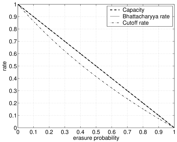
a. BEC

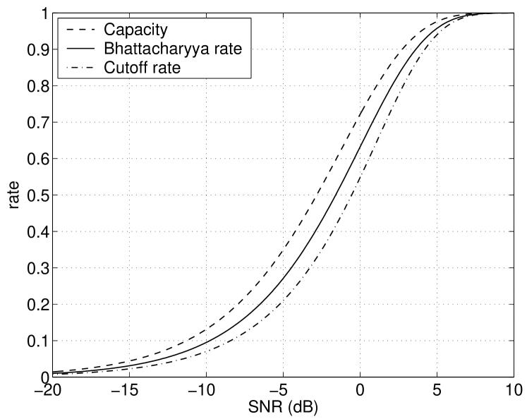
b. BI-AWGN channel

Figure 2: Capacity, Bhattacharyya rate, and cutoff rate for BECs and BI-AWGN channels

In particular, the Bhattacharyya rate is equal to the channel capacity for the case of the binary erasure channel (BEC). For the case of a BI-AWGN channel with the SNR $\lambda$,

$$C(\lambda) =1-\frac{1}{\sqrt{\pi}}\int_{-\infty}^{+\infty}e^{-(y-\sqrt{\lambda})^{2}}\log_{2}\bigl{(}1+e^{-4y\sqrt{\lambda}}\bigr{)}\,dy$$ (6)

$$B(\lambda) =1-e^{-\lambda}$$ (7)

$$R_{0}(\lambda) =1-\log_{2}(1+e^{-\lambda}).$$ (8)

Clearly, for a BI-AWGN channel, the numerical calculation of the Bhattacharyya rate is much easier than the computation of the channel capacity which requires integration form from $-\infty$ to $\infty$. The channel capacity, the Bhattacharyya rate, and the cutoff rate are illustrated in Fig. 2 for BECs and BI-AWGN channels.

III-B Weight Spectrum Properties of Good Code Ensembles

In this paper, we consider good binary linear code ensembles [11, 12] whose performance is characterized by a threshold behavior. The class of good codes includes turbo, LDPC, and RA codes, and some recent variations. Due to the outstanding performance of such random-like codes, we employ these in our IR cooperative coding scheme. In order to evaluate the error performance of the cooperation scheme, we study code thresholds based on the weight spectrum of code ensembles. The weight spectrum for various good code ensembles were studied in, e.g., [21, 17, 22, 23]. In this subsection, we briefly introduce some notation on weight spectra of binary linear code ensembles, review the UB code threshold proposed in [17], and describe a relationship between the UB code threshold and the code rate.

For a given binary linear code ensemble $[{\mathcal{C}}]$ of length $N$ and rate $R$, let $A^{[{\mathcal{C}}]}_{h}$ denote the average number of codewords of Hamming weight $h$, termed the average weight enumerator (AWE). Let $\delta\triangleq h/N$ denote the normalized Hamming weights, then the asymptotic normalized exponent of the weight spectrum with respect to the codeword length is defined as

$$r^{[{\mathcal{C}}]}(\delta)\triangleq\limsup_{N\rightarrow\infty}\frac{\ln A^{[{\mathcal{C}}]}_{h}}{N}$$ (9)

where the superscript $[{\mathcal{C}}]$ denotes a binary code ensemble. To simplify notation, hereafter, we drop the superscript $[{\mathcal{C}}]$ from code parameters, e.g., in $r^{[{\mathcal{C}}]}(\delta)$ and $A^{[{\mathcal{C}}]}_{h}$, when we do not specify a particular code ensemble. Now, the Shulman-Feder (SF) distance [13]

$$\xi\triangleq\sup_{0<\delta\leq 1}\bigl{[}r(\delta)-r^{[\mathcal{RB}]}(\delta)\bigr{]}\log_{2}e$$ (10)

measures the weight spectrum distance between the random binary code ensemble $[\mathcal{RB}]$ and the code ensemble $[{\mathcal{C}}]$, where

$$r^{[\mathcal{RB}]}(\delta)=H(\delta)-(1-R)\ln 2$$

is the asymptotic normalized exponent of the weight spectrum for the random binary code ensemble and

$$H(\delta)\triangleq-\delta\ln(\delta)-(1-\delta)\ln(1-\delta)$$

is the binary entropy function. Following [17], we define the UB code threshold of a code ensemble $[{\mathcal{C}}]$ as

$$c_{0}\triangleq\sup_{0<\delta\leq 1}\frac{r(\delta)}{\delta}.$$ (11)

In this paper, we consider a family of good code ensembles whose weight spectra satisfies the following condition:

1. For a given binary code ensemble $[{\mathcal{C}}]$, there exists a sequence of integers $D_{N}$($<N$) such that $D_{N}\rightarrow\infty$ and

   $$\lim_{N\rightarrow\infty}\sum_{h=1}^{D_{N}}A_{h}=0;$$ (12)

2. and the UB code threshold $c_{0}$ is finite.

Finally, we establish a relationship between the code rate $R$ and the threshold $c_{0}$ in the following lemma.

Lemma 2

For a good binary linear code ensemble $[{\mathcal{C}}]$ of rate $R$, the UB code threshold $c_{0}$ is lower bounded by the following function of $R$,

$$c_{0}\geq-\ln(1-R).$$ (13)

Proof.

We show the proof in Appendix -D. ∎

III-C Threshold Behavior of Good Codes for BISOM Channels

The basis of our analysis is the threshold behavior of good codes. Here, we first review the work in [17, 24], which has studied the error performance of good code ensembles (e.g., turbo codes) based on the UB code threshold $c_{0}$. Next, we introduce a tighter Bhattacharyya distance code threshold $c_{\star}$ (compared with $c_{0}$) under ML decoding. Based on the new threshold $c_{\star}$, we derive a coding theorem for good code ensembles whose transmission takes place over independent parallel channels.

III-C1 UB Code Threshold

In [17], Jin and McEliece have shown that, for a binary-input memoryless channel, if

$$\gamma<\exp(-c_{0}),$$ (14)

the average ML decoding word error probability approaches zero. Inequality (14) describes a reliable communication condition for the code ensemble $[{\mathcal{C}}]$ based on a single channel parameter $\gamma$ and a single code parameter $c_{0}$, where the Bhattacharyya parameter $\gamma$ represents the “noisiness” level of the channel and the UB code threshold $c_{0}$ characterizes weight spectrum properties of the code ensemble. This result is based on the classical union bound. Hence, the threshold $c_{0}$ is loose. Based on $c_{0}$ and the random assignment method (described below), we have studied this bound for parallel BISOM channels [24, 15].

III-C2 Simple Code Threshold

Following the approach in [14], for a given good code ensemble $[{\mathcal{C}}]$ of rate $R$, we partition the normalized Hamming weights $\delta$ into two disjoint subsets,

$$\Psi(P) \triangleq\{\delta:0<\delta\leq 0.5-P\text{ or }0.5+P<\delta\leq 1\}$$

$$\Psi^{c}(P) \triangleq\{\delta:0.5-P<\delta\leq 0.5+P\},\text{ for }P\in[0,\,0.5).$$

Next, we define a new Bhattacharyya distance code threshold by optimizing the weight partition parameter $P$ as follows

$$c_{\star}\triangleq\min_{0\leq P<0.5}\left\{c_{P}:~{}c_{P}\geq-\ln(1-R-\xi_{P})\right\}$$ (15)

where

$$c_{P}\triangleq\sup_{\delta\in\Psi(P)}\frac{r(\delta)}{\delta}$$ (16)

denotes the restriction UB code threshold corresponding to the weight subsets $\Psi(P)$, and

$$\xi_{P}\triangleq\left\{\begin{array}[]{ll}\displaystyle{\sup_{\delta\in\Psi^{c}(P)}\bigl{[}r(\delta)-r^{[\mathcal{RB}]}(\delta)\bigr{]}\log_{2}e},&P>0\\ 0,&P=0.\end{array}\right.$$ (19)

denotes the restriction SF distance corresponding to the weight subsets $\Psi^{c}(P)$. Note that, in the case $P=0$,

$$c_{P}=c_{0}\quad\text{and}\quad\xi_{P}=0.$$

Hence, Lemma 2 and (15) imply that the new code threshold $c_{\star}\leq c_{0}$.

Now, we consider the average error rate performance of a code ensemble $[{\mathcal{C}}]$ transmitted over $Q$ parallel channels. Following the random assignment approach [24], we assume that the bits of the transmitted codeword are randomly assigned to parallel channels so that each bit is transmitted over Channel $j$ with the a-prior probability $\tau_{j}$, where $\sum_{j=0}^{Q-1}\tau_{j}=1$ and $\tau_{j}>0$ for $j=0,\dots,Q-1$. We have the following parallel channel coding theorem for the code ensemble $[{\mathcal{C}}]$ based on $c_{\star}$.

Theorem 1

Let us consider a linear binary code ensemble $[{\mathcal{C}}]$ whose transmission takes place over $Q$ independent parallel BISOM channels. Assume that the bits of the transmitted codeword are randomly assigned to the channels with assignment rates $\{\tau_{0},\dots,\tau_{Q-1}\}$. Let

$$\bar{\gamma}\triangleq\sum_{j=0}^{Q-1}\tau_{j}\gamma_{j}$$ (20)

be the average Bhattacharyya parameter over $Q$ parallel channels, where $\gamma_{j}$ is Bhattacharyya parameter of Channel $j$, for $j=0,\dots,Q-1$. If

$$\bar{\gamma}<\exp(-c_{\star}),$$ (21)

then the average ML decoding word error probability $P_{W}(\bar{\gamma},N)\stackrel{{\scriptstyle N}}{{\longrightarrow}}0.$

Proof.

The proof is based on the relationship between the channel capacity and the Bhattacharyya rate in Lemma 1, the lower bound on the UB code threshold in Lemma 2, and the modified Shulman-Feder reliable channel region in Appendix -A (please also refer to [12] for details). We provide the proof of Theorem 1 in Appendix -E. ∎

In Theorem 1, the reliable communication condition (21) is a simple constraint in terms of the average Bhattacharyya parameter. The new code threshold allows for characterizing more complex coding schemes (e.g., communication over block-fading channel where the error performance requires averaging over all possible channel realizations) in a simple and more accurate manner. Hence, we refer to $c_{\star}$ as the simple code threshold for $[{\mathcal{C}}]$. The above simple code threshold theorem describes the asymptotic result where we let the codeword length $N$ tend to infinity. The following example illustrates that the simple code threshold aids in estimating the error performance of long codes with fixed codeword length.

Example 1 (simple threshold for turbo codes)

Here, we study UB and simple code thresholds of a $R=1/7$ turbo code. The turbo encoder consists of $J=3$ recursive convolutional encoders with two random interleavers.

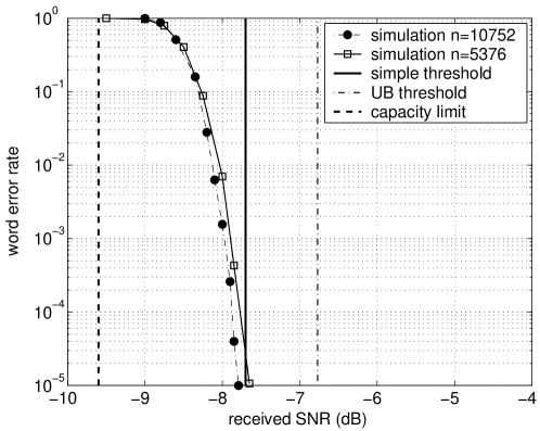
Figure 3: UB and simple code thresholds for an AWGN channel (turbo code of rate $R=1/7$ and length $N=5376$, $10752$)

The component code transfer functions are

$$G_{1}=(1,\,13/15,\,17/15)\text{ and }G_{2}=G_{3}=(13/15,\,17/15).$$

We compute the AWE based on the technique in [22]. By applying (11) and (15), we calculate the UB threshold $c_{0}^{[\mathcal{TC}]}\approx 0.21$ and the simple threshold $c_{\star}^{[\mathcal{TC}]}\approx 0.17$. As shown in Fig. 3, we compare UB and simple thresholds with simulation results for codeword length $N=5376$ and $N=10752$ under iterative decoding when the turbo codes are transmitted over a BI-AWGN channel. Fig. 3 illustrates that the cliff of WER curves becomes sharp as the codeword length $N$ increases. We observe that the simple threshold predicts well the cliff of the simulated word error probability, and that the gap between $c_{0}^{[\mathcal{TC}]}$ and $c_{\star}^{[\mathcal{TC}]}$ is almost $1$ dB. We also consider the capacity limit of the BI-AWGN channel. To this end, we set $C(\lambda)$ in (6) equal to the code rate $R$, and determine the capacity threshold SNR. Fig. 3 illustrates that the capacity threshold may not predict well the error performance of turbo codes.

III-C3 Punctured Code Threshold

For punctured codes, we may assume that punctured bits are sent to a dummy memoryless component channel whose output is independent of the input, i.e., $\gamma_{p}=1$, whereas, non-punctured bits are transmitted over the real channel with the Bhattacharyya parameter $\gamma$. Let the puncturing rate be $1-\tau$, the average Bhattacharyya parameter is $\bar{\gamma}=\gamma\cdot\tau+1\cdot(1-\tau)$. Hence, we can rewrite the reliable communication condition (21) as

$$\gamma<\frac{\exp(-c_{\star})-(1-\tau)}{\tau}.$$ (22)

Analogous to Theorem 1, we have the following result for a (randomly) punctured code ensemble.

Theorem 2

Consider a good codes ensemble $[{\mathcal{C}}]$ with a finite code threshold $c_{\star}$ defined in (15). Assume that the coded symbols are randomly and independently punctured, so that each bit is punctured with a-priori probability (punctured rate) $1-\tau$. If $\tau>1-\exp(-c_{\star})$, there exists a punctured code threshold

$$\chi(\tau)=\ln\frac{\tau}{\exp(-c_{\star})-(1-\tau)}$$ (23)

such that, if

$$-\ln\gamma>\chi(\tau),$$ (24)

the average ML decoding word error probability approaches zero as $N\rightarrow\infty$.

Proof.

The proof follows in a straightforward manner from Theorem 1 and (22). ∎

We note that the left hand side of (24) is the channel Bhattacharyya distance, which is equal to the received SNR for a BI-AWGN channel.

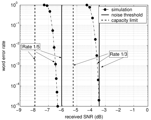
Figure 4: UB and simple code thresholds for an AWGN channel (mother turbo code of $R=1/7$ and $N=26880$)

Thus, the simple code threshold is an SNR threshold for an AWGN channel, i.e., if the received SNR is larger than the punctured code threshold $\chi(\tau)$, the average ML decoding word error probability decays to zero as the codeword length $N$ tends to infinity. We show the SNR threshold behavior of punctured turbo codes in the following example.

Example 2 (threshold for punctured turbo codes)

We consider an example punctured turbo code transmitted over a BI-AWGN channel. The mother turbo code of rate $R=1/7$ and length $N=26880$ is described in Example 1. We study the word error probability performance of its punctured versions of rate $R_{p}=1/5$ (by setting $\tau=5/7$) and $R_{p}=1/3$ (by setting $\tau=3/7$). Based on the simple threshold $c_{\star}^{[\mathcal{TC}]}\approx 0.17$, we calculate the punctured code thresholds $\chi(5/7)\approx 0.25$ and $\chi(3/7)\approx 0.45$. As shown in Fig. 4, we compare the simulation results with punctured thresholds and capacity SNR limits corresponding to $C=1/5$ and $C=1/3$. Fig. 4 illustrates that our punctured code thresholds are in a very good agreement with the numerical value observed in the simulation.

Remark 2

Self-Decodable Condition: Theorem 2 illustrates that if

$$\tau>1-\exp(-c_{\star}),$$ (25)

then the punctured code threshold $\chi(\tau)$ exists for a good mother code ensemble $[{\mathcal{C}}]$. It implies that (25) is a necessary condition which guarantees that a randomly chosen code (sequence) from the punctured code ensemble is self-decodable with probability one. Hence, we refer to (25) as a self-decodable condition.

IV IR Cooperative Coding Scheme

In this section, we introduce an IR coding collaboration scheme. We assume that the sender and helpers acquire a common time reference and operate in a single radio frequency band $W$. The medium access control (MAC) scheme is based on a time-division scheme. The transmission interval $T$ is partitioned into $M$ non-overlapping slots of duration $\tau_{0}T,\dots,\tau_{M-1}T$, where $\tau_{j}$, for $j=0,\dots,M-1$, is referred to as the assignment rate for slot $j$, $\sum_{j=0}^{M-1}\tau_{j}=1,$ and the time allocation $\{\tau_{0},\dots,\tau_{M-1}\}$ is predetermined for all nodes.

Each node in the wireless network has an encoder (associated a codebook $\{{\mathcal{C}}\}$ of length $N$ and rate $R$), a decoder, and a mapping device. The sender (Node $0$) encodes the information and obtains a mother codeword ${\mathcal{C}}$. The mapping device partitions the codeword ${\mathcal{C}}$ into $M$ blocks corresponding to $M$ non-overlapping slots. Block $j$ of length $\tau_{j}N$ is transmitted in slot $j$, $j=0,\dots,M-1$. For analysis simplicity, the partition is based on random assignment [24] which can be described using a probabilistic mapping device which randomly assigns bits of the transmitted codeword to $M$ blocks. More precisely, the random mapper takes a bit of the codeword ${\mathcal{C}}$ and sends it to slot $j$ with a predetermined assignment rate $\tau_{j}$. Bit assignments are independent and, thus, the expected (and asymptotic as $N\rightarrow\infty$) number of bits assigned to block $j$ is $\tau_{j}N$.

After random mapping, each block of bits forms a codeword obtained by puncturing. Let $\mathcal{C}_{j}$ denote the punctured codeword corresponding to slot $j$. For a given good (mother) code ensemble $[{\mathcal{C}}]$ and the (random) assignment rate $\tau_{j}$, Theorem 2 shows that the punctured code ensemble exhibits the SNR threshold behavior for an AWGN channel, i.e., if the received SNR is larger than the punctured code threshold $\chi(\tau_{j})$, the average ML decoding word error probability decays to zero as the codeword length $N$ tends to infinity. As illustrated in (23), the punctured code threshold $\chi(\tau_{j})$ can easily be calculated based on the mother code threshold $c_{\star}$. Hence, this threshold behavior allows for adaptively scheduling the cooperation in two stages described below.

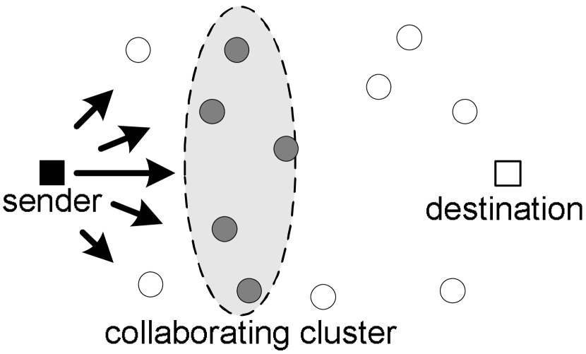
a. slot $0$: sender broadcasts message

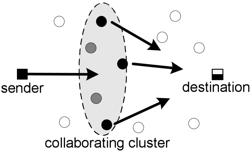
b. slot $1~{}$- slot $M-1$: reliable nodes relay information

Figure 5: Cooperative coding scheme

IV-A Broadcast Stage

As shown in Fig. 5.a, the sender broadcasts its information by transmitting ${\mathcal{C}}_{0}$ during slot $0$. Each helper listens and attempts to decode this message. More precisely, helpers estimate the instantaneous received SNR from the incoming signal and compare the SNR with the punctured code threshold $\chi(\tau_{0})$ corresponding to ${\mathcal{C}}_{0}$ at the beginning of the broadcast stage. Let ${\mathcal{F}}\subseteq{\mathcal{S}}$ denote the reliable set of cluster members whose sender-to-helper instantaneous SNR $\theta_{0,j}>\chi(\tau_{0})$. The element of $\mathcal{F}$ is referred to as the reliable node. The punctured code threshold theorem and quasi-static channel assumption imply that reliable nodes can be guaranteed to decode the message successfully under ML decoding. Next, each reliable node sends an ACK back to the sender over a fast and error-free feedback channel without a need for prior decoding. During this slot, reliable nodes listen and decode the received signal.

IV-B Forwarding Stage

Fig. 5.b illustrates the transmission interval corresponding to slots $1$ through $M-1$ (here, dark solid circles represent reliable nodes). Node $k\in\mathcal{F}$, re-encodes and partitions received information in the same manner as done by the sender and, consequently, relays ${\mathcal{C}}_{k}$ (corresponding to block $k$) to the destination in slot $k$. The sender transmits the left-over blocks in the remaining transmission slots based on received ACKs. The signal received at the destination corresponds to an IR scheme with a fixed number of retransmissions, where a retransmission may experience a different channel quality.

Example 3

Let’s assume $M=5$, Node $0$ is the sender, the collaborative cluster $\mathcal{S}=\{1,2,3,4\}$, and the reliable set $\mathcal{F}=\{1,3\}$. Based on the ACK-based feedback from the cluster, the dynamic schedule is shown in Table I. Since Nodes $1$ and $3$ are reliable nodes, they send ${\mathcal{C}}_{1}$ and ${\mathcal{C}}_{3}$ at Slots $1$ and $3$, respectively. The remaining blocks are transmitted by Node $0$ at Slots $0$, $2$, and $4$.

TABLE I: Dynamic schedule ($M=5$ and $\mathcal{F}=\{1,3\}$)

Slot	$0$	$1$	$2$	$3$	$4$
Transmitted block	${\mathcal{C}}_{0}$	${\mathcal{C}}_{1}$	${\mathcal{C}}_{2}$	${\mathcal{C}}_{3}$	${\mathcal{C}}_{4}$
Transmitter	Node $0$	Node $1$	Node $0$	Node $3$	Node $0$

Remark 3

Decoding Delay: We note that each reliable node needs to decode the message before it relays this information. This results in a decoding delay in the transmission. If one of the reliable nodes is scheduled to send the message in slot $1$, it requires some extra time $\tau_{D}\cdot T$ between slot $0$ and slot $1$ due to a decoding latency. In Appendix -F, we propose both early stopping and a threshold adjusting technique to reduce this time in practice. For simplicity of the error performance analysis, we assume $\tau_{D}=0$ in Sec. V.

Remark 4

Decoding Failure: Since the assignment rate $\tau_{0}$ is predetermined, each helper can pre-calculate the punctured code threshold $\chi(\tau_{0})$ by using (23). On the other hand, Node $j$ may estimate the instantaneous received SNR $\theta_{0,j}$ at the beginning of slot $0$. In our proposed scheme, if $\theta_{0,j}>\chi(\tau_{0})$, Node $j$ is called reliable node and sends an ACK message to the sender. Next, if Node $j$ fails in decoding the message, this node will stay silent during the forwarding stage. We refer to this event as the decoding failure. However, Theorem 2 implies that the probability of such events approaches zero as the codeword length $N\rightarrow\infty$. In this paper, we focus on long codes. Hence, we neglect the decoding failure event in the error performance analysis.

V IR Cooperative Coding Performance Based on Code Outage

The decoding is performed at the destination upon completion of $M$ transmission slots. The proposed cooperative coding scheme implies that the received signal is always the mother codeword ${\mathcal{C}}$ modified by the fading channel. Moreover, all communication links experience independent quasi-static Rayleigh fading channels. Thus, the codeword ${\mathcal{C}}$ is, equivalently, transmitted over $M$ slots and experiences $|\mathcal{F}|+1$ independent channel gains. Consequently, we study the performance of codes transmitted over a block fading channel [20, 15].

V-A Code Outage for a $Q$-Block Fading Channel

Here, we consider the block-fading channel model [20] with $Q$ fading blocks (a group of $Q$ blocks will be referred to as a frame), where the fading coefficient is essentially invariant during a single block and different from one block to another. Let ${\sf SNR}_{j}$ and $\nu_{j}$ be the the average received SNR and the channel power of block $j$, respectively. The Bhattacharyya parameter $\gamma_{j}$ is a function of ${\sf SNR}_{j}$ and $\nu_{j}$, i.e.,

$$\gamma_{j}=\exp(-\nu_{j}\cdot{\sf SNR}_{j})\quad\text{for}\quad j=0,\dots,Q-1.$$

Hence, the average Bhattacharyya parameter over $Q$ blocks

$$\bar{\gamma}(\mbox{\boldmath$\nu$})=\sum_{j=0}^{Q-1}\tau_{j}\gamma_{j}=\sum_{j=0}^{Q-1}\tau_{j}\exp(-\nu_{j}\cdot{\sf SNR}_{j})$$

is a function of the random vector $\mbox{\boldmath$\nu$}\triangleq\{\nu_{0},\dots,\nu_{Q-1}\}$ and, thus, for a given good code, there is a non-negligible probability that the effective Bhattacharyya distance $-\ln\bar{\gamma}(\mbox{\boldmath$\nu$})$ is less than the code threshold $c_{\star}$, termed code outage probability. Thus, the average frame error probability is a function of both the fading distribution and the threshold of the code ensemble $[{\mathcal{C}}]$. More precisely, the average ML decoding word error probability for a good code ensemble $[{\mathcal{C}}]$ transmitted over a $Q$-block fading channel can be bounded as follows:

$$\bar{P}_{W}(\bar{\gamma},N) \triangleq{\sf E}\bigl{[}P_{W}(\bar{\gamma},N)\bigr{]}$$

$$={\rm P}\{{\rm error}(N),\,-\ln\bar{\gamma}(\mbox{\boldmath$\nu$})\leq c_{\star}\}+{\rm P}\{{\rm error}(N),\,-\ln\bar{\gamma}(\mbox{\boldmath$\nu$})>c_{\star}\}$$

$$\leq{\rm P}\{-\ln\bar{\gamma}(\mbox{\boldmath$\nu$})\leq c_{\star}\}+{\rm P}\{{\rm error}(N)\,|-\ln\bar{\gamma}(\mbox{\boldmath$\nu$})>c_{\star}\}$$ (26)

where ${\rm error}(N)$ stands for the event of the decoding error for the code of length $N$. Theorem 1 implies that the second term of (26) approaches zero as the code length $N$ increases. Hence, the following error rate bound holds

$$\bar{P}_{W}(\bar{\gamma},N) \leq{\rm P}\{\bar{\gamma}(\mbox{\boldmath$\nu$})\geq\exp(-c_{\star})\}+o(1)$$ (27)

where $o(1)\stackrel{{\scriptstyle N}}{{\longrightarrow}}0$. We focus on long codes in the following analysis. To simplify notation, we will omit $N$ and $o(1)$.

V-B IR Cooperative Coding Performance

Here we study the FER performance of the IR cooperative coding scheme for a quasi-static frequency-flat Rayleigh-fading channel based on the code outage upper bound (27).

In slot $0$, the sender (Node $0$) broadcasts its information by sending the punctured codeword ${\mathcal{C}}_{0}$. The channel powers $\nu_{0,j}$, $j=1,\dots,M-1$, are i.i.d. exponential random variables invariant during each transmission period. The reliable set ${\mathcal{F}}$ is now randomly distributed over the collection of $2^{M-1}$ subsets of ${\mathcal{S}}$ with probability

$${\rm P}(\mathcal{F}) =\prod_{j\in\mathcal{F}}{\rm P}\{\theta_{0,j}>\chi(\tau_{0})\}\prod_{j\in{\mathcal{F}}^{c}}{\rm P}\{\theta_{0,j}\leq\chi(\tau_{0})\}$$

$$=\prod_{j\in\mathcal{F}}\exp\bigl{[}-\chi(\tau_{0}){\sf SNR}_{0,j}^{-1}\bigr{]}\prod_{j\in{\mathcal{F}}^{c}}\bigl{\{}1-\exp\bigl{[}-\chi(\tau_{0}){\sf SNR}_{0,j}^{-1}\bigr{]}\bigr{\}},$$ (28)

where ${\mathcal{F}}^{c}\triangleq{\mathcal{S}}\setminus{\mathcal{F}}.$

For a given $\mathcal{F}$, the IR cooperation scheme allows the mother codeword to be transmitted to the destination (Node $M$) over $M$ slots with $|\mathcal{F}|+1$ independent quasi-static fading gains. Hence, the slot $i$ Bhattacharyya parameter is

$$\gamma_{i}=\left\{\begin{array}[]{cl}\exp(-\theta_{i,M})&i\in\mathcal{F},\\ \exp(-\theta_{0,M})&i\in{\mathcal{F}}^{c}\cup\{0\}.\end{array}\right.$$ (31)

Consequently, the Bhattacharyya parameter averaged over $M$ slots is now

$$\bar{\gamma}(\mbox{\boldmath$\nu$},\mathcal{F}) =\bigl{(}1-\sum_{i\in\mathcal{F}}\,\tau_{i}\bigr{)}\exp(-\theta_{0,M})+\sum_{i\in\mathcal{F}}\,\tau_{i}\exp(-\theta_{i,M})$$

$$=\bigl{(}1-\sum_{i\in\mathcal{F}}\,\tau_{i}\bigr{)}\exp(-\nu_{0,M}{\sf SNR}_{0,M})+\sum_{i\in\mathcal{F}}\,\tau_{i}\exp(-\nu_{i,M}{\sf SNR}_{i,M}),$$ (32)

where $\mbox{\boldmath$\nu$}=\{\nu_{0,M},\nu_{1,M}\dots,\nu_{M-1,M}\}$ is a random vector $M$-tuple with an independent exponential distribution. The bound (27) implies that the conditional average word error probability given a reliable set $\mathcal{F}$ can be bounded as

$$\bar{P}_{W}\bigl{(}\bar{\gamma}\;|\;{\mathcal{F}}\bigr{)} \leq{\rm P}\bigl{\{}\bar{\gamma}(\mbox{\boldmath$\nu$},\mathcal{F})\geq\exp(-c_{\star})\bigr{\}}=\int_{\mathcal{A}}\,\prod_{i=0}^{M-1}e^{-\nu_{i,M}}\,d\mbox{\boldmath$\nu$}$$

$$\triangleq{\mathcal{G}}(M,\mathcal{F},\mbox{\boldmath${\sf SNR}$})$$ (33)

where $\mathcal{A}\triangleq\bigr{\{}\mbox{\boldmath$\nu$}:\;\bar{\gamma}(\mbox{\boldmath$\nu$},\mathcal{F})\geq\exp(-c_{\star})\bigl{\}}$, $\mbox{\boldmath${\sf SNR}$}=\{{\sf SNR}_{0,M},\dots,{\sf SNR}_{M-1,M}\}$, and ${\mathcal{G}}(M,\mathcal{F},\mbox{\boldmath${\sf SNR}$})$ is referred to as the code outage probability for a given reliable set $\mathcal{F}$. The ML decoding FER for cooperative coding scheme averaged over all possible reliable sets can be bounded as follows

$$\textsf{FER}^{(M)} =\sum_{\text{all possible}~{}\mathcal{F}}{\rm P}(\mathcal{F})\bar{P}_{W}\bigl{(}\bar{\gamma}\;|\;{\mathcal{F}}\bigr{)}\leq\sum_{\text{all possible}~{}\mathcal{F}}{\rm P}(\mathcal{F})\cdot{\mathcal{G}}(M,\mathcal{F},\mbox{\boldmath${\sf SNR}$})$$ (34)

where the superscript $(M)$ represents the number of (potential) transmitting nodes.

Example 4 ($M=1$)

The case $M=1$ is equivalent to the traditional direct transmission between the sender and the destination, and the single-hop FER is

$$\textsf{FER}^{(1)} \leq{\mathcal{G}}(1,\emptyset,{\sf SNR}_{0,1})$$

$$={\rm P}\{\nu_{0,1}{\sf SNR}_{0,1}\leq c_{\star}\}$$

$$=1-\exp(-c_{\star}{\sf SNR}_{0,1}^{-1}).$$ (35)

Example 5 ($M=2$)

Here we consider the IR cooperative coding scheme with a single helper. In this case, the scheme FER is

$$\textsf{FER}^{(2)} \leq{\rm P}(\mathcal{F}=\emptyset)\bar{P}_{W}\bigl{(}\bar{\gamma}\;|\;\emptyset\bigr{)}+{\rm P}(\mathcal{F}=\{1\})\bar{P}_{W}\bigl{(}\bar{\gamma}\;|\;\{1\}\bigr{)}$$

$$=\Bigl{[}1-e^{-\,\chi(\tau){\sf SNR}_{0,1}^{-1}}\Bigl{]}\,{\mathcal{G}}(2,\emptyset,\mbox{\boldmath${\sf SNR}$})+e^{-\,\chi(\tau){\sf SNR}_{0,1}^{-1}}\,{\mathcal{G}}(2,\{1\},\mbox{\boldmath${\sf SNR}$}),$$ (36)

where (assuming $\tau_{0},\tau_{1}\leq\exp(-c_{\star})$)

$${\mathcal{G}}(2,\emptyset,\mbox{\boldmath${\sf SNR}$}) =1-\exp(-c_{\star}{\sf SNR}_{0,2}^{-1})$$ (37)

$${\mathcal{G}}(2,\{1\},\mbox{\boldmath${\sf SNR}$}) =1-\omega-\int_{\omega}^{1}\Bigl{[}\frac{\exp(-c_{\star})-\tau_{0}x^{{\sf SNR}_{0,2}}}{\tau_{1}}\Bigr{]}^{1/{\sf SNR}_{1,2}}\,dx,$$ (38)

$\omega=\exp\bigl{[}-\chi(\tau_{0})\cdot{\sf SNR}_{0,2}^{-1}\bigr{]}$, and the intermediate steps for deriving (38) are given in Appendix -G.

In general, (34) cannot be calculated in a closed form and one needs to resort to numerical integration methods.

VI Asymptotic Analysis

In this section we consider several different cooperation scenarios and derive asymptotic (in SNR) FER bounds, which have a closed form. For simplicity, we assume

$$\tau_{0},\dots,\tau_{M-1}>1-\exp(-c_{\star}).$$ (39)

i.e., each randomly punctured code is self-decodable (with probability one). Next, we refer to $r=\max[d_{0,1},\cdots,d_{0,M-1}]$ as the sender-to-cluster distance, $D=d_{0,M}$ as the sender-to-destination distance, and $d=\max[d_{1,M},\cdots,d_{M-1,M}]$ as the cluster-to-destination distance as shown in Fig 1. Similarly, we define the sender-to-cluster SNR, the sender-to-destination SNR, and the cluster-to-destination SNR as

$$\rho\triangleq E\cdot r^{-L},~{}~{}\eta=E\cdot D^{-L},~{}~{}\text{and}~{}~{}\lambda\triangleq E\cdot d^{-L}.$$ (40)

Computing FER bound (34) requires integration in ${\mathcal{G}}(M,\mathcal{F},\mbox{\boldmath${\sf SNR}$})$, which presents the code outage probability for a given $\mathcal{F}$. The following theorem which is the basis of our asymptotic analysis, among their contributions, helps in avoiding this integration.

Theorem 3

Consider $Q$ independent random variables $\phi_{1},\dots,\phi_{Q}$ with the following properties:

$$0<\phi_{m}\leq 1\quad\text{for}~{}m=1,\dots,Q$$

where the probability distribution of $\phi_{m}$ is a function of $\lambda_{m}$ such that

$$\lim_{\lambda_{m}\rightarrow\infty}\lambda_{m}\,{\rm P}\bigl{[}\phi_{m}>c\bigr{]}=-\ln c$$ (41)

and $0<c<1$. If $\tau_{1},\dots,\tau_{Q}>1-c$ and $\sum_{m=1}^{Q}\tau_{m}=1,$ then

$$\limsup_{\lambda_{1},\dots,\lambda_{Q}\rightarrow\infty}\prod_{m=1}^{Q}\lambda_{m}{\rm P}\left[\sum_{m=1}^{Q}\tau_{m}\phi_{m}>c\right]\leq\frac{1}{Q!}\prod_{m=1}^{Q}\ln\frac{\tau_{m}}{c-(1-\tau_{m})},$$ (42)

where $\lambda_{1},\dots,\lambda_{Q}\rightarrow\infty$ means $\lambda_{1}\rightarrow\infty,\dots,\lambda_{Q}\rightarrow\infty.$

Proof.

The proof is provided in Appendix -H based on the induction method. ∎

VI-A Transmitter Clustering

In the transmitter clustering scenario we assume that $M-1$ helpers are very close to the sender so that $r\rightarrow 0$. For this setting, we call the sender-to-cluster channel fully reliable in the sense of ${\rm P}({\mathcal{F}}=\{1,\dots,M-1\})=1,$ i.e., all helpers are reliable nodes with probability one. Thus, the cooperation scheme FER can be written as

$$\textsf{FER}^{(M)}_{\rm T} =\bar{P}_{W}\bigl{(}\bar{\gamma}\;|\;{\mathcal{F}}=\{1,\dots,M-1\}\bigr{)}$$

$$\leq{\rm P}\{-\ln\bar{\gamma}(\mbox{\boldmath$\nu$},\{1,\dots,M-1\})\leq c_{\star}\}$$

$$={\mathcal{G}}(M,\mathcal{F}=\{1,\dots,M-1\},\mbox{\boldmath${\sf SNR}$}=\{Ed_{i,M}^{-L}\}).$$ (43)

Now, let’s consider the large SNR case. Note that the exponential distribution of $\nu_{i,M}$ implies that

$$\lim_{{\sf SNR}_{i,M}\rightarrow\infty}\,{\sf SNR}_{i,M}\,{\rm P}\Bigl{[}\exp(-\nu_{i,M}{\sf SNR}_{i,M})\geq\exp(-c_{\star})\Bigr{]}$$

$$= \lim_{{\sf SNR}_{i,M}\rightarrow\infty}\,\frac{1-\exp(-c_{\star}{\sf SNR}_{i,M}^{-1})}{{\sf SNR}_{i,M}^{-1}}$$

$$= c_{\star}.$$ (44)

Thus, (23), (33), (39), and Theorem 3 imply

$$\limsup_{\boldsymbol{{\sf SNR}}\rightarrow\infty}\,\prod_{i=0}^{M-1}{\sf SNR}_{i,M}\cdot{\mathcal{G}}(M,\{1,\dots,M-1\},\mbox{\boldmath${\sf SNR}$})\leq\frac{1}{M!}\prod_{i=0}^{M-1}\chi(\tau_{i}).$$ (45)

For large enough $E$, we can rewrite (43) as

$$\textsf{FER}^{(M)}_{\rm T} \leq_{E}\frac{1}{M!}\prod_{i=0}^{M-1}\chi(\tau_{i}){\sf SNR}_{i,M}^{-1}$$ (46)

$$=\frac{1}{E^{M}M!}\prod_{i=0}^{M-1}\chi(\tau_{i})d_{i,M}^{L}$$ (47)

$$=\frac{D^{ML}}{E^{M}M!}\prod_{i=0}^{M-1}\chi(\tau_{i})$$ (48)

where $\leq_{E}$ means that the inequality holds for sufficiently large $E$, and the last step is based on the triangle inequality $D-r\leq d_{i,M}\leq D+r$ and $r\rightarrow 0$.

VI-B Receiver Clustering

In the receiver clustering scenario we assume that $M-1$ cluster members are very close to the destination so that $d\rightarrow 0$. Note that (39) implies that each block (punctured codeword) is self-decodable with probability one. Hence, the code outage probability is zero for any nonempty reliable set $\mathcal{F}$, i.e,

$${\mathcal{G}}(M,\mathcal{F},\mbox{\boldmath${\sf SNR}$})=0~{}~{}\text{for}~{}\mathcal{F}\neq\emptyset.$$ (49)

Therefore, we can bound the cooperation scheme FER as

$$\textsf{FER}^{(M)}_{\rm R} ={\rm P}({\mathcal{F}}=\emptyset)\bar{P}_{W}^{[\mathcal{C}]}\bigl{(}\bar{\gamma}\;|\;{\mathcal{F}}=\emptyset\bigr{)}$$

$$\leq{\rm P}({\mathcal{F}}=\emptyset){\mathcal{G}}(M,\mathcal{F}=\emptyset,\mbox{\boldmath${\sf SNR}$})$$

$$=\prod_{j=1}^{M-1}\bigl{\{}1-\exp\bigl{[}-\chi(\tau_{0}){\sf SNR}_{0,j}^{-1}\bigr{]}\bigr{\}}\bigl{[}1-\exp(-c_{\star}\eta^{-1})\bigr{]}$$

$$=\prod_{j=1}^{M-1}\bigl{\{}1-\exp\bigl{[}-\chi(\tau_{0})E^{-1}d_{0,j}^{L}\bigr{]}\bigr{\}}\bigl{[}1-\exp(-c_{\star}E^{-1}D^{L})\bigr{]}$$ (50)

Again, we focus on the large SNR case. Note that

$$\lim_{{\sf SNR}\rightarrow\infty}{\sf SNR}\cdot\bigl{[}1-\exp(-a{\sf SNR}^{-1})\bigr{]}=a\quad\text{for}~{}a>0.$$

Hence, for large enough $E$, we can rewrite (50) as

$$\textsf{FER}^{(M)}_{\rm R} \leq_{E}\bigl{[}\chi(\tau_{0})\bigr{]}^{M-1}c_{\star}\cdot\prod_{j=1}^{M}{\sf SNR}_{0,j}^{-1}$$ (51)

$$=\frac{\bigl{[}\chi(\tau_{0})\bigr{]}^{M-1}c_{\star}}{E^{M}}\cdot\prod_{j=1}^{M}d_{0,j}^{L}$$

$$=\frac{\bigl{[}\chi(\tau_{0})\bigr{]}^{M-1}c_{\star}}{E^{M}}\cdot D^{ML}$$ (52)

where the last step follows from the geometric property $D-d\leq d_{0,j}\leq D+d$ and $d\rightarrow 0$.

VI-C Cluster Hopping

Figure 6: Cluster hopping

Here, we assume that $d_{0,1}=\dots=d_{0,M-1}=r>0$ and $d_{1,M}=\dots=d_{M-1,M}=d>0$. The distances $d$, $r$, and $D$ satisfy the triangle inequality as shown in Fig. 6. By using (28) in the high SNR regime, we have

$$\lim_{\boldsymbol{{\sf SNR}}\rightarrow\infty}\prod_{j\in{\mathcal{F}}^{c}\setminus\{0\}}{\sf SNR}_{0,j}\,{\rm P}(\mathcal{F}) =\lim_{\rho\rightarrow\infty}\rho^{M-(|\mathcal{F}|+1)}\,{\rm P}(\mathcal{F})$$

$$=\lim_{\rho\rightarrow\infty}\Biggl{\{}\exp\bigl{[}-\chi(\tau_{0})\rho^{-1}\bigr{]}\Biggr{\}}^{|\mathcal{F}|}\Biggl{\{}\frac{1-\exp(-\chi(\tau_{0})\rho^{-1})}{\rho^{-1}}\Biggr{\}}^{M-(|\mathcal{F}|+1)}$$

$$=[\chi(\tau_{0})]^{M-(|\mathcal{F}|+1)}.$$ (53)

Moreover, (23), (33), (39), (44), and Theorem 3 imply

$$\limsup_{\boldsymbol{{\sf SNR}}\rightarrow\infty}\,\prod_{i\in{\mathcal{F}}\cup\{0\}}{\sf SNR}_{i,M}\cdot{\mathcal{G}}(M,\mathcal{F},\mbox{\boldmath${\sf SNR}$}) =\limsup_{\lambda,\,\eta\rightarrow\infty}(\lambda^{|\mathcal{F}|}\,\eta)\cdot{\mathcal{G}}(M,\mathcal{F},\mbox{\boldmath${\sf SNR}$})$$

$$\leq\frac{\chi(1-\sum_{i\in{\mathcal{F}}}\tau_{i})}{(|\mathcal{F}|+1)!}\prod_{i\in{\mathcal{F}}}\chi(\tau_{i}).$$ (54)

Note that

$${\sf SNR}_{0,M}=\eta=ED^{-L},\quad{\sf SNR}_{0,j} =\rho=Er^{-L},\quad{\sf SNR}_{j,M}=\lambda=Ed^{-L},\quad j=1,\dots,M-1.$$

Hence, for large enough $E$, we can rewrite (34) as

$$\textsf{FER}^{(M)} \leq_{E}\sum_{\mathcal{F}}\Biggl{\{}\frac{[\chi(\tau_{0})]^{M-(|\mathcal{F}|+1)}\chi(1-\sum_{i\in{\mathcal{F}}}\tau_{i})}{(|\mathcal{F}|+1)!}\prod_{i\in{\mathcal{F}}}\chi(\tau_{i})\Biggr{\}}(\rho^{|\mathcal{F}|+1-M}\lambda^{-|\mathcal{F}|}\,\eta^{-1})$$ (55)

$$=\sum_{\mathcal{F}}\underbrace{\Biggl{\{}\frac{[\chi(\tau_{0})]^{M-(|\mathcal{F}|+1)}\chi(1-\sum_{i\in{\mathcal{F}}}\tau_{i})}{(|\mathcal{F}|+1)!}\prod_{i\in{\mathcal{F}}}\chi(\tau_{i})\Biggr{\}}}_{\text{coding advantage}}\cdot\underbrace{(r^{M-|\mathcal{F}|-1}d^{|\mathcal{F}|}\,D)^{L}}_{\text{geometric distance profile}}\cdot E^{-M}.$$ (56)

VI-D Diversity Gain

Following [27], the diversity gain is defined as

$$\textsf{div}\triangleq\lim_{{\sf SNR}\rightarrow\infty}\frac{-\log\textsf{FER}}{\log{\sf SNR}}.$$ (57)

Since our collaborating model is a distributed multiple-input single-output (MISO) system, the maximum achievable diversity gain is $M$. Equations (46), (51), and (55) illustrate that all of the three discussed scenarios: transmitter clustering, receiver clustering, and cluster hopping can achieve the full diversity gain, i.e., $\textsf{div}=M$, in high SNR regime.

VI-E Cooperative Coding Gain

For small $c_{\star}$, we can build the following simple relationship between the punctured code threshold and the mother code threshold $c_{\star}$. Equation (23) implies

$$\lim_{c_{\star}\rightarrow 0}\frac{\chi(\tau)}{c_{\star}} =\lim_{c_{\star}\rightarrow 0}(c_{\star})^{-1}\ln\frac{\tau}{\exp(-c_{\star})-(1-\tau)}=\frac{1}{\tau}.$$ (58)

Thus, we can rewrite (56) as

$$\textsf{FER}^{(M)}\leq_{E,c_{\star}}\sum_{\mathcal{F}}\Biggl{\{}\frac{\bigl{(}c_{\star}\bigr{)}^{M}}{\tau_{0}^{M-(|\mathcal{F}|+1)}(1-\sum_{i\in{\mathcal{F}}}\tau_{i})(\prod_{i\in{\mathcal{F}}}\tau_{i})(|\mathcal{F}|+1)!}\Biggr{\}}\cdot(r^{M-|\mathcal{F}|-1}d^{|\mathcal{F}|}\,D)^{L}\cdot E^{-M}.$$ (59)

where $\leq_{E,\,c_{\star}}$ means that the inequality holds for sufficiently large $E$ and small $c_{\star}$.

Example 6 ($M=1$ limiting case)

$$\textsf{FER}^{(1)}\leq_{E}\,\frac{c_{\star}}{\eta}=\frac{c_{\star}}{E}D^{L}.$$ (60)

Example 7 ($M=2$ limiting case)

$$\textsf{FER}^{(2)}\leq_{E,\,c_{\star}}\,\frac{\bigl{(}c_{\star}\bigr{)}^{2}}{\tau_{0}\,\eta\,\rho}+\frac{\bigl{(}c_{\star}\bigr{)}^{2}}{2\tau_{0}\tau_{1}\,\eta\,\lambda}=\left(\frac{c_{\star}}{E}\right)^{2}\left[\frac{(r\,D)^{L}}{\tau_{0}}+\frac{(d\,D)^{L}}{2\tau_{0}\tau_{1}}\right].$$ (61)

Similarly, (48) and (52) can be rewritten as

$$\textsf{FER}^{(M)}_{\rm T} \leq_{E,\,c_{\star}}\frac{1}{M!\prod_{i=0}^{M-1}\tau_{i}}\left(\frac{c_{\star}D^{L}}{E}\right)^{M}$$ (62)

$$\textsf{FER}^{(M)}_{\rm R} \leq_{E,\,c_{\star}}\tau_{0}^{-(M-1)}\left(\frac{c_{\star}D^{L}}{E}\right)^{M}.$$ (63)

In [28], the author defines the cooperative coding gain as

$$\textsf{cop}\triangleq\lim_{{\sf SNR}\rightarrow\infty}\frac{\textsf{FER}^{-1/\textsf{div}}}{{\sf SNR}}.$$ (64)

Let the sender-to-destination SNR be the basis, i.e, $\eta={\sf SNR}$. Bounds (62), (63), and (59) imply that the coding gains of transmitter clustering, receiver clustering, and cluster hopping schemes satisfy

$$\lim_{c_{\star}\rightarrow 0}c_{\star}\cdot\textsf{cop}^{(M)}_{\rm T} \geq\left(M!\prod_{i=0}^{M-1}\tau_{i}\right)^{1/M},$$ (65)

$$\lim_{c_{\star}\rightarrow 0}c_{\star}\cdot\textsf{cop}^{(M)}_{\rm R} \geq\tau_{0}^{(M-1)/M},$$ (66)

$$\lim_{c_{\star}\rightarrow 0}c_{\star}\cdot\textsf{cop}^{(M)} \geq\left\{\sum_{\mathcal{F}}\frac{\bigl{[}(r/D)^{M-|\mathcal{F}|-1}(d/D)^{|\mathcal{F}|}\bigr{]}^{L}}{\tau_{0}^{M-(|\mathcal{F}|+1)}(1-\sum_{i\in{\mathcal{F}}}\tau_{i})(\prod_{i\in{\mathcal{F}}}\tau_{i})(|\mathcal{F}|+1)!}\right\}^{-1/M}.$$ (67)

Inequality (67) illustrates that, in general, the cooperative coding gain is a function of the code parameter $c_{\star}$, the cooperation scheme parameters $\{\tau_{i}\}$, and the geometric distance profile $(r,\,d,\,D)$ of the network.

VII Simulations and Discussions

VII-A IR Cooperative Turbo Coding

In this subsection we study the error performance of the IR cooperation scheme based on the turbo code described in Example 1. FER simulations consider binary antipodal signaling and an independent flat quasi-static Rayleigh fading for each link.

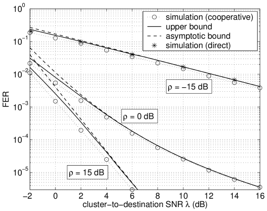
Figure 7: FER vs. $\lambda$ ($M=5$, $\rho=-15,\,0,\,15$, and mother turbo code of rate $R=1/7$ and length $N=5376$)

Each receiver has perfect channel state information and employs coherent detection. All receivers employ a multiple turbo decoder based on the triangle iterative decoding algorithm [29].

Here we consider a $M=5$ collaborative network and assume ${\sf SNR}_{0,1}=\dots={\sf SNR}_{0,4}=\rho$ and $\eta={\sf SNR}_{0,5}=\dots={\sf SNR}_{4,5}=\lambda.$ Thus, the FER performance of cooperative turbo codes is a function of both cluster-to-destination SNR $\rho$ and sender-to-cluster SNR $\lambda$. Fig. 7 depicts the FER for $\rho=-15,\,0,\,15$ dB and as a function of $\lambda$ from $-2$ to $16$ dB.

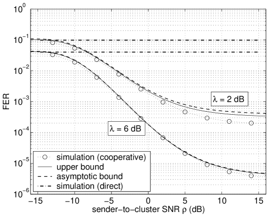
Figure 8: FER performance vs. $\rho$ ($M=5$, $\lambda=2,\,6$, and mother turbo code of rate $R=1/7$ and length $N=5376$)

On the other hand, in Fig. 8, we fix $\lambda=2,6$ dB and study the FER performance vs. sender-to-cluster SNR $\rho$. For these two cases, we compare the simulation result with the analytic upper bound (34) and the asymptotic bound (59). Figs. 7 and 8 also depict the simulation result of the direct transmission as a benchmark. We observe that the upper bound (34) accurately predicts the cooperative coding performance and the asymptotic bound (59) converges to the bound (34) for medium and high SNR. This observation enables us to estimate the FER performance as a function of $\rho$ and $\lambda$ by combining (34) and (59) in Fig. 9, where we use the bound (34) for low SNR and employ the bound (59) to simplify the computation for medium and high SNR.

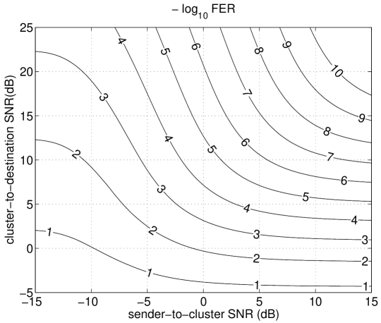
Figure 9: FER performance as a function of $\rho$ and $\lambda$ ($M=5$ and mother turbo code of rate $R=1/7$)

VII-B Collaborative Cluster Size

Here, we study the effect of the collaborative cluster size on the FER performance of the transmitter clustering (the sender-to-cluster distance $r\rightarrow 0$ in this scenario). We assume that nodes have limited battery energy. In this case, achieving high transmission energy efficiency is more important than maximizing the diversity gain. Our approach is to assume that the allowable FER is $\epsilon$, which guarantees the quality of service (QoS), and to determine the $\epsilon$-achievable transmission energy by applying the asymptotic bound studied in Sec. VI. The closed form bound predicts well the error performance for medium and high SNR.

Let $\tau_{0}=\dots=\tau_{M-1}=1/M$, now, (62) implies

$$\textsf{FER}^{(M)}_{\rm T} \leq_{E,\,c_{\star}}\frac{1}{M!}\left(\frac{M\cdot c_{\star}D^{L}}{E^{(M)}}\right)^{M}$$ (68)

where $E^{(M)}$ is the $\epsilon$-achievable transmission energy. To satisfy the QoS requirement, we require

$$\frac{1}{M!}\left(\frac{M\cdot c_{\star}D^{L}}{E^{(M)}}\right)^{M}=\epsilon.$$ (69)

Based on Stirling’s approximation, the $\epsilon$-achievable transmission energy is

$$E^{(M)}\approx\frac{c_{\star}\cdot eD^{L}}{(\epsilon\sqrt{2\pi M})^{1/M}}.$$ (70)

To illustrate how much energy can be saved using the IR cooperative transmission, we consider both direct transmission and transmission over a fully interleaved Rayleigh fading channel cases as benchmarks. For direct transmission (i.e, $M=1$), by using the bound (60) in Example 6, the $\epsilon$-achievable energy is given by

$$E^{(1)}=\frac{c_{\star}\cdot D^{L}}{\epsilon}.$$ (71)

For a fully interleaved Rayleigh fading channel, the Bhattacharyya parameter is a function of the sender-to-destination SNR $\eta$ (see [17] for the detail) as follows

$$\gamma^{({\rm FIRF})}=\frac{1}{1+\eta}$$ (72)

where $({\rm FIRF})$ stands for fully interleaved Rayleigh fading. Theorem 1 implies that the asymptotic word error rate approaches zero (as $N\rightarrow\infty$) if $\gamma^{({\rm FIRF})}<\exp(-c_{\star})$, i.e., the sender-to-destination SNR

$$\eta>\exp(c_{\star})-1.$$

Note that $\eta=E\cdot D^{-L}$. Thus, for this channel, the reliable transmission energy threshold is defined by

$$E^{({\rm FIRF})}\triangleq[\exp(c_{\star})-1]\cdot D^{L}.$$ (73)

Let $U^{(M)}\triangleq E^{(1)}/E^{(M)}$ denote the transmission energy saving. Equations (70) and (71) lead to

$$U^{(M)}\approx\frac{(2\pi M)^{1/2M}}{e\cdot\epsilon^{1-1/M}}$$ (74)

which illustrates the fact that the energy saving $U^{(M)}$ is a function of only $M$ and $\epsilon$ for the transmitter clustering scenario and does not depend on the code threshold $c_{\star}$ and the sender-to-destination distance $D$. In other words, the energy saving of the IR cooperative coding scheme is universal for all good code families and sender-to-destination distances.

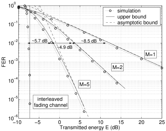
Figure 10: FER vs. transmission energy in the transmitter clustering scenario ($D$=1, ${\rm P}(|\mathcal{F}|=M-1)=1$, and mother turbo code of rate $R=1/7$ and length $N=5376$)

TABLE II: Energy saving vs. $M$

$M$	$2$	$3$	$4$	$5$	${\rm FIRF}$
Estimated $U^{(M)}$ (dB)	$8.4$	$11.1$	$12.4$	$13.2$	$<20$

Next, we set $\epsilon=0.01$ and numerically compute the estimated energy saving in Table II based on the approximation (74). We compare the calculation result with the fully interleaved fading channel savings

$$U^{({\rm FIRF})} =\frac{E^{(1)}}{E^{({\rm FIRF})}}=\frac{c_{\star}}{[\exp(c_{\star})-1]\cdot\epsilon}<1/\epsilon,$$ (75)

where the inequality follows from $\exp(x)>1+x$ for $x>0$. Fig. 10 illustrates the simulated FER performance versus transmission energy $E$ as well as the upper bound (34) and its asymptotic version (59) for $D=1$ and $r\rightarrow 0$. In Fig. 10, we also compare the FER performance of cooperative transmissions vs. transmission over a fully interleaved Rayleigh fading channel. In the latter case, the error performance exhibits a threshold behavior and the reliable transmission energy is described in (73). We observe that the energy saving obtained through simulation (in Fig. 10) and the estimated $U^{(M)}$ (in Table II) illustrate an excellent match. Furthermore, both Table II and Fig. 10 illustrate the fact that, although the cumulative energy saving increases with $M$, the rate of increase drops quickly.

VII-C Normalized Cluster to Destination Distance

Here, we assume $d_{0,1},\dots,d_{0,M-1}=r$, $d_{1,M}=\dots=d_{M-1,M}=d$, $D\thickapprox r+d$ and $\tau_{1}=\dots=\tau_{M-1}$. We move the collaborative cluster from the sender towards the destination, and evaluate the energy saving in terms of the normalized cluster to destination distance $\kappa\triangleq r/D$.

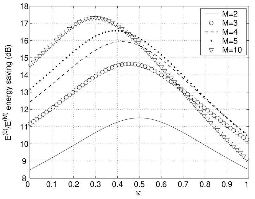
a. $\tau_{0}=1/M$

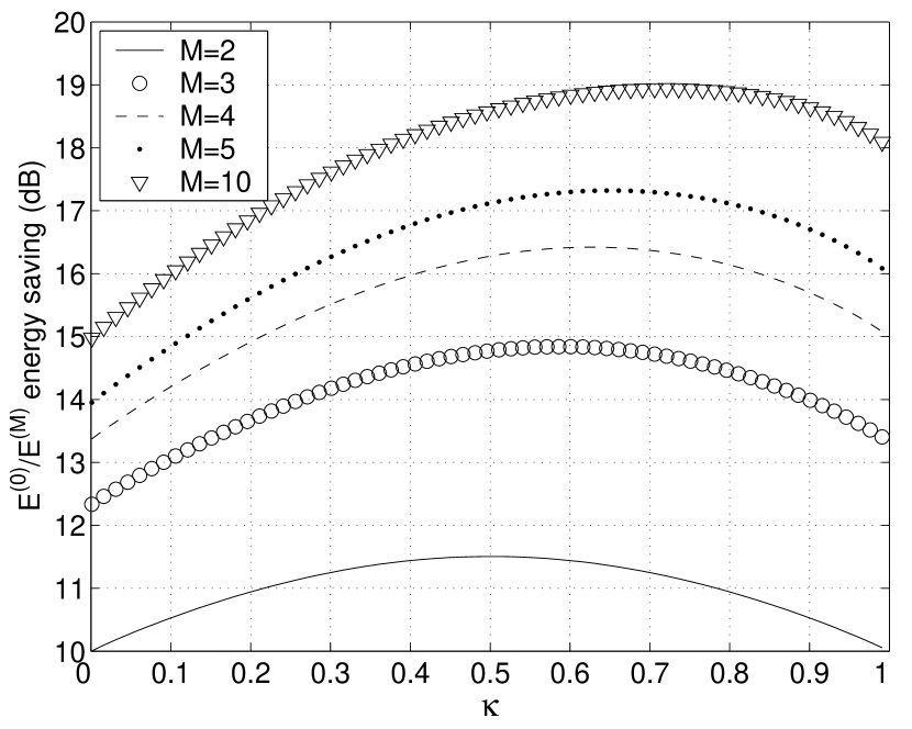
b. optimum $\tau_{0}$

Figure 11: $\epsilon$-achievable transmission energy saving vs. normalized cluster distance $\kappa$ (the required FER $\epsilon=0.01$, path loss exponent $L=3$, $\tau_{j}=(1-\tau_{0})/(M-1)$ for $j\neq 0$)

Here, we use the similar approach as one used in the pervious subsection. We assume that the allowable FER is $\epsilon$ and calculate the the $\epsilon$-achievable energy $E^{(M)}$ based on the asymptotic FER bound (59), i.e.,

$$\sum_{\mathcal{F}}\Biggl{\{}\frac{\bigl{(}c_{\star}\bigr{)}^{M}(r^{M-|\mathcal{F}|-1}d^{|\mathcal{F}|}\,D)^{L}\cdot\bigl{[}E^{(M)}\bigr{]}^{-M}}{\tau_{0}^{M-(|\mathcal{F}|+1)}(1-\sum_{i\in{\mathcal{F}}}\tau_{i})(\prod_{i\in{\mathcal{F}}}\tau_{i})(|\mathcal{F}|+1)!}\Biggr{\}} =\epsilon$$ (76)

Hence, we have

$$E^{(M)}=c_{\star}\cdot D^{L}\Biggl{\{}\frac{1}{\epsilon}\sum_{k=0}^{M-1}\binom{M-1}{k}\frac{\kappa^{L(M-k-1)}(1-\kappa)^{Lk}}{\tau_{0}^{M-(k+1)}\tau_{{\dagger}}^{k}(1-k\tau_{{\dagger}})(k+1)!}\Biggr{\}}^{1/M}$$ (77)

where $\tau_{{\dagger}}=(1-\tau_{0})/(M-1)$. Next, the transmission energy saving $U^{(M)}$ is given by

$$U^{(M)}=\frac{E^{(1)}}{E^{(M)}}=\left\{\epsilon^{M-1}\sum_{k=0}^{M-1}\binom{M-1}{k}\frac{\kappa^{L(M-k-1)}(1-\kappa)^{Lk}}{\tau_{0}^{M-(k+1)}\tau_{{\dagger}}^{k}(1-k\tau_{{\dagger}})(k+1)!}\right\}^{-1/M}.$$ (78)

Equation (78) illustrates that $U^{(M)}$ does not depend on the code threshold $c_{\star}$ and the sender-to-destination distance $D$ for a given $\kappa$. In this sense, we claim that the transmission energy saving of IR cooperative coding schemes is universal.

Based on (78), we depict the transmission energy saving $U^{(M)}$ in Fig. 11 as a function of the normalized cluster distance $\kappa$ for $M=2,$ $3,$ $4,$ $5,$ $10$, where $\epsilon=0.01$, path loss exponent $L=3$, and $0<\kappa<1$. Here, we consider two cases: fixing $\tau_{0}=1/M$ and choosing optimum $\tau_{0}$ for a given $\kappa$. In Fig. 11.a, we observe that $U^{(10)}$ is below $U^{(5)}$ when $\kappa\rightarrow 1$. The reason is that here the assignment rate is fixed to $\tau_{0}=1/M$. We note that $\kappa\rightarrow 1$ implies that the collaborative cluster is close to the destination and far from the sender. In this case, the transmission in slot $0$ (i.e., broadcast stage) is more important (see the receiver clustering case in Sec. VI-B and the asymptotic bound (63)), and larger $\tau_{0}$ helps in increasing the expected number of reliable nodes which relay the message to the destination at the forwarding stage. Hence, we obtain a better energy saving performance for $\tau_{0}=1/4$ than for $\tau_{0}=1/10$ when $\kappa\rightarrow 1$. As a comparison, we depict the energy saving by optimizing $\tau_{0}$ for a given $\kappa$ in Fig. 11.b.

VIII Conclusion

In this paper, we study a cooperative coding scheme for multi-hop wireless networks with incremental redundancy. Threshold analysis of good code ensembles enables the analysis of the IR cooperation coding scheme.

First, we study the threshold behavior of good code ensembles for BISOM Channels. A general relationship among the channel capacity, the Bhattacharyya rate, and cutoff rate is established for BISOM channels. Based on this relationship and the modified Shulman-Feder reliable channel region [15], a simple code threshold is proposed. The reliable communication constraint based on the simple code threshold has the same form as the UB code threshold introduced in [17], but the former result is tighter by almost $1~{}dB$ for an example of a rate $1/7$ turbo code on an AWGN channel.

Next, we consider the fading channel. Based on the code outage concept, a simple threshold bound on FER and its asymptotic version are presented for the IR cooperative coding scheme. The asymptotic bound is a closed form function of the simple code threshold, average channel SNR, geometric distances, and the size of the collaborative network. It enables analysis of the diversity and coding gains for three different scenarios: transmitter clustering, receiver clustering, and cluster hopping.

Finally, we simulate the IR cooperative turbo code performance based on the iterative decoding. Remarkably, our analytical FER bound accurately predicts the simulated cooperative coding performance at any SNR and the asymptotic bound agrees very well with the simulation results at medium and high SNRs. We further discuss the transmission energy gain in terms of collaborative network size and normalized distance for the transmitter clustering and cluster hopping scenarios, respectively. In both cases, we observed that the energy saving does not depend on the sender-to-destination distance and the code threshold. In this sense, we claim that the energy saving of IR cooperative coding scheme is universal for all good code families and all initial non-cooperative hop-distance selections.

-A Modified Shulman-Feder Reliable Channel Region

In this appendix, we state for reference the Modified Shulman-Feder (MSF) reliable channel region for good binary code ensembles transmitted over a set of $Q$ (independent) parallel channels (see [15] for the detail).

Theorem 4 (cf. [15, Theorem 5])

Consider a good binary linear code ensemble $[{\mathcal{C}}]$ of rate $R$ whose transmission takes over $Q$ BISOM parallel channels. Assume that the coded symbols are randomly and independently assigned to these channels, such that each bit is transmitted over Channel $j$ with a-priori probability $\tau_{j}$, for $j=0,\dots,Q-1$, where $\tau_{j}>0$ referred to assignment rate and $\sum_{j=0}^{Q-1}\tau_{j}=1$. Let $C_{j}$ and $\gamma_{j}$ be the channel capacity and the Bhattacharyya parameter of Channel $j$, and $c_{P}$ and $\xi_{P}$ be the restriction UB code threshold and the SF distance defined in (16) and (19), respectively. Then, if the average channel capacity and Bhattacharyya parameter over the $Q$ parallel channels satisfy

$$\sum_{j=0}^{Q-1}\tau_{j}\gamma_{j}<\exp(-c_{P})\quad\text{and}\quad\sum_{j=0}^{Q-1}\tau_{j}C_{j}>R+\xi_{P},$$ (79)

the average ML decoding word error probability decays to zero as the codeword length approaches infinity.

Different from the condition (21) for the simple code threshold, the above MSF reliable channel region (79) requires satisfying two constraints associated with two pairs of channel/code parameters. Hence, this calculation is complex, in particular, when the condition (79) is employed with some practical communication schemes.

-B Some Useful Inequalities

Proposition 1

$\qquad 1+b^{2}\leq 2^{b}\leq 1+b$ for $0\leq b\leq 1$, where the two equalities hold simultaneously when $b=0$ and $b=1$.

Proof.

Let $g(b)=1+b^{2}-2^{b}$. We check the derivatives of $g(b)$ in the region $b\in[0,\,1]$ as follows

$$g^{\prime}(b) =2b-\ln 2\cdot 2^{b},$$

$$g^{\prime\prime}(b) =2-(\ln 2)^{2}\cdot 2^{b}\geq 2\cdot[1-(\ln 2)^{2}]>0,\quad\text{for}~{}0\leq b\leq 1.$$

This means that $g(b)$ is strictly convex. Note that $g(0)=g(1)=0$. Thus, $g(b)<0$ for $b\in(0,\,1)$ and the first inequality of Proposition 1 holds.

Next, let $f(b)=1+b-2^{b}$, we have

$$f^{\prime}(b) =1-\ln 2\cdot 2^{b},$$

$$f^{\prime\prime}(b) =-(\ln 2)^{2}\cdot 2^{b}<0\qquad\text{for}~{}0\leq b\leq 1.$$

This implies that $f(b)$ is strictly concave. Since $f(0)=f(1)=0$, we have $f(b)>0$ for $b\in(0,\,1)$ and the second inequality of Proposition 1 holds. ∎

Proposition 2

$\qquad 2^{-a}+2^{-1/a}\leq 1$ for $a\geq 0,$ where the equality holds when $a=0$, $1$, and $\infty$.

Proof.

Consider $f(a)=2^{-a}+2^{-1/a}$. Due to the symmetry property of the function $f(\cdot)$, i.e., $f(a)=f(1/a)$, we only need to prove $f(a)\leq 1$ for $0\leq a\leq 1.$

Note that $f(a)$ is differentiable and bounded ($0\leq f(a)<2$). Thus, the maximum value of $f(a)$ is either at a boundary point or at a stationary point. Now we check all such kind of points. For boundary points, clearly,

$$f(a)=1\quad\text{when}~{}a=0,1.$$ (80)

By the definition, the stationary point $s$ satisfies

$$f^{\prime}(a)\,\big{|}_{a=s}=-\ln 2\cdot(2^{-s}-\frac{1}{s^{2}}2^{-1/s})=0.$$ (81)

This implies $2^{-1/s}=s^{2}\cdot 2^{-s}$. Thus, for a arbitrary stationary point $s$, we have

$$f(s) =2^{-s}+2^{-1/s}=2^{-s}+s^{2}\cdot 2^{-s}=2^{-s}(1+s^{2})<1~{}~{}~{}\text{for}~{}0<s<1$$ (82)

where the inequality follows from Proposition 1. Hence, (80) and (82) imply the desired result. ∎

-C Proof of Lemma 1

The proof of Lemma 1 is based on Jensen’s inequality [30] and Proposition 1, 2 in Appendix -B.

Proof.

First, we prove $B\leq C$. Note that

$$C-B= -{\sf E}\left\{\log_{2}\left[\frac{p(Y|0)+p(-Y|0)}{p(Y|0)}\cdot 2^{-\sqrt{p(-Y|0)/p(Y|0)}}\Biggl{|}\,0\right]\right\}.$$

Following Jensen’s inequality [30], we have

$$C-B \geq-\log_{2}\left\{\sum_{y}[p(y|0)+p(-y|0)]\cdot 2^{-\sqrt{p(-y|0)/p(y|0)}}\right\}$$

$$=-\log_{2}\Biggl{\{}p(y=0|0)+\sum_{y>0}\bigl{[}p(y|0)+p(-y|0)\bigr{]}\cdot\left[2^{-\sqrt{p(-y|0)/p(y|0)}}+2^{-\sqrt{p(y|0)/p(-y|0)}}\right]\Biggr{\}}.$$ (83)

By using Proposition 2, we have

$$2^{-\sqrt{p(-y|0)/p(y|0)}}+2^{-\sqrt{p(y|0)/p(-y|0)}}\leq 1$$

Hence, (83) can be bounded as

$$C-B \geq-\log_{2}\Bigl{\{}p(y=0|0)+\sum_{y>0}[p(y|0)+p(-y|0)]\Bigr{\}}$$

$$=-\log_{2}1$$

$$=0.$$ (84)

Now, we prove $B\geq R_{0}$. Following Proposition 1, we have

$$\quad\gamma \leq\log_{2}(\gamma+1)\qquad~{}\text{for}~{}0\leq\gamma\leq 1,$$

By the definition of the cutoff rate in (4), we can bound the Bhattacharyya rate as

$$B=1-\gamma\geq 1-\log_{2}(\gamma+1)=R_{0}.$$

By combing (84), we have the desired result. ∎

-D Proof of Lemma 2

The proof of Lemma 2 is by contradiction.

Proof.

We assume that (13) does not hold. Then, there exists a positive $\epsilon_{0}$ such that

$$R>1-\exp(-c_{0})+\epsilon_{0}.$$ (85)

Let’s consider a binary erasure channel (BEC) with erasure probability $p=\exp(-c_{0})-\epsilon_{0}$. Then, the channel capacity and the Bhattacharyya parameter are

$$C(p) \triangleq 1-p=1-\exp(-c_{0})+\epsilon_{0}\quad\text{and}\quad\gamma(p)\triangleq p=\exp(-c_{0})-\epsilon_{0}.$$

Since $\epsilon_{0}>0$, the UB reliable communication condition (14) is satisfied, i.e., $\gamma(p)<\exp(-c_{0})$. Hence, the decoding error probability approaches $0$ as $N\rightarrow 0$. Now, the converse to Shannon’s channel coding theorem [30] implies

$$R\leq C(p)=1-\exp(-c_{0})+\epsilon_{0},$$

which contradicts (85). ∎

-E Proof of Theorem 1

For the proof of Theorem 1 we proceed in the following two steps. We first show the existence of $c_{\star}$ by using Lemma 2. Next, we prove the main result based on the MSF reliable channel region theorem (see Appendix -A) and Lemma 1.

Proof.

Let

$$\Omega\triangleq\{P:~{}1-\exp(-c_{P})\geq R+\xi_{P}~{}\text{and}~{}0\leq P<0.5\}.$$

To prove the existence of $c_{\star}$, we need to show that the set $\Omega$ is not empty. Let’s consider a particular weight partition that $P=0$. In this case, Equations (16) and (19) imply $c_{P}=c_{0}$ and $\xi_{P}=0$. Moreover, Lemma 2 leads to

$$1-\exp(-c_{P})\geq R+\xi_{P}\quad\text{for}\quad P=0.$$

Hence, the set $\Omega\neq\emptyset$ and $c_{\star}$ is well defined.

Next, we prove that, for $\forall~{}P\in\Omega$, $P_{W}(\bar{\gamma},N)\stackrel{{\scriptstyle N}}{{\longrightarrow}}0$ if

$$\bar{\gamma}<\exp(-c_{P})\quad.$$ (86)

The condition (86) implies

$$1-\bar{\gamma}\geq 1-\exp(-c_{P})\geq R+\xi_{P}^{[{\mathcal{C}}]}\quad\text{for}~{}P\in\Omega$$

where the second inquilinity follows from the definition of $\Omega$. On the other hand, Lemma 1 implies that the average channel capacity

$$\bar{C}\triangleq\sum_{j=0}^{Q-1}\tau_{j}C_{j}\geq\sum_{j=1}^{Q-1}(1-\tau_{j}\gamma_{j})=1-\bar{\gamma}.$$

Therefore,

$$\bar{C}>R+\xi_{P}.$$

By combining (86) and Theorem 4, we have the desired result $P_{W}(\bar{\gamma},N)\stackrel{{\scriptstyle N}}{{\longrightarrow}}0$. ∎

-F Discussion on Reducing Decoding Delay

Here, we propose “early stopping” and “threshold adjusting”, which in practice neutralize the effect of decoding delay.

Without of loss generality, we assume that Node $1$ is a reliable node and scheduled to send the message in slot $1$. The key of early stopping is that Node $1$ does not need to listen to the message during the whole slot $[0,\,\tau_{0}T]$, instead, Node $1$ can stop listening early and begin to decode after it receives enough information. Let $\theta_{0,1}$ be the sender-to-helper instantaneous SNR of Node $1$. By the reliable node definition (see Sec. IV-A), we have $\theta_{0,1}>\chi(\tau_{0})$. Hence there exists a effective listening period $\tau^{\prime}$ satisfying

$$\theta_{0,1}>\chi(\tau^{\prime})>\chi(\tau_{0}).$$ (87)

Equations (87) and (23) imply that $\tau^{\prime}$ satisfies

$$\frac{1-\exp(-c_{\star})}{1-\exp(-\theta_{0,1})}<\tau^{\prime}<\tau_{0}.$$

Node $1$ begins to decode after receiving $\tau^{\prime}N$ bits. Theorem 2 implies that the “early stopping” rule can guarantee ML decoding successful at Node $1$. Now, the required extra time is $\tau_{D}+\tau^{\prime}-\tau_{0}$. Clearly, the proposed strategy helps in reducing decoding delay latency.

When $\tau_{D}\ll\tau_{0}$, an alternative method is threshold adjusting. Here, we reset the punctured code threshold to be $\chi(\tau_{0}-\tau_{D})$. We say that Node $1$ is a reliable node (scheduled to send the message in slot $1$) when the sender-to-helper instantaneous SNR

$$\theta_{0,1}>\chi(\tau_{0}-\tau_{D}).$$ (88)

Node $1$ listens to the message during the slot $[0,\,(\tau_{0}-\tau_{D})T]$ and begins to decode after receiving $(\tau_{0}-\tau_{D})N$ bits. Now, there is still $\tau_{D}T$ in slot $0$ for decoding process.

-G Proof of Equation (38)

Here, we provide the intermediate steps for deriving (38).

Proof.

Let

$$x=\exp(-\nu_{0,2})~{}\text{and}~{}y=\exp(-\nu_{1,2}).$$

Recall that fading power gains $\nu_{1,2}$ and $\nu_{0,2}$ are independent exponentially distributed with mean $1$. Hence random variables $x$ and $y$ are independent uniformly distributed over $(0,1]$. By the definition (33), we have

$${\mathcal{G}}(2,\{1\},\mbox{\boldmath${\sf SNR}$}) ={\rm P}\bigl{\{}\tau_{0}\gamma_{0}+\tau_{1}\gamma_{1}\geq\exp(-c_{\star})\bigr{\}}$$

$$=1-{\rm P}\bigl{\{}\tau_{0}\gamma_{0}+\tau_{1}\gamma_{1}<\exp(-c_{\star})\bigr{\}}$$

$$=1-{\rm P}\bigl{\{}\tau_{0}\gamma_{0}+\tau_{1}<\exp(-c_{\star})\bigr{\}}-{\rm P}\bigl{\{}\tau_{0}\gamma_{0}+\tau_{1}\geq\exp(-c_{\star}),\,\tau_{0}\gamma_{0}+\tau_{1}\gamma_{1}<\exp(-c_{\star})\bigr{\}}$$

$$=1-{\rm P}\bigl{\{}\gamma_{0}<\exp[-\chi(\tau_{0})]\bigr{\}}-{\rm P}\Bigl{\{}\gamma_{0}\geq\exp[-\chi(\tau_{0})],\,\gamma_{1}<\frac{\exp(-c_{\star})-\tau_{0}\gamma_{0}}{\tau_{1}}\Bigr{\}}$$ (89)

where the third equality is due to $0\leq\gamma_{1}\leq 1$, and the last equality is based on the definition of punctured code threshold (23). Note that

$$\gamma_{0}=\exp(-\nu_{0,2}{\sf SNR}_{0,2})=x^{{\sf SNR}_{0,2}}$$

$$\gamma_{1}=\exp(-\nu_{1,2}{\sf SNR}_{1,2})=y^{{\sf SNR}_{1,2}}.$$

Hence, the second term of (89) is given by

$${\rm P}\bigl{\{}\gamma_{0}<\exp[-\chi(\tau_{0})]\bigr{\}} ={\rm P}\bigl{\{}x<\omega\bigr{\}}=\omega$$ (90)

where $\omega=\exp\bigl{[}-\chi(\tau_{0})\cdot{\sf SNR}_{0,2}^{-1}\bigr{]}.$ Next, the third term of (89) can be rewritten as

$${\rm P}\Bigl{\{}\gamma_{0}\geq\exp[-\chi(\tau_{0})],\,\gamma_{1}<\frac{\exp(-c_{\star})-\tau_{0}\gamma_{0}}{\tau_{1}}\Bigr{\}} ={\rm P}\Biggl{\{}x\geq\omega,\,y<\Biggl{[}\frac{\exp(-c_{\star})-\tau_{0}x^{{\sf SNR}_{0,2}}}{\tau_{1}}\Biggr{]}^{1/{\sf SNR}_{1,2}}\Biggr{\}}$$

$$=\int_{\omega}^{1}\Biggl{[}\frac{\exp(-c_{\star})-\tau_{0}x^{{\sf SNR}_{0,2}}}{\tau_{1}}\Biggr{]}^{1/{\sf SNR}_{1,2}}\,dx$$ (91)

Combining (89), (90), and (91) together, we have the desired result (38). ∎

-H Proof of Theorem 3

The intuition of the proof of Theorem 3 is described as follows. Since $Q$ is a positive integer, we derive the result based on an induction method. First, we consider the $Q=2$ case and derive Lemma 3 based on a more general setting. Next, we prove the main result of Theorem 3. We show that if the hypothesis (42) holds for the integer $Q=j-1$, it is true for the next greater value $Q=j$.

Lemma 3

Consider two independent random variables $\phi_{1}$ and $\phi_{2}$, where $0\leq\phi_{m}\leq 1$ and the probability distribution of $\phi_{m}$ is a function of $\lambda_{m}$, for $m=1,2$. Assume that

$$\lim_{\lambda_{1}\rightarrow\infty}\lambda_{1}\,{\rm P}[\phi_{1}>c]=f(c),~{}~{}~{}\limsup_{\lambda_{2}\rightarrow\infty}\;\lambda_{2}\,{\rm P}[\phi_{2}>c]\leq h(c),$$ (92)

where $f(c)$ and $h(c)$ are monotone decreasing and integrable, and $f^{\prime}(c)$ is integrable. If

$$0<\tau,\,1-\tau<c,$$

then

$$\limsup_{\lambda_{1},\lambda_{2}\rightarrow\infty}\; \lambda_{1}\lambda_{2}\,{\rm P}[\tau\phi_{1}+(1-\tau)\phi_{2}>c]\leq-\int_{q}^{1}h\Bigl{(}\frac{c-\tau z}{1-\tau}\Bigr{)}f^{\prime}(z)dz$$ (93)

where $q=[c-(1-\tau)]/\tau.$

Lemma 3.

The proof follows the approach in [3]. First, let ${\mathcal{Z}}=\{z_{0},\dots,z_{L}\}$ for some finite $L$ be any partition of the interval $[q,\,1]$ with $z_{0}=q$ and $z_{L}=1$. Next we obtain an outer bound on the event $\{\tau\phi_{1}+(1-\tau)\phi_{2}>c\}$ as

$$\{\tau\phi_{1}+(1-\tau)\phi_{2}>c\} \subseteq\bigcup^{L}_{i=1}\Biggl{\{}\{z_{i-1}\leq\phi_{1}<z_{i}\}\cap\Bigl{\{}\phi_{2}>\frac{c-\tau z_{i}}{1-\tau}\Bigr{\}}\Biggr{\}}$$ (94)

Since $\phi_{1}$ and $\phi_{2}$ are independent, we have

$${\rm P}\Biggl{[}z_{i-1}\leq\phi_{1}<z_{i},~{}\phi_{2}>\frac{c-\tau z_{i}}{1-\tau}\Biggr{]}= \,\Bigl{\{}{\rm P}[\phi_{1}>z_{i-1}]-{\rm P}[\phi_{1}>z_{i}]\Bigr{\}}\,{\rm P}\left[\phi_{2}>\frac{c-\tau z_{i}}{1-\tau}\right]$$ (95)

Hence,

$$\limsup_{\lambda_{1},\lambda_{2}\rightarrow\infty}\lambda_{1}\lambda_{2}\,{\rm P}[\tau\phi_{1}+(1-\tau)\phi_{2}>c] \leq\sum^{L}_{i=1}\limsup_{\lambda_{1},\lambda_{2}\rightarrow\infty}~{}\lambda_{1}\lambda_{2}\,{\rm P}\Biggl{[}z_{i-1}\leq\phi_{1}<z_{i},~{}\phi_{2}>\frac{c-\tau z_{i}}{1-\tau}\Biggr{]}$$

$$\leq\sum^{L}_{i=1}\limsup_{\lambda_{1},\lambda_{2}\rightarrow\infty}\lambda_{1}\Bigl{\{}{\rm P}[\phi_{1}>z_{i-1}]-{\rm P}[\phi_{1}>z_{i}]\Bigr{\}}\cdot\lambda_{2}{\rm P}\Biggl{[}\phi_{2}>\frac{c-\tau z_{i}}{1-\tau}\Biggr{]}$$

$$=\sum^{L}_{i=1}\bigl{[}f(z_{i-1})-f(z_{i})\bigr{]}h\Bigl{(}\frac{c-\tau z_{i}}{1-\tau}\Bigr{)}.$$ (96)

Note that (96) holds for all partitions ${\mathcal{Z}}$ of the interval $[q,\,1]$; and $f(c),$ $f^{\prime}(c),$ and $h(c)$ are all integrable, the supremum of the right-hand side of (96) becomes the integral in (93). ∎

Now, we prove Theorem 3 following the induction method.

Theorem 3.

We first check the $Q=1$ case. Note that $\tau_{1}=1$ in this case, thus, (41) implies the hypothesis (42) holds for $Q=1$.

Next we assume that the hypothesis (42) holds for $Q=j-1$ and consider $Q=j$. Let

$$\tau_{m}^{\prime} =\frac{\tau_{m}}{1-\tau_{j}}\quad\text{for}~{}m=1,\dots,j-1,$$

and

$$f(c) =-\ln c$$

$$h(c) =\frac{1}{(j-1)!}\prod_{m=1}^{j-1}\ln\frac{\tau_{m}^{\prime}}{c-(1-\tau_{m}^{\prime})}.$$

Since $\tau_{m}^{\prime}<1-c$, $\sum_{m=1}^{j-1}\tau_{m}^{\prime}=1$, the induction hypothesis for $Q=j-1$ implies

$$\limsup_{\lambda_{1},\dots,\lambda_{j-1}\rightarrow\infty}\prod_{m=1}^{j-1}\lambda_{m}\cdot{\rm P}\left[\sum_{m=1}^{j-1}\tau_{m}^{\prime}\phi_{m}>c\right]\leq h(c).$$ (97)

Note that $f(c)$ and $h(c)$ are monotone decreasing and integrable, and $f^{\prime}(c)$ is integrable. Then, by Lemma 3,

$$\limsup_{\lambda_{1},\dots,\lambda_{j}\rightarrow\infty}\;\prod_{m=1}^{j}\lambda_{m}\,{\rm P}\left[\sum_{m=1}^{j}\tau_{m}\phi_{m}>c\right]= \ \limsup_{\lambda_{1},\dots,\lambda_{j}\rightarrow\infty}\;\prod_{m=1}^{j}\lambda_{m}\,{\rm P}\left[\tau_{j}\phi_{j}+(1-\tau_{j})\sum_{m=1}^{j-1}\tau_{m}^{\prime}\phi_{m}>c\right]$$

$$\leq \ -\int_{q}^{1}h\Bigl{(}\frac{c-\tau z}{1-\tau}\Bigr{)}f^{\prime}(z)dz$$

$$= \ \frac{1}{(j-1)!}\int_{q}^{1}\frac{1}{z}\,\prod_{m=1}^{j-1}\ln\frac{\tau_{m}}{c-z\tau_{j}-(1-\tau_{j}-\tau_{m})}dz$$ (98)

where

$$q=\frac{c-(1-\tau_{j})}{\tau_{j}}.$$

Since $-\ln z$ is a convex function , Jensen’s inequality implies that

$$\ln\frac{\tau_{m}}{c-z\tau_{j}-(1-\tau_{j}-\tau_{m})} =-\ln\Bigr{[}\frac{z\tau_{j}-c+(1-\tau_{j})}{1-c}\cdot\frac{\tau_{m}-(1-c)}{\tau_{m}}+\frac{\tau_{j}-z\tau_{j}}{1-c}\cdot 1\Bigl{]}$$

$$\leq-\frac{z\tau_{j}-c+(1-\tau_{j})}{1-c}\ln\frac{\tau_{m}-(1-c)}{\tau_{m}}-\frac{\tau_{j}-z\tau_{j}}{1-c}\ln 1$$

$$=\frac{z-q}{1-q}\ln\frac{\tau_{m}}{c-(1-\tau_{m})}\qquad\text{for}~{}~{}q\leq z\leq 1,~{}1\leq m\leq j-1.$$ (99)

Hence,

$$\int_{q}^{1}\frac{1}{z}\,\prod_{m=1}^{j-1}\ln\frac{\tau_{m}}{c-z\tau_{j}-(1-\tau_{j}-\tau_{m})}dz\leq\left[\prod_{m=1}^{j-1}\ln\frac{\tau_{m}}{c-(1-\tau_{m})}\right]\int_{q}^{1}\frac{1}{z}\ \Biggl{[}\frac{z-q}{1-q}\Biggr{]}^{j-1}dz.$$ (100)

Note that $1/z$ and $[(z-q)/(1-q)]^{j-1}$ are, respectively, monotonically decreasing and increasing in $z$. Chebyshev integral inequality [31] implies

$$\int_{q}^{1}\frac{1}{z}\ \Biggl{[}\frac{z-q}{1-q}\Biggr{]}^{j-1}dz \leq\frac{1}{1-q}\int_{q}^{1}\Biggl{[}\frac{z-q}{1-q}\Biggr{]}^{j-1}dz\cdot\int_{q}^{1}\frac{1}{z}dz$$

$$=-\frac{\ln q}{j}.$$ (101)

Finally, by combining (98), (100), and (101), we have the desired result

$$\limsup_{\lambda_{1},\dots,\lambda_{j}\rightarrow\infty}\;\prod_{m=1}^{j}\lambda_{m}\,{\rm P}\left[\sum_{m=1}^{j}\tau_{m}\phi_{m}>c\right] \leq\ \frac{1}{j!}\left[\prod_{m=1}^{j}\ln\frac{\tau_{m}}{c-(1-\tau_{m})}\right].$$ (102)

Since both the baseline case ($Q=1$) and the inductive step ($Q=j$) satisfy (42), we conclude that the hypothesis (42) holds for all $Q$. ∎

References

- [1] A. Sendonaris, E. Erkip, and B. Aazhang, “Increasing uplink capacity via user cooperation diversity,” in Proc. IEEE Int. Symp. Inform. Theory 1998, Cambridge, MA, Aug. 1998, p. 156.
- [2] J. N. Laneman, D. N. C. Tse, and G. W. Wornell, “Cooperative diversity in wireless networks: efficient protocols and outage behavior,” IEEE Trans. Inf. Theory, vol. 50, pp. 3062–3080, Dec. 2004.
- [3] J. N. Laneman and G. W. Wornell, “Distributed space-time-coded protocols for exploiting cooperative diversity in wireless networks,” IEEE Trans. Inf. Theory, vol. 49, pp. 2415–2425, Oct. 2003.
- [4] T. E. Hunter, S. Sanayei, and A. Nosratinia, “Outage analysis of coded cooperation,” IEEE Trans. Inf. Theory, vol. 52, pp. 375–391, Feb. 2006.
- [5] A. Stefanov and E. Erkip, “Cooperative coding for wireless networks,” IEEE Trans. Commun., vol. 52, pp. 1470–1476, Sept. 2004.
- [6] T. E. Hunter and A. Nosratinia, “Diversity through coded cooperation,” IEEE Trans. Wireless Commun., vol. 5, pp. 283–289, Feb. 2006.
- [7] B. Zhao and M. C. Valenti, “Distributed turbo coded diversity for the relay channel,” IEE Electronocs Letters, vol. 39, pp. 786–787, May 2003.
- [8] R. Liu, P. Spasojević, and E. Soljanin, “User cooperation with punctured turbo codes,” in Proc. Allerton Conference on Commun. Contr. Computing, Urbana, IL, Oct. 1–3, 2003. [Online]. Available: http://www.winlab.rutgers.edu/liurh
- [9] M. Janani, A. Hedayat, T. E. Hunter, and A. Nosratinia, “Coded cooperation in wireless communications: Space-time transmission and iterative decoding,” IEEE Trans. on Signal Processing, vol. 52, pp. 362–371, Feb. 2004.
- [10] R. Liu, P. Spasojević, and E. Soljanin, “Cooperative diversity with incremental redundancy turbo coding for quasi-static wireless networks,” in Proc. IEEE International Workshop on Signal Processing Advances for Wireless Communications (SPAWC), New York City, June 2005.
- [11] D. J. C. MacKay, “Good error-correcting codes based on very sparse matrices,” IEEE Trans. Inf. Theory, vol. 45, pp. 399–431, Mar. 1999.
- [12] R. Liu, P. Spasojević, and E. Soljanin, “On the weight spectrum of good linear binary codes,” IEEE Trans. Inf. Theory, vol. 51, pp. 4369–4373, Dec. 2005.
- [13] N. Shulman and M. Feder, “Random coding techniques for nonrandom codes,” IEEE Trans. Inf. Theory, vol. 45, pp. 2101–2104, Sept. 1999.
- [14] G. Miller and D. Burshtein, “Bounds on the maximum-likelihood decoding error probability of low-density parity-check codes,” IEEE Trans. Inf. Theory, vol. 47, pp. 2696–2710, Nov. 2001.
- [15] R. Liu, P. Spasojević, and E. Soljanin, “Reliable channel regions for good codes transmitted over parallel channels,” IEEE Trans. Inf. Theory, vol. 52, pp. 1405–1424, Apr. 2006.
- [16] R. Liu and P. Spasojević, “On the bhattacharyya rate for binary-input symmetric-output memoryless channels and its code threshold,” in Proc. IEEE Inf. Theory Workshop, Chengdu, China, Oct. 2006.
- [17] H. Jin and R. J. McEliece, “Coding theorems for turbo code ensembles,” IEEE Trans. Inf. Theory, vol. 48, pp. 1451–1461, June 2002.
- [18] E. Malkamäki and H. Leib, “Evaluating the performance of convolutional codes over block fading channels,” IEEE Trans. Inf. Theory, vol. 45, pp. 1643–1646, July 1999.
- [19] S. Zhao, Z. Wu, A. Acharya, and D. Raychaudhuri, “PARMA: A PHY/MAC aware routing metric for ad-hoc wireless networks with multi-rate radios,” in IEEE International Symposium on a World of Wireless, Mobile and Multimedia Networks (WoWMoM 2005), Taormina, Italy, June 2005, pp. 286–292.
- [20] E. Biglieri, J. Proakis, and S. Shamai (Shitz), “Fading channels: information-theoretic and communications aspects,” IEEE Trans. Inf. Theory, vol. 44, pp. 1895–1911, Oct. 1998.
- [21] R. G. Gallager, Low-Density Parity-Check codes. Cambridge, MA: MIT Press, 1963.
- [22] D. Divsalar, “A simple tight bound on error probability of block codes with application to turbo codes,” Jet Propulsion Lab, CIT, CA, Tech. Rep. TMO 42-139, Nov. 1999.
- [23] I. Sason, E. Telatar, and R. Urbanke, “On the asymptotic input-output weight distributions and thresholds of convolutional and turbo-like encoders,” IEEE Trans. Inf. Theory, vol. 48, pp. 3052–3061, Dec. 2002.
- [24] E. Soljanin, R. Liu, and P. Spasojević, “Hybrid ARQ with random transmission assignments,” in DIMACS Workshop on Network Information Theory, Piscataway, NJ, Mar. 17–19, 2003, pp. 321–334. [Online]. Available: http://cm.bell-labs.com/cm/ms/who/emina
- [25] L. H. Ozarow, S. Shamai, and A. D. Wyner, “Information theoretic considerations for cellular mobile radio,” IEEE Trans. Veh. Technol., vol. 43, pp. 359–378, May 1994.
- [26] Physical Layer Standard for cdma2000 Spread Spectrum Systems (Revision C), 3GPP2 Std. C.S0002-C, 2004.
- [27] L. Zheng and D. N. C. Tse, “Diversity and multiplexing: a fundamental tradeoff in multiple antenna channels,” IEEE Trans. Inf. Theory, vol. 49, pp. 1073–1096, May 2003.
- [28] J. N. Laneman, “Network coding gain of cooperative diversity,” in Proc. IEEE Military Comm. Conf. (MILCOM), Monterey, CA, Nov. 2004.
- [29] D. Divsalar and F. Pollara, “Multiple turbo codes,” in Proc. IEEE Milit. Commun. Conf., San Diego, CA, Nov. 1995, pp. 279–285.
- [30] T. Cover and J. Thomas, Elements of Information Theory. New York: John Wiley, 1991.
- [31] D. S. Mitrinovic, Anayltic Inequalities. New York: Springer-Verlag, 1970.