Revisiting Evolutionary Algorithms with On-the-Fly Population Size Adjustment

In an evolutionary algorithm, the population has a very important role as its size has direct implications regarding solution quality, speed, and reliability. Theoretical studies have been done in the past to investigate the role of population sizing in evolutionary algorithms. In addition to those studies, several self-adjusting population sizing mechanisms have been proposed in the literature. This paper revisits the latter topic and pays special attention to the genetic algorithm with adaptive population size (APGA), for which several researchers have claimed to be very effective at autonomously (re)sizing the population.

As opposed to those previous claims, this paper suggests a complete opposite view. Specifically, it shows that APGA is not capable of adapting the population size at all. This claim is supported on theoretical grounds and confirmed by computer simulations.

1 Introduction

Evolutionary algorithms (EAs) usually have a number of control parameters that have to be specified in advance before starting the algorithm itself. One of those parameters is the population size, which in traditional EAs is generally set to a specified value by the user at the beginning of the search and remains constant through the entire run. Having to specify this initial parameter value is problematic in many ways. If it is too small the EA may not be able to reach high quality solutions. If it is too large the EA spends too much computational resources. Unfortunately, finding an adequate population size is a difficult task. It has been shown, both theoretically and empirically, that the optimal size is something that differs from problem to problem. Moreover, some researchers have observed that at different stages of a single run, different population sizes might be optimal.

Based on these observations, researchers have suggested various schemes that try to learn a good population size during the EA run itself [Lobo & Lima, 2005]. In a recent study [Eiben, Marchiori, & Valko, 2004], several adaptive population size methods were compared head to head on a set of instances of the multimodal problem generator [Spears, 2002]. The winner of that competition was found to be the genetic algorithm with adaptive population size (APGA) [Bäck, Eiben, & van der Vaart, 2000], where the parameter-less genetic algorithm [Harik & Lobo, 1999] had the worst performance out of 5 contestant algorithms, which included a simple GA with a fixed population size of 100.

This paper revisits the comparison between APGA and the parameter-less GA in what is claimed to be a more fair basis than the one used before. More important, the paper shows that APGA is not capable of adapting the population size, a claim that is supported by theoretical and empirical evidence.

The paper is structured as follows. The next section reviews two adaptive population size methods based on age and lifetime. Then, Section 3 analyzes in detail how one of these algorithms, the APGA, resizes the population through time. In Section 4 the analysis is verified with experimental results. The parameter-less GA is described in Section 5. Section 6 makes a critical note regarding a past comparative study of population (re)sizing methods, and Section 7 performs a comparison between APGA and the parameter-less GA for a class of problems that has well-known population size requirements. The paper finalizes with a summary and conclusions.

2 Adaptive schemes based on age and lifetime

This section reviews two techniques for adapting the population size based on the concept of age and lifetime of an individual. The first method was proposed for adapting the population size of a generational GA, while the second method is an extension of the first to allow adaptive population sizing in a steady-state GA, incorporating also elitism.

2.1 GAVaPS

The Genetic Algorithm with Varying Population Size (GAVaPS) was proposed by ?). The algorithm relies on the concept of age and lifetime of an individual to change the population size from generation to generation. When an individual is created, either during the initial generation or through a variation operator, it has age zero. Then, for each generation that the individual stays alive its age is incremented by 1.

At birth, every individual is assigned a lifetime which corresponds to the number of generations that the individual stays alive in the population. When the age exceeds the individual’s lifetime, the individual dies and is eliminated from the population. Different strategies to allocate lifetime to individuals can be used but the key idea is to allow high-quality individuals to remain in the population for longer number of generations than poor-quality individuals. The authors suggested three different strategies: proportional, linear, and bi-linear allocation. All those strategies relied on two parameters, MinLT and MaxLT, which correspond to the minimum and maximum lifetime value allowable for an individual.

At every generation, a fraction $\rho$ (called the reproduction ratio) of the current population is allowed to reproduce. Every individual of the population has an equal probability of being chosen for reproduction. Thus, GAVaPS does not have an explicit selection operator as traditional GAs do. Instead, selection is achieved indirectly through the lifetime that is assigned to individuals. Those with above-average fitness have higher lifetimes than those with below-average fitness. The idea is that the better an individual is, the more time it should be allowed to stay in the population, and therefore increase the chance to propagate its traits to future individuals. Figure 1 details the pseudo-code of GAVaPS.

 procedure GAVaPS
 begin
   t = 0;
   initialize pop(t);
   evaluate pop(t);
   while not termination-condition do
   begin
      t = t+1;
      pop(t) = pop(t-1);
      increase age of pop(t) members by 1;
      cross and mutate pop(t);
      evaluate pop(t);
      remove from pop(t) all individuals
         with age greater than their lifetime;
   end
 end

Figure 1: Pseudocode of the genetic algorithm with varying population size (GAVaPS).

The authors tested GAVaPS on four test functions, compared its performance with that of a simple GA using a fixed population size, and observed that GAVaPS seemed to incorporate a self-tuning process of the population size. GAVaPS requires the user to specify the initial population size, but the authors refer in their work that GAVaPS is robust with respect to that, i.e., the initial population size seemed to have no influence on the performance on the test functions chosen. The same thing did not hold with the reproduction ratio $\rho$. Different values of $\rho$ yielded different performance of the algorithm. For the MinLT and MaxLT parameters, Arabas et al. used 1 and 7 respectively.

2.2 APGA

The Genetic Algorithm with Adaptive Population Size (APGA) proposed by ?) is a slight variation of the GAVaPS algorithm. The difference between the two is that APGA is a steady-state GA, the best individual in the population does not get older, and in addition to the selection pressure obtained indirectly by the lifetime mechanism, APGA also uses an explicit selection operator for choosing individuals to reproduce. Thus, APGA uses a stronger selection pressure than GAVaPS. An algorithmic description of APGA is presented in Figure 2.

 procedure APGA
 begin
   t = 0;
   initialize pop(t);
   evaluate pop(t);
   compute RLT for all members of pop(t);
   while not termination-condition do
   begin
      t = t+1;
      pop(t) = pop(t-1);
      decrement RLT by 1 for all but
          the best member of pop(t);
      select 2 individuals from pop(t);
      cross and mutate the 2 individuals;
      evaluate the 2 individuals;
      insert the 2 offspring into pop(t);
      remove from pop(t) those members with RLT=0;
      compute RLT for the 2 new members of pop(t);
   end
 end

Figure 2: Pseudocode of the genetic algorithm with adaptive population size (APGA). RLT stands for remaining lifetime.

As opposed to the authors of GAVaPS, ? set the values of MinLT and MaxLT to 1 and 11, because according to them, initial runs with different values indicated that MaxLT=11 delivers good performance. APGA also needs the initial population size to be specified (Bäck et al. used 60 individuals in their experiments).

At every iteration of the steady-state GA, all individuals (except the best one) grow older by 1 unit. Thus, it’s quite likely that after MaxLT iterations, most of the individuals from the original population will have died and the only ones that remain in the population are either: (1) the individuals generated during the last MaxLT iterations, or (2) the best individual from the initial population (recall that the best individual does not get older). In other words, after MaxLT iterations the population size will be of order $\mathcal{O}(MaxLT)$. This argument has been hinted before [Lobo & Lima, 2005] and its correctness is confirmed in the next sections.

By not decreasing the remaining lifetime of the best individual, APGA ends up using elitism because the best individual found so far always remains in the population. In ?), the evolution of the population sizes through time is not shown, but in all the reported experiments, the average population size at the end of the runs were in the range between 7.8 and 14.1, which confirms our reasoning that the population size in APGA tends to be of the same order of MaxLT. We will also confirm this reasoning by performing experiments under different settings to observe how the population size in APGA changes over time.

Similarly to GAVaPS, APGA can also use different lifetime strategies. [Bäck, Eiben, & van der Vaart, 2000] used a bi-linear strategy similar to the one proposed for GAVaPS. The bi-linear strategy is a commonly used strategy. For completeness, the formula is shown below.

$$\left\{\begin{array}[]{ll}MinLT+\eta\frac{fit[i]-MinFit}{AvgFit-MinFit}&\mbox{if $AvgFit\geq fit[i]$}\\ \\ \frac{MinLT+MaxLT}{2}+\eta\frac{fit[i]-AvgFit}{MaxFit-AvgFit}&\mbox{if $AvgFit<fit[i]$}\end{array}\right.$$

where $\eta=(MaxLT-MinLT)/2$.

3 How APGA really works?

Let’s analyze in detail the population resizing mechanism of APGA. Let $P(t)$ be the size of the population at generation $t$. Note that in the pseudocode shown in Figure 2, $P(t)$ refers to the size of the population at the end of the while loop. At every generation 2 new individuals are created. Thus, the size of the population at generation $t$ is given by the following recurrence relation:

$$P(t)=P(t-1)+2-D(t)$$ (1)

where $D(t)$ is the number of individuals which die at generation $t$.

Starting from an initial population size $P(0)$, which is a parameter of the algorithm, it is possible to iterate the recurrence relation and obtain the following expression for the population size at generation t:

$$P(t)=P(0)+2~{}t-\sum_{i=1}^{t}D(i)$$ (2)

The summation $\sum_{i=1}^{t}D(i)$ denotes the number of individuals who die in the first $t$ generations. Based on this observation, it is easy to prove that regardless of the initial population size $P(0)$, the population size after $MaxLT$ generations cannot be greater than $2~{}MaxLT+1$.

Theorem 1.

Regardless of $P(0)$,

$$P(MaxLT)\leq 2~{}MaxLT+1$$

Proof.

With an exception for the best individual, $MaxLT$ is an upper bound on the number of generations than any given individual is allowed to live. Thus, after $MaxLT$ generations we can be sure that all but the best member from the initial population will be dead. That is,

$$\sum_{i=1}^{MaxLT}D(i)\geq P(0)-1$$

Using this result together with equation 2 yields,

$$P(MaxLT) = P(0)+2~{}MaxLT-\sum_{i=1}^{MaxLT}D(i)$$

$$\leq 2~{}MaxLT+1$$

which concludes the proof. ∎

Now let us prove that $2~{}MaxLT+1$ remains an upper bound for the population size for the remaining generations.

Theorem 2.

For all $t\geq MaxLT$,

$$P(t)\leq 2~{}MaxLT+1$$

Proof.

One just needs to notice that the exact same reasoning used to prove Theorem 1 can be used to prove the same thing assuming that the starting point is not the initial generation, but instead, some arbitrary generation $k$. That is, regardless of $P(k)$,

$$P(k+MaxLT)\leq 2~{}MaxLT+1$$

Thus, using induction with $k=0$ as a base case, we prove that the upper bound $2~{}MaxLT+1$ holds for all $k>0$. ∎

The proofs that we have seen are relatively straightforward. Nevertheless, in order to make them more easily understandable, Figure 3 depicts schematically an example (with $P(0)=20$ and $MaxLT=3$) of what might be the state of the population after $MaxLT$ generations have elapsed. The example shown corresponds to the upper bound for the size of the population at generation $maxLT$, which is obtained when all individuals are assigned the maximum lifetime value during their creation. The numbers in the figure denote the remaining lifetime (RLT) of the individuals. When an individual is created it is assigned a RLT of 3. Then, at every generation, 2 new individuals are created (and also assigned an RLT of 3) and the remaining ones have their RLT value decremented by 1. An exception occurs for the best individual of the previous generation. In the example, we are assuming the fourth individual (from left to right) to be the best one. Notice that when going from generation to generation, the new best individual can only be the previous best or one of two newly created solutions. The upper bound of $2~{}MaxLT+1$ corresponds to the situation where the best solution remains the same for the last MaxLT generations, as depicted in the figure.

Figure 3: An example with $MaxLT=3$ of the evolution of the population size in APGA. The numbers in the figure denote an upper bound for the remaining lifetime of the individuals.

In summary, after $MaxLT$ generations, the population size in APGA is upper bounded by $2~{}MaxLT+1$, and from that point on until the end of the search, the population size will not raise beyond that bound.

Notice that what we have shown is an upper bound on the maximum population size. To discover that upper bound we had to be conservative and assume that all individuals that are created are able to stay in the population for $MaxLT$ generations. In practice, what is likely to occur in a real APGA simulation is that the actual population size will be somewhat less than that. Due to the effects of selection, it is not clear what is the expected number of generations that an individual stays in the population, but as a very crude approximation, we could say that it should be a value close to $AvgLT=(MinLT+MaxLT)/2$. This thought experiment, suggests that if we replace $MaxLT$ by $AvgLT$ in the upper bound expression, we can get an approximation of the steady state population size of APGA.

Conjecture 1.

For $t\geq MaxLT$, the size of the population is approximately $MinLT+MaxLT+1$.

$$P(t) \approx 2~{}AvgLT+1$$

$$= 2~{}(MinLT+MaxLT)/2)+1$$

$$= MinLT+MaxLT+1$$

At this point, it is time to do some simulations to confirm the theory.

4 Verifying the theory

APGA was tested on 3 problem instances (1, 50, and 100 peaks) of the multimodal problem generator used by ?). This generator creates problem instances with a controllable number of peaks (the degree of multi-modality). For a problem with $\cal P$ peaks, $\cal P$ $L$-bit strings are randomly generated. Each of these strings is a peak (a local optima) in the landscape. Different heights can be assigned to different peaks based on various schemes (equal height, linear, and so on). To evaluate an arbitrary individual $\bar{x}$, first locate the nearest peak in Hamming space, call it $Peak_{n}(\bar{x})$. Then the fitness of $\bar{x}$ is the number of bits the string has in common with that nearest peak, divided by $L$, and scaled by the height of the nearest peak.

$$f(\bar{x})=\frac{L-Hamming(\bar{x},Peak_{n}(\bar{x}))}{L}\cdot Height(Peak_{n}(\bar{x}))$$

Figures 4, 5, 6, monitor the population size as time goes by using an initial population size of 60, and minimum and maximum lifetime values of 1 and 11 (like suggested by their authors [Bäck, Eiben, & van der Vaart, 2000, Eiben, Marchiori, & Valko, 2004], 1 and 1000, and also 100 and 100. The latter setting was tested deliberately to verify the upper bound for the size of the population. Note that when $MinLT=MaxLT$, all individuals are assign that same value as their lifetime, and that should correspond to the situation where the population size stays as close as possible to the upper bound of $2~{}MaxLT+1$, as depicted schematically in figure 3.

For completeness, we also use the exact same settings for the other parameters and operators as those used by [Eiben, Marchiori, & Valko, 2004]: two-point crossover with $P_{c}=0.9$, bit-flip mutation with $P_{m}=1/L=0.01$, and binary tournament selection.

We have also performed similar experiments starting with an initial population size value of 1000 individuals (see figures 7, 8, 9). Again, the theory is confirmed. Further experiments were also done with the Java implementation provided by ?) at http://www.cs.vu.nl/ci. These latter experiments were done to make sure that no detail was missing from an eventual lack of understanding on our part regarding the mechanics of the algorithm. The results were identical to the ones obtained with our own implementation.

These results constitute a strong evidence that APGA is not capable of adapting the population size. Independently of the problem being solved, after $MaxLT$ generations have elapsed ($2~{}MaxLT$ function evaluations), the population size tends to fluctuate around a value close to $MinLT+MaxLT$. In other words, the parameters $MinLT$ and $MaxLT$ end up acting as a camouflage of the population size.

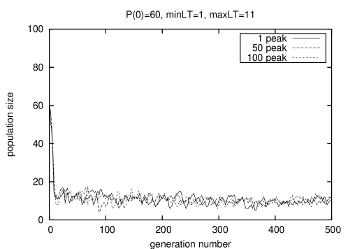
Figure 4: Starting from an initial population size of 60, after $MaxLT=11$ generations the population size is fluctuating around 11 and never raises past $2~{}MaxLT+1=23$.

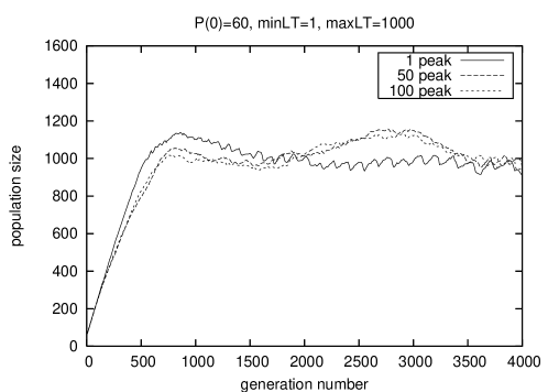
Figure 5: Using $MaxLT=1000$, the population raises initially from 60 to 1000 and then stabilizes around that value.

Figure 6: This example comes very close to the upper bound. Using $MinLT=MaxLT=100$, the population keeps raising by 2 individuals for the first 99 generations. At generation 100, drops to a value of 200 (or 201).

Figure 7: P(0)=1000, MinLT=1, MaxLT=11. Same behavior as in figure 4.

Figure 8: P(0)=1000, MinLT=1, MaxLT=1000. Same behavior as in figure 5.

Figure 9: P(0)=1000, MinLT=100, MaxLT=100. Same behavior as in figure 6.

We now leave APGA for a little while and briefly review another algorithm that does not require the specification of a fixed population size, the parameter-less GA. Later in the paper, both algorithms will tested head-to-head.

5 Parameter-less GA

The parameter-less GA introduced by ?) was developed with the assumption that solution quality grows monotonously with the population size. That is, if after some number of generations $t$, a GA is able to reach a solution quality $q$ with some population size $N_{1}$, then (in a statistical sense) it would also be able to reach that same solution had it started with a population size $N_{2}>N_{1}$. Based on that observation, ? suggested a scheme that simulates an unbounded (potentially infinite) number of populations running in “parallel” with exponentially increasing sizes. Their scheme gives preference to smaller sized populations by allowing them do do more function evaluations than the larger populations. The rationale is that all other things being equal, a smaller sized population should be preferred. After all, if a GA can reach a good solution quality (goodness depends on the stopping criteria, of course) with a population size $N_{1}$, then why bother spending more efforts with a population size $N_{2}>N_{1}$.

Initially the algorithm only has one population whose size is a very small number $N_{0}$ (say 4). As time goes by, new populations are spawned and some can be deleted (more about that later). Thus, at any given point in time, the algorithm maintains a collection of populations. The size of each new population is twice as large as the previous last size. The parameter-less GA does have one parameter! (although ? fixed its value to 4). That parameter (call it $m$) tells how much preference the algorithm gives to smaller populations. Specifically, it tells how many generations are done by a population before the next immediate larger population has a chance to do a single generation.

An example is helpful to illustrate the mechanism. Figure 10 depicts an example with $m=2$. Notice that the number of populations is unbounded. The figure shows the state of the parameter-less GA after 14 iterations. At that point, the algorithm maintains three populations with sizes 4, 8, and 16. Notice how a population of a given size does $m=2$ more generations than the next larger population. In the figure, the numbers inside the rectangles denote the sequence in which the generations are executed by the algorithm. The next step of the algorithm (not shown in the figure) would spawn a new population with size 32.

Figure 10: The parameter-less GA simulates an unbounded number of populations.

This special sequence can be implemented with a $m$-ary counter as suggested by ?), and also with a somewhat simpler implementation as suggested by ?).

In addition to maintaining an unbounded collection of populations, the algorithm uses a heuristic to eliminate populations when certain events occur. In particular, when the average fitness of a population is greater than the average fitness of a smaller sized population, the algorithm eliminates the smaller sized one. The rationale for taking this decision is based on the observation that the larger population appears to be performing better than the smaller one, and it is doing so with less computational resources (recall that the algorithm gives preference to smaller populations). Thus, whenever such an event occurs, ? reasoned that that was a strong evidence that the size of the smaller population was not large enough, and the algorithm should not waste any more time with it. By doing so, the algorithm maintains an invariant that the average fitness of the populations are in decreasing order, with smaller sized populations having higher average fitness than larger populations.

In the absence of mutation, the parameter-less GA also eliminates populations that converge (convergence meaning that the whole population consists of copies of identical individuals) since its not possible to generate new individuals thereafter. Elsewhere it has been shown that the worst case time complexity of the parameter-less GA is only within a logarithmic factor with respect with a GA that starts with an optimal population size [Pelikan & Lobo, 1999].

6 A critical note on experimental research methodology

A comparative study of EAs with on-the-fly population size adjustment has been made in a recent paper [Eiben, Marchiori, & Valko, 2004]. In that study, in addition to APGA and the parameter-less GA, three other algorithms entered the competition: a traditional GA with a fixed population size of 100 (TGA), the GA with random variation of population size (RVPS), and a newly introduced algorithm called PRoFIGA. A description of the algorithms is available elsewhere [Eiben, Marchiori, & Valko, 2004, Lobo & Lima, 2005].

To compare the algorithms, the multimodal random peak problem generator from ?) was used. ? compared the performance of the 5 algorithms on problems with different number of peaks ranging from 1 to 1000. For each problem instance, 100 independent runs were done and the following 3 performance measures were recorded:

• Success Rate (SR), the percentage of runs in which the global optimum was found.

• Mean Best Fitness (MBF), the average of the best fitness in the last population over all runs.

• Average number of Evaluations to a Solution (AES), the number of evaluations it takes on average for the successful runs to find the optimum. If a GA has no success (SR=0) then the AES measure is undefined.

With the exception of population size, all algorithms used the same parameter settings and operators: two-point crossover with $P_{c}=0.9$, bit-flip mutation with $P_{m}=1/L$, binary tournament selection, and delete worst-2 replacement strategy. For all algorithms the GA model was steady-state, not generational.

The experiments were performed on 100-bit string problems and the contestants were allowed to run until either they found the global optimal solution, or a maximum of 10000 function evaluations elapsed. The reader is referred to the original source [Eiben, Marchiori, & Valko, 2004, Valkó, 2003] for more details.

The authors run the experiments and claimed the superiority of APGA, followed closely by PRoFIGA. It is our strong belief that such conclusions are abusive and can be turned upside down very easily. A number of issues should be highlighted.

1. Only allowing the algorithms to run for 10000 function evaluations, is not sufficient to draw any conclusion as to what might happen if the algorithms are allowed to run for longer (or shorter) time spans. The very low success rate obtained for the more difficult problems suggest that the 10000 function evaluations were not sufficient to let the algorithms display their ability in adapting or not the population size.

2. One of the contestants, PRoFIGA, requires the specification of 7 additional parameters that were tuned a-priori for these same problems [Valkó, 2003].

3. The parameter-less GA was not properly implemented because the maximum population size was upper bounded, and the parameter-less GA has no such bound. Quoting ?), “the parameter-less GA is run in parallel with the following 8 population sizes: 2, 4, 8, 16, 32, 64, 128, 256.” In addition to that, the authors should have taken care of only incrementing the 4-base counter after doing $N/2$ generations of the steady state GA ($N$ being the population size) because that is the equivalent of one generation in a generational GA, otherwise large populations are created very quickly violating the principle that more fitness function evaluations are given first to small sized populations.

In addition to the above mentioned flaws, the class of problems generated by the random peak problem generator is probably not the most appropriate for assessing the performance of evolutionary algorithms as shown elsewhere [Lobo & Lima, 2006]. In any case, and for the purpose of demonstrating that the comparative study presented by ? is unfair, let us redo the experiments for 2 instances of the multimodal problem generator, one with 50 and another with 100 peaks. For each instance, 100 independent runs are performed. This time, however, instead of letting the algorithms run until a maximum of 10 thousand function evaluations, we let them run for a maximum of 1 million evaluations.

The APGA uses the exact same settings as those reported by ?: MinLT=1, MaxLT=11, binary tournament selection, 2-point crossover with probability $P_{c}=0.9$, and bit-flip mutation with $P_{m}=1/L=0.01$ The parameter-less GA uses the exact same settings with the exception of the selection rate. It uses a tournament size of 4. The reason why we do so is to make the two algorithms have more or less the same selection pressure (note that APGA has also an extra selection pressure incorporated in its lifetime mechanism). Notice also that in the original parameter-less GA, ? recommended a crossover probability of $P_{c}=0.5$, but we are ignoring those recommendations here in order to run both algorithms under similar conditions. ? also did not give any recommendations regarding mutation rates, but a small mutation rate of $P_{m}=1/L$ cannot possibly do much harm. The performance measures for the 50 and 100 peak problem instances are shown in table 1.

Table 1: APGA versus Parameter-less GA under a maximum of 1 million function evaluations.

Problem	Measure	APGA	Parameter-less GA
	SR	33%	100%
50 peaks	AES	1112	40142
	MBF	0.982	1.000
	SR	17%	96%
100 peaks	AES	1282	74654
	MBF	0.976	0.999

By allowing the algorithms to run for a longer time, the conclusions are completely different from those obtained by ?. On those occasions where APGA reaches the highest peak, it does so very fast. The problem is that APGA is not consistent in reaching the highest peak, not even with 1 million function evaluations. As opposed to that, the parameter-less GA is capable of achieving high success rates, but it can only do it if we give it enough time to do so.

Let us observe now what are were the population sizes needed by both algorithms to reach the highest peak. The population size needed by APGA to reach the highest peak is on average 9.9 (for 50 peaks) and 10.0 (for 100 peaks). That is expected because $MinLT=1$ and $MaxLT=11$. For the parameter-less GA the average population size is 182.5 (for 50 peaks) and 283.4 (for 100 peaks). The parameter-less GA however exhibits a high variance. Sometimes solves the problem as quickly as APGA using a population of size 8, and sometimes needs around 800000 evaluations using a population of 2048.

The reason why this happens is because of the characteristics of the multimodal problem generator. As explained elsewhere [Lobo & Lima, 2006], instances with a large number of peaks can only be solved reliably by an EA if a large population size is used. Otherwise, it can only be solved due to luck, and in those cases, it can be solved very fast, even with a very small population size. The intuition behind this reasoning comes from the observation that when an EA attempts to solve a problem with multiple peaks, it fairly quickly concentrates the population around a single peak. From that point on, the peak can be easily climbed, and obviously it can be climbed faster if a small population size is used. The problem though, is that it is unlikely for the EA to focus its population on the best peak. This reasoning also explains the observation of ? that the AES measure for APGA did not seem much affected by the number of peaks (recall that the AES measure only averages the successful runs).

It should be pointed out that the reason why the parameter-less GA achieved a high success rate in these experiments if not entirely due to its capability of adapting the population size. What is more responsible for the high success rate is the fact that the parameter-less GA maintains a collection of populations, and in effect, each one can be seen as an independent GA run with a different population size. By doing so, the parameter-less GA increases its chances that one of those populations ends up focusing around the basin of attraction of the best peak due to pure luck.

We now look at another type of problem, an instance of an additively decomposable problem, which has well known population sizing requirements [Harik, Cantú-Paz, Goldberg, & Miller, 1999, Goldberg, Deb, & Clark, 1992]. We will be looking at how APGA and the parameter-less GA try to solve the problem.

7 To adapt or not to adapt

Although it can be argued that real world problems are unlikely to be completely decomposable, this class of problems allow researchers to exploit modularity, hierarchy, and bounded difficulty, in a controllable manner. Moreover, this class of problems is the only one for which theoretical population sizing models exist. Thus, they are a natural candidate for testing self-adjusting population sizing mechanisms.

An example of a decomposable problem is a function composed of multiple deceptive sub-functions. Deceptive functions normally have one or more deceptive optima that are far away from the global optimum and which misleads the search in the sense that the attraction area of the deceptive optima is much greater than the one of the optimal solution. A well known deceptive function is the k-trap function [Deb & Goldberg, 1993] defined as follows:

$$f_{trap}(u)=\left\{\begin{array}[]{ll}1&\textrm{if $u$ = $k$}\\ 1-d-u*\frac{1-d}{k-1}&\textrm{otherwise}\end{array}\right.$$ (3)

where $u$ is the number of 1s in the string, $k$ is the size of the trap function, and $d$ is the fitness signal between the global optimum and the deceptive optimum.

If the whole problem is deceptive, there is no way to find the global optimum efficiently by any algorithm because the problem is akin to a needle in a haystack. But if the level of deception is bounded to a few number of bits, the problem becomes solvable by GAs. A commonly used bounded deceptive problem consists of a concatenation of $m$ copies of a $k$-bit trap function. Then, the fitness of a solution is the sum of the contributions of the $m$ trap functions.

$$f(X)=\sum_{i=0}^{m-1}f_{trap}(x_{ki},x_{ki+1},\ldots,x_{ki+k-1}).$$ (4)

On this type of problems, GAs are able to reliably find the global optimum in an efficient way, provided that the population is properly sized [Goldberg, Deb, & Clark, 1992, Harik, Cantú-Paz, Goldberg, & Miller, 1999], and also assuming that the crossover operator is not too disruptive. Since this problem has well known population sizing requirements, it is a natural candidate for testing the ability of EAs incorporating self-adjusting population sizing mechanisms.

We will be testing both APGA and the parameter-less GA on a single instance of the concatenated trap problem, an 80-bit problem consisting of $m=20$ concatenated 4-bit trap functions (we use $d=1/k=0.25$). The goal of the experiments is not to make a strict comparison of the algorithms, nor saying that one is better than the other. Instead, we want to illustrate how the population resizing mechanisms of the algorithms behave on a problem that is known to have minimal population sizing requirements in order to be solved efficiently. For both algorithms we use the same parameter settings as described in the previous section.

We do 100 independent simulations and stop the algorithms either when the global optimum is found, or when a maximum of 1 million function evaluations is reached. The APGA failed to solve a single run to optimality. A reason for that? APGA is not capable of adapting the population size and tries to solve the problem with populations sized around 9-10 individuals, a value of the same order of magnitude as $MaxLT$. The parameter-less GA (we use $m=4$ as in suggested by ?), on the other hand, was able to learn that it had to raise the population well beyond that, and obtained 100% success rate, taking on average 147 thousand function evaluations to reach the global optimum. The population size needed by the parameter-less GA to reach the optimum was on average 840, and the distribution was 256 (2/100 runs), 512 (43/100 runs), 1024 (50/100 runs), and 2048 (5/100 runs).

Figure 11 shows how the ranges of population sizes maintained by the parameter-less GA evolves as time goes by. The figure shows what happens on a single run alone. Other runs have a similar behavior. In the figure there are two lines. The bottom one is for the lowest sized population maintained by the algorithm. The line above it is for the largest sized population maintained by the algorithm at any given point in time. Notice how early in the run, the algorithm is using small sized populations, but fairly quickly it detects that those small sizes are not enough and eliminates them. Each vertical step in the lower line corresponds to an event where a population is deleted (because a larger population has a higher average fitness). Regarding the top line, each vertical step corresponds to an event where a new population is being created for the first time. For example, the population of size 1024 was first created when the algorithm had already spent around 30 thousand evaluations.

Figure 11: Range of population sizes maintained by the parameter-less GA. The dashed line is the minimum population size, and the solid line is the maximum population size maintained by the algorithm at any given point in time.

The lower line represents in some sense the current guess of the parameter-less GA as to what might be a good population size for the problem at hand. In this particular run, the algorithm reached the global optimum with the population size of 1024, and did so after spending a total of 149 thousand function evaluations.

For that same run of the parameter-less GA, figures 12 and 13 show the division of labor (how many function evaluations were spent by each population size) as well as the maximum fitness value reached by each population size through the entire run. In this particular run, the population of size 1024 was able to reach the global optimum. All the other evaluations are in some sense an overhead for the parameter-less GA, a price that it had to pay in order to remove the guessing and tweaking from the user. Notice also how larger populations are able to reach higher fitness values. The exceptions occur with the larger populations (2048 and 4096 in this case) because they are still in their early stages of evolutions and not many evaluations were spent with those population sizes yet.

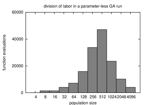
Figure 12: Number of function evaluations spent by each population size during an entire run of the parameter-less GA.

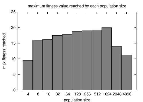
Figure 13: Maximum fitness value reached by each population size during an entire run of the parameter-less GA.

Table 2: Performance measures. The APGA uses an initial population size of 2000, $MinLT=1$, $MaxLT=2000$)

	tweaked APGA	Parameter-less GA
SR	94	100
AES	35786	147285
APS	1685	840

Now let us give a little help to APGA by repeating the experiments with $MaxLT=2000$. Presumably, this time APGA should be able to solve the problem because it is going to “adjust” (if we can say that) the population size to a value of that order of magnitude. Contrary to our intuition, the APGA failed to solve the problem reliably even with $MaxLT=2000$. A closer look at what was going on revealed what was wrong. We were using an initial population size of 60 (recall that APGA also has an initial population size parameter). Although the algorithm quickly raises those 60 individuals up to 2000, what happens is that by the time the population sets around that value, it has already been affected by a substantial amount of selection pressure, and some sub-structures end up having a low supply of raw building blocks [Goldberg, Sastry, & Latoza, 2001].

The problem was fixed by setting the initial population size to 2000 (rather than 60) so that APGA can start right from the beginning with a sufficient amount of raw building blocks. As expected, the APGA with $P(0)=2000$, $MinLT=1$ and $MaxLT=2000$ solves the problem with a success rate of 94% (still missed 6 runs), and its AES measure is 35786, faster than the parameter-less GA. This time, however, the average population size used by APGA to solve the problem was 1685. Again, a value of the same order of magnitude as $MaxLT$.

What we are showing with these results is not that one algorithm is faster than the other. What our results do show is that the parameter-less GA is capable or learning a good population size for solving the problem at hand, but APGA is not. What we also show is that APGA (or any other GA) can be faster than the parameter-less GA, but it needs to be tweaked to do that.

8 Summary and Conclusions

This paper revisited two algorithms that resize the population during the EA run itself. It was shown that one of these algorithms, the APGA, is not capable of properly adapting the population size, and that its newly introduced parameters act as the actual population size. This behavior is independent of the problem being solved, is supported on theoretical grounds, and confirmed by computer simulations.

This paper also raises important issues regarding fairness in empirical comparative studies. The utilization of test problem generators eliminate to some extent the degree of tweaking that can be done to make a particular algorithm beat another algorithm. But we have shown that the utilization of a test problem generator by itself is not sufficient to make fair empirical comparisons.

The population plays a very important role in an evolutionary algorithm and it is unfortunate that is continues to be largely underestimated and poorly understood by many.

We could not disagree more with the conclusions drawn in previous research studies [Bäck, Eiben, & van der Vaart, 2000, Eiben, Marchiori, & Valko, 2004]. As of yet, the lifetime principle has not shown to be an effective method for adapting the population size, and fixes such as those incorporated in APGA constitute a poor implementation of that general idea.

References

- Arabas, Michalewicz, & Mulawka, 1994 Arabas, J., Michalewicz, Z., & Mulawka, J. (1994). GAVaPS – a genetic algorithm with varying population size. In Proc. of the First IEEE Conf. on Evolutionary Computation (pp. 73–78). Piscataway, NJ: IEEE Press.
- Bäck, Eiben, & van der Vaart, 2000 Bäck, T., Eiben, A. E., & van der Vaart, N. A. L. (2000). An empirical study on GAs “without parameters“. In Schoenauer, M., et al. (Eds.), Parallel Problem Solving from Nature, PPSN VI, LNCS 1917 (pp. 315–324). Springer.
- Deb & Goldberg, 1993 Deb, K., & Goldberg, D. E. (1993). Analyzing deception in trap functions. Foundations of Genetic Algorithms 2, 93–108.
- Eiben, Marchiori, & Valko, 2004 Eiben, A. E., Marchiori, E., & Valko, V. A. (2004). Evolutionary algorithms with on-the-fly population size adjustment. In Yao, X., et al. (Eds.), Parallel Problem Solving from Nature PPSN VIII, LNCS 3242 (pp. 41–50). Springer.
- Goldberg, Deb, & Clark, 1992 Goldberg, D. E., Deb, K., & Clark, J. H. (1992). Genetic algorithms, noise, and the sizing of populations. Complex Systems, 6, 333–362.
- Goldberg, Sastry, & Latoza, 2001 Goldberg, D. E., Sastry, K., & Latoza, T. (2001). On the supply of building blocks. In Spector, L., et al. (Eds.), Proceedings of the Genetic and Evolutionary Computation Conference (GECCO-2001) (pp. 336–342). San Francisco, CA: Morgan Kaufmann.
- Harik, Cantú-Paz, Goldberg, & Miller, 1999 Harik, G., Cantú-Paz, E., Goldberg, D. E., & Miller, B. L. (1999). The gambler’s ruin problem, genetic algorithms, and the sizing of populations. Evolutionary Computation, 7(3), 231–253.
- Harik & Lobo, 1999 Harik, G. R., & Lobo, F. G. (1999). A parameter-less genetic algorithm. In Banzhaf, W., et al. (Eds.), Proceedings of the Genetic and Evolutionary Computation Conference GECCO-99 (pp. 258–265). San Francisco, CA: Morgan Kaufmann.
- Lobo & Lima, 2005 Lobo, F. G., & Lima, C. F. (2005). A review of adaptive population sizing schemes in genetic algorithms. In Proceedings of the 2005 Workshop on Parameter Setting in Genetic and Evolutionary Algorithms (PSGEA 2005), part of GECCO 2005 (pp. xx–xx).
- Lobo & Lima, 2006 Lobo, F. G., & Lima, C. F. (2006). On the utility of the multimodal generator for assessing the performance of evolutionary algorithms (UALG-ILAB Report No. 200601). Faro, Portugal: University of Algarve. Also as arXiv report No. cs.NE/0602051.
- Pelikan & Lin, 2004 Pelikan, M., & Lin, T.-K. (2004). Parameter-less hierarchical boa. In Deb, K., et al. (Eds.), Proceedings of the Genetic and Evolutionary Computation Conference (GECCO-2004) (pp. 24–35). Springer.
- Pelikan & Lobo, 1999 Pelikan, M., & Lobo, F. G. (1999). Parameter-less genetic algorithm: A worst-case time and space complexity analysis (IlliGAL Report No. 99014). Urbana, IL: University of Illinois at Urbana-Champaign.
- Spears, 2002 Spears, W. M. (2002). Evolutionary algorithms: The role of mutation and recombination. Springer.
- Valkó, 2003 Valkó, V. A. (2003). Self-calibrating Evolutionary Algorithms: Adaptive Population Size. Master’s thesis, Free University Amsterdam.