Analysis of LDGM and compound codes for lossy compression and binning

Abstract

Recent work has suggested that low-density generator matrix (LDGM) codes are likely to be effective for lossy source coding problems. We derive rigorous upper bounds on the effective rate-distortion function of LDGM codes for the binary symmetric source, showing that they quickly approach the rate-distortion function as the degree increases. We also compare and contrast the standard LDGM construction with a compound LDPC/LDGM construction introduced in our previous work, which provably saturates the rate-distortion bound with finite degrees. Moreover, this compound construction can be used to generate nested codes that are simultaneously good as source and channel codes, and are hence well-suited to source/channel coding with side information. The sparse and high-girth graphical structure of our constructions render them well-suited to message-passing encoding.

Published in:	Workshop on Information Theory and its Applications,
	San Diego, CA. February 2006

I Introduction

For channel coding problems, codes based on graphical constructions, including turbo codes and low-density parity check (LDPC) codes, are widely used and well understood [16]. However, many communication problems involve aspects of quantization, or quantization in conjunction with channel coding. Well-known examples include lossy data compression, source coding with side information (the Wyner-Ziv problem), and channel coding with side information (the Gelfand-Pinsker problem). For such communication problems involving quantization, the use of sparse graphical codes and message-passing algorithm is not yet as well understood.

A standard approach to lossy compression is via trellis-code quantization (TCQ) [10], and various researchers have exploited it for single-source and distributed compression [2, 18] as well as information embedding problems [1, 8]. A limitation of TCQ-based approaches is the fact that saturating rate-distortion bounds requires increasing the trellis constraint length, which incurs exponential complexity (even for message-passing algorithms). It is thus of considerable interest to explore alternative sparse graphical codes for lossy compression and related problems. A number of researchers have suggested the use of LDGM codes for quantization problems [13, 17, 4, 15]. Focusing on binary erasure quantization (a special compression problem), Martinian and Yedidia [13] proved that LDGM codes combined with modified message-passing can saturate the fundamental bound. A number of researchers have explored variants of the sum-product algorithm [15] or survey propagation algorithms [3, 17] for quantizing binary sources. Suitably designed degree distributions yield performance extremely close to the rate-distortion bound [17]. Various researchers have used techniques from statistical physics, including the cavity method and replica methods, to provide non-rigorous analyses of LDGM performance for source coding [3, 4, 15]. However, thus far, it is only in the limit of zero-distortion that this analysis has been made rigorous [6, 14, 5, 7].

In this paper, we begin in Section II by establishing rigorous upper bounds on the effective rate-distortion function of check-regular families of LDGM codes for all distortions $D\in[0,\frac{1}{2}]$ under (maximum-likelihood) decoding. Our analysis is based on a combination of the second-moment method, a tool commonly used in analysis of satisfiability problems [6, 7], with standard large-deviation bounds. Our bounds show that LDGM codes can come very close to the rate-distortion lower bound. Although the residual gap vanishes rapidly as the check degrees are increased, it remains non-zero for any finite degree. In Section III, we discuss a LDPC/LDGM compound construction, which we introduced in previous work [11]. Here we provide a refined analysis of the fact that this compound construction can saturate the rate-distortion bound with finite degrees. We conclude in Section IV with a discussion of the extension of our constructions to source and channel coding with side information [12], as well as the application of practical message-passing algorithms [17].

Notation: Vectors/sequences are denoted in bold (e.g., $\mathbf{s}$), random variables in sans serif font (e.g., $\mathssf{s}$), and random vectors/sequences in bold sans serif (e.g., $\mathbsf{s}$). Similarly, matrixes are denoted using bold capital letters (e.g., $\mathbf{{G}}$) and random matrixes with bold sans serif capitals (e.g., $\mathbsf{{G}}$). We use $I(\cdot;\cdot)$, $H(\cdot)$, and $D\left(\cdot||\cdot\right)$ to denote mutual information, entropy, and relative entropy (Kullback-Leibler distance), respectively. Finally, we use $\operatorname{card}{\{\cdot\}}$ to denote the cardinality of a set, $||\cdot||_{p}$ to denote the $p$-norm of a vector, $\operatorname{Ber}(t)$ to denote a Bernoulli-$t$ distribution, and $H_{b}\left(t\right)$ to denote the entropy of a $\operatorname{Ber}(t)$ random variable.

II Bounds on standard LDGM constructions

In this section, we begin by defining the check-regular LDGM ensemble. We then state and prove rigorous upper bounds on the effective rate-distortion function of this ensemble under ML encoding.

II-A Check-regular ensemble and lossy compression

A low-density generator matrix (LDGM) code of rate $\mathrm{R}=\frac{m}{n}$ consists of a collection of $n$ checks connected to a collection of $m$ information bits; see Figure 1 for an illustration.

\psfrag{#m#}{$m$}\psfrag{#n#}{$n$}\psfrag{#topdeg#}{$\gamma_{\operatorname{t}}$}\psfrag{#G#}{$\mathbf{{G}}$}\includegraphics[keepaspectratio,width=238.49231pt]{Vanilla.eps}

Figure 1: Factor graph representation of an LDGM code with $n$ checks (each associated with a source bit), and $m$ information bits. The check-regular ensemble is formed by having each check choose $\gamma_{\operatorname{t}}$ bit neighbors uniformly at random.

The ensemble of LDGM codes that we study in this paper are constructed as follows: each check connects to $\gamma_{\operatorname{t}}$ information bits, chosen uniformly and at random from the set of $m$ information bits. We use $\mathbf{{G}}\in\{0,1\}^{m\times n}$ to denote the resulting generator matrix; by construction, each column of $\mathbf{{G}}$ has exactly $\gamma_{\operatorname{t}}$ ones, whereas each row (corresponding to a variable node) has an (approximately) Poisson number of ones. This construction, while not particular good from the coding perspective, has been studied in both the satisfiability and statistical physics literatures [6, 14, 5, 7], where it is referred to as the “$K$-XORSAT” or “$p$-spin” model. An advantage of this regular-Poisson degree ensemble is that the resulting distribution of a random codeword is extremely easy to characterize:

Lemma 1.

Let $\mathbsf{{G}}\in\{0,1\}^{m\times n}$ be a random generator matrix obtained by randomly placing $\gamma_{\operatorname{t}}$ ones per column. Then for any vector $\mathbf{w}\in\{0,1\}^{m}$ with a fraction of $v$ ones, the distribution of the corresponding codeword $\mathbf{w}\,\mathbsf{{G}}$ is Bernoulli($\delta(v;\gamma_{\operatorname{t}})$) where

$$\delta(v;\gamma_{\operatorname{t}})=\frac{1}{2}\cdot\left[1-(1-2v)^{\gamma_{\operatorname{t}}}\right].$$ (1)

An LDGM code with generator matrix can be used to perform lossy data compression as follows. Given a source sequence $\mathbf{y}\in\{0,1\}^{n}$ drawn i.i.d. from a $\operatorname{Ber}(\frac{1}{2})$ source, we use it to set the parities of the $n$ checks at the top of Figure 1. We then seek an optimal encoding of the source sequence by solving the optimization problem $d(\widehat{\mathbf{y}},\mathbf{y}):\,=\min_{\mathbf{z}\in\{0,1\}^{m}}d(\mathbf{z}^{\prime}\mathbf{{G}},\mathbf{y})$, where $d(\cdot,\cdot)$ denotes the Hamming distortion. For a code of given rate $R$, we are interested in the expected minimum distortion $\frac{1}{n}\mathbb{E}[d(\widehat{\mathssf{Y}},\mathssf{Y})]$ that can be achieved, where the expectation is taken over the Bernoulli source. For all distortions $D\in[0,\frac{1}{2}]$, the rate-distortion function is well-known to take the form $R(D)=1-H_{b}\left(D\right)$.

II-B Theoretical results

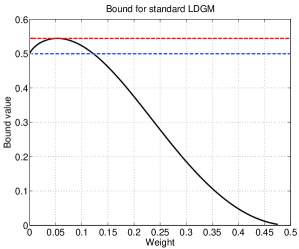
Figure 2: Plot of the function $U(v;D,\gamma_{\operatorname{t}})$ for $D=0.11$ and $\gamma_{\operatorname{t}}=4$. For $v=0$, we have $U(0;D;\gamma_{\operatorname{t}})=1-H_{b}\left(D\right)$, so that the upper bound (4) is always above the Shannon bound. The value $\max_{v\in[0,1]}U(v;D,\gamma_{\operatorname{t}})$ determines the excess rate required beyond the Shannon bound to achieve distortion $D$.

We begin by stating our main results on the rate-distortion performance of LDGM codes. For $\delta\in(0,1)$ and $D,u\in[0,\frac{1}{2}]$, define $\lambda^{*}(\delta,D,u)=\min\{0,\log\rho^{*}(\delta,D,u)\}$, where $\rho^{*}$ is the unique positive root of the quadratic equation $Ax^{2}+Bx+C$ with coefficients

$$A = \delta\,(1-\delta)\,(1-D)$$ (2a)

$$B = u(1-\delta)^{2}+(1-u)\delta^{2}-D\left[\delta^{2}+(1-\delta)^{2}\right].$$ (2b)

$$C = -D\delta(1-\delta).$$ (2c)

For $\delta=0$, we set $\lambda^{*}(0,D,u)=0$. Next define the function $F[D,\delta]$ in a variational manner as follows

$$\max_{u\in[0,D]}\biggr{\{}H_{b}\left(u\right)-H_{b}\left(D\right)+u\log\left[(1-\delta)e^{\lambda^{*}(\delta,D,u)}+\delta\right]\\ +(1-u)\log\left[\delta e^{\lambda^{*}(\delta,D,u)}+(1-\delta)\right]-D\,\lambda^{*}(\delta,D,u)\biggr{\}}.$$ (3)

With these definitions, we have:

Theorem 1.

The rate-distortion function of the $\gamma_{\operatorname{t}}$-regular ensemble is upper bounded by

$$R_{\operatorname{up}}(D;\gamma_{\operatorname{t}}):\,=\max_{v\in[0,1]}\left\{\frac{1-H_{b}\left(D\right)+F\left[D;\delta(v;\gamma_{\operatorname{t}})\right]}{1-H_{b}\left(v\right)}\right\}.\quad$$ (4)

To provide some intuition for the behavior of the function $U(v;D,\gamma_{\operatorname{t}}):\,=\frac{1-H_{b}\left(D\right)+F\left[D;\delta(v;\gamma_{\operatorname{t}})\right]}{1-H_{b}\left(v\right)}$ that determines the bound (4), Figure 2 provides a plot for the case $D=0.11$ and $\gamma_{\operatorname{t}}=4$. For $v=0$, it can be seen that $F\left[D;\delta(0;\gamma_{\operatorname{t}})\right]=0$, so that the $U(0;D,\gamma_{\operatorname{t}})=1-H_{b}\left(D\right)$, implying that the upper bound is always larger than the Shannon lower bound.

By determining the maximum (4) for a range of rates and degrees $\gamma_{\operatorname{t}}$, we can trace out parametric upper bounds on the rate-distortion function. Figure 3 provides plots of the bound (4) on the rate-distortion function for $\gamma_{\operatorname{t}}\in\{3,4,6\}$. Also shown is the Shannon curve $\mathrm{R}(D)=1-H_{b}\left(D\right)$, which is a lower bound for any construction. Finally, an important special case of Theorem 1 is the limit of zero distortion ($D=0$), in which case the rate-distortion function corresponds to the satisfiability threshold. In this case, we recover as a corollary the following result previously established by Creignou et al. [6]:

Corollary 1.

The random $\gamma_{\operatorname{t}}$-XORSAT satisfiability threshold is lower bounded by $\alpha^{*}(\gamma_{\operatorname{t}}):\,=\frac{1}{R_{\operatorname{up}}(0;\gamma_{\operatorname{t}})}$, where

$$R_{\operatorname{up}}(0;\gamma_{\operatorname{t}}) = \max_{v\in[0,\frac{1}{2}]}\frac{1+\log\left[1-\delta(v;\gamma_{\operatorname{t}})\right]}{1-H_{b}\left(v\right)}$$ (5)

This special case reveals that our upper bounds are not sharp, as the bounds (5) are known to be loose for the $D=0$ case. Indeed, several researchers [14, 5, 7] have derived the exact threshold values for the XORSAT problem. However, the looseness in the bound (5) rapidly vanishes as $\gamma_{\operatorname{t}}$ increases. As an illustration, for $\gamma_{\operatorname{t}}=3$, we have $\alpha^{*}(3)=0.88949$ in contrast to the exact threshold $c^{*}(3)=0.91794$, whereas for $\gamma_{\operatorname{t}}=6$, we have $\alpha^{*}(6)=0.99623$ in contrast to the exact threshold $c^{*}(6)=0.99738$.

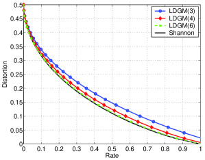
Figure 3: The Shannon rate-distortion function $\mathrm{R}(D)=1-H_{b}\left(D\right)$ provides a lower bound on any construction. Plots of the upper bound (4) for LDGM ensembles with $\gamma_{\operatorname{t}}\in\{3,4,6\}.$

II-C Proof of Theorem 1

The remainder of this section is devoted to proving the previous result. Our proof exploits Shepp’s second moment method, which is a standard tool in satisfiability analysis:

Lemma 2.

For any positive integer valued random variable $\mathssf{z}$, we have $\mathbb{P}[\mathssf{z}>0]\geq\frac{\mathrm{E}[\mathssf{z}]^{2}}{\mathrm{E}[\mathssf{z}^{2}]}$.

Given an LDGM code $\mathbf{{C}}$ of rate $\mathrm{R}=\frac{m}{n}>0$, let $N=2^{n\mathrm{R}}$ be the total number of codewords. For a given sequence $\mathbf{s}\in\{0,1\}^{n}$, define for each codeword $i=1,\ldots,N$ an indicator variable $x_{i}(\mathbf{{C}},\mathbf{s},D)$ for the event that codeword $i$ is within Hamming distance $Dn$ of the source sequence $\mathbf{s}$. Thus, the quantity

$$z\left(\mathbf{{C}},\mathbf{s},D\right) = \sum_{i=1}^{N}x_{i}(\mathbf{{C}},\mathbf{s},D)$$ (6)

is the total number of codewords that are distortion $D$-optimal. In order to apply apply the second moment bound (Lemma 2) to this random variable, we need to compute the first and second moments. Here we will be taking expectations over both the source sequence $\mathbf{s}\sim\operatorname{Ber}(\frac{1}{2})$ and the choice of random code $\mathbf{{C}}$ from the $\gamma_{\operatorname{t}}$-regular ensemble. In the following analysis, we will provide conditions such that

$$\log\mathbb{E}[z\left(\mathbf{{C}},\mathbf{s},D\right)]^{2}-\log\mathbb{E}[z\left(\mathbf{{C}},\mathbf{s},D\right)^{2}] > -\log q(n),$$

where $q(n)$ is a polynomial function of $n$. It can be shown [11] using martingale arguments that such a statement is sufficient to establish that the expected distortion is less than $D$. Consequently, we analyze normalized log probabilities (i.e., $\frac{1}{n}\log\mathbb{E}[z\left(\mathbf{{C}},\mathbf{s},D\right)]$), and write $o(1)$ to capture terms of the form $\frac{\log q(n)}{n}$. The first moment is straightforward to bound using standard results:

Lemma 3.

The first moment is sandwiched as

$$\mathbb{E}[z\left(\mathbf{{C}},\mathbf{s},D\right)] \geq \frac{1}{n+1}2^{n\left[\mathrm{R}-(1-H_{b}\left(D\right))\right]}.$$ (7a)

$$\mathbb{E}[z\left(\mathbf{{C}},\mathbf{s},D\right)] \leq (n+1)\;2^{n\left[\mathrm{R}-(1-H_{b}\left(D\right))\right]}.$$ (7b)

We also make use of the following alternative expression for the second moment (see [11] for a proof):

Lemma 4.

The second moment can $\mathrm{E}[\mathssf{z}(D)^{2}]$ can be decomposed as

$$E[\mathssf{z}(D)]+E[\mathssf{z}(D)]\;\sum_{j\neq 0}\mathbb{P}[\mathssf{x}_{j}(D)=1\mid\mathssf{x}_{0}(D)=1].$$ (8)

Particularly important in our analysis is the following lemma, which provides a large deviations upper bound on the conditional probability in equation (8):

Lemma 5.

Conditioned on the event that codeword $j$ has a fraction $vn$ ones, we have

$$\frac{1}{n}\log\mathbb{P}\left[\mathssf{x}_{j}(D)=1\mid\mathssf{x}_{0}(D)=1\right] \leq F\left[D;\delta(v;\gamma_{\operatorname{t}})\right]+o(1),\quad$$

where the function $F$ is defined in equation (3).

Proof:  We can reformulate the probability on the LHS as follows. Let $\mathssf{T}$ be a discrete variable with distribution

$$\mathbb{P}(\mathssf{T}=t) = \frac{{n\choose t}}{\sum_{s=0}^{Dn}{n\choose s}}\qquad\mbox{for $t=0,1,\ldots,Dn$},$$

representing the (random) number of $1$s in the source sequence $\mathbf{s}$. Let $\mathssf{Y}_{i}$ and $\mathssf{W}_{j}$ denote Bernoulli random variables with parameters $1-\delta(v;\gamma_{\operatorname{t}})$ and $\delta(v;\gamma_{\operatorname{t}})$ respectively. With this set-up, conditioned on codeword $j$ having a fraction $vn$ ones, the probability $\mathbb{P}[\mathssf{x}_{j}(D)=1\mid\mathssf{x}_{0}(D)=1]$ is equivalent to the probability that the random variable

$$\mathssf{U} :\,= \sum_{i=1}{T}\mathssf{Y}_{j}+\sum_{j=1}^{n-\mathssf{T}}\mathssf{W}_{j}$$ (9)

is less than $Dn$. To bound this probability, we use Chernoff’s bound in the form

$$\frac{1}{n}\log\mathbb{P}[\mathssf{U}\leq Dn] \leq \inf_{\lambda<0}\left(\frac{1}{n}\log\mathbb{M}_{\mathssf{U}}(\lambda)-\lambda D\right).$$ (10)

We begin by computing the moment generating function $\mathbb{M}_{\mathssf{U}}$. Taking conditional expectations and using independence, we have

$$\mathbb{M}_{\mathssf{U}}(\lambda) = \sum_{t=0}^{Dn}\mathbb{P}[\mathssf{T}=t]\;\left[\mathbb{M}_{\mathssf{Y}}(\lambda)\right]^{t}\left[\mathbb{M}_{\mathssf{W}}(\lambda)\right]^{n-t}$$

Of interest to us is the exponential behavior of this expression in $n$. Using the standard entropy approximation to the binomial coefficient, we can write $\frac{1}{n}\log\mathbb{M}_{\mathssf{U}}(\lambda)$ as

$$\frac{1}{n}\log\biggr{\{}\sum_{t=0}^{Dn}\exp\big{[}n\big{\{}H_{b}\left(\frac{t}{n}\right)-H_{b}\left(D\right)+\frac{t}{n}\log\mathbb{M}_{\mathssf{Y}}(\lambda)\\ +\left(1-\frac{t}{n}\right)\log\mathbb{M}_{\mathssf{W}}(\lambda)\big{\}}\big{]}\biggr{\}}+o(1)$$

where the cumulant generating functions have the form

$$\log\mathbb{M}_{\mathssf{Y}}(\lambda) = \log\left[(1-\delta)e^{\lambda}+\delta\right].$$ (11a)

$$\log\mathbb{M}_{\mathssf{W}}(\lambda) = \log\left[(1-\delta)+\delta e^{\lambda}\right].$$ (11b)

Note that the exponential behavior of the Chernoff bound (10) is determined by $\max_{u\in[0,D]}G(u;\lambda)$ where

$$G(u;\lambda):\,=H_{b}\left(u\right)-H_{b}\left(D\right)+u\log\mathbb{M}_{\mathssf{Y}}(\lambda)\\ +(1-u)\log\mathbb{M}_{\mathssf{W}}(\lambda)-\lambda D.$$

Since cumulant generating functions are strictly convex, we are guaranteed that $G$ is strictly convex in $\lambda$; similarly, it can be seen that $G$ is strictly concave in $u$. Moreover, for any $D>0$ and $\delta\in(0,1)$, we have $G(u;\lambda)\rightarrow+\infty$ as $\lambda\rightarrow-\infty$. Thus, by standard min-max results [9], we can interchange the order of minimization (over $\lambda<0$) and maximization (over $u\in[0,D]$). Taking derivatives with respect to $\lambda$ to find the minimum, we find that $\frac{\partial F}{\partial\lambda}=0$ is equivalent to

$$u\frac{(1-\delta)\exp(\lambda)}{(1-\delta)\exp(\lambda)+\delta}+(1-u)\frac{\delta\exp(\lambda)}{(1-\delta)+\delta\exp(\lambda)}-D\,=\,0.\quad$$

This is a quadratic equation in $\exp(\lambda)$ with coefficients specified in equation (2a); the unique positive root is $\rho^{*}$ as defined. Finally, from the Chernoff bound (10), we have

$$\frac{1}{n}\log\mathbb{P}[\mathssf{U}\leq nD] \leq \sup_{u\in[0,D]}G(u;\lambda^{*}(u;D)).$$

Recognizing that $F[D,\delta]=\sup_{u\in[0,D]}G(u;\lambda^{*}(u;D))$ completes the proof of the lemma. ∎

We are now ready to complete the proof of the theorem. First of all, by combining Lemmas 3 and  5, we can upper bound $\frac{1}{n}\log E[\mathssf{z}(D)]\;\sum_{j\neq 0}\mathbb{P}[\mathssf{x}_{j}(D)=1\mid\mathssf{x}_{0}(D)=1]$ by

$$\mathrm{R}\left(1-H_{b}\left(D\right)\right)+\max_{v\in[0,1]}\left\{\mathrm{R}H_{b}\left(v\right)+F[D,\delta(v;\gamma_{\operatorname{t}})]\right\}.$$

Combining with Lemma 4, we obtain that $\frac{1}{n}\log E[\mathssf{z}(D)^{2}]$ is upper bounded by

$$\mathrm{R}\left(1-H_{b}\left(D\right)\right)+\max_{v\in[0,1]}\left\{\mathrm{R}H_{b}\left(v\right)+F[D,\delta(v;\gamma_{\operatorname{t}})]\right\}+o(1).$$

Now plugging this bound into the second moment bound (Lemma 2) and using Lemma 3, we obtain that $\frac{1}{n}\log\mathbb{P}[\mathssf{z}(D)>0]$ is lower bounded by

$$\mathrm{R}\left(1-H_{b}\left(D\right)\right)-\max_{v\in[0,1]}\left\{\mathrm{R}H_{b}\left(v\right)+F[D,\delta(v;\gamma_{\operatorname{t}})]\right\}+o(1).$$

The probability of finding a $D$-optimal word will not vanish exponentially fast as long as this quantity stays non-negative; with some simple algebra, this condition is equivalent to the bound

$$\mathrm{R} \geq \max_{v\in[0,1]}\frac{1-H_{b}\left(D\right)+F[D,\delta(v;\gamma_{\operatorname{t}})]}{1-H_{b}\left(v\right)}.$$ (12)

Therefore, the true rate distortion function must be smaller than the RHS of this equation, thereby completing the proof of the theorem. ∎

II-D Proof of Corollary 1

To prove the corollary with $D=0$, we note that equation (9) now entails evaluating the probability that $\sum_{j=1}^{n}\mathssf{W}_{j}=0$, where the $\mathssf{W}_{j}$ are i.i.d. $\operatorname{Ber}(\delta(v;\gamma_{\operatorname{t}}))$ variables. By Sanov’s theorem, the error exponent (i.e., $F$) in this case is simply $D\left(0||\delta(v;\gamma_{\operatorname{t}})\right)=\log(1-\delta(v;\gamma_{\operatorname{t}}))$. Substituting this into equation (4) and using the fact that $H_{b}\left(0\right)=0$ yields the result.

\psfrag{#k#}{$k$}\psfrag{#m#}{$m$}\psfrag{#topdeg#}{$\gamma_{\operatorname{t}}$}\psfrag{#vdeg#}{$\gamma_{v}$}\psfrag{#cdeg#}{$\gamma_{c}$}\psfrag{#n#}{$n$}\psfrag{#G#}{$\mathbf{{G}}$}\psfrag{#H1#}{$\mathbf{{H}}_{1}$}\psfrag{#H2#}{$\mathbf{{H}}_{2}$}\includegraphics[keepaspectratio,width=221.14381pt]{StandConstruct.eps}

Figure 4: Illustration of compound LDGM and LDPC code construction. The top section consists of an $(n,m)$ LDGM code with generator matrix $\mathbf{{G}}$ and constant check degrees $\gamma_{\operatorname{t}}=4$; its rate is $R(\mathbf{{G}})=\frac{m}{n}$. The bottom section consists of a $(m,k)$ LDPC codes with degree $(\gamma_{v},\gamma_{c})=(2,4)$, described by parity check matrix $\mathbf{{H}}$ and with rate $R(\mathbf{{H}})=1-\frac{k}{m}$.

III Compound Constructions

In this section, we describe a compound construction, discussed in our previous work [11] in which an LDGM code is concatenated with an LDPC code. By contrast with the standard LDGM construction, finite degrees suffice to saturate the rate-distortion bound. The compound code construction is illustrated in Fig. 4; it is defined by a factor graph with three layers, and consists of an LDGM code with generator matrix $\mathbf{{G}}$ and an LDPC code with parity check matrix $\mathbf{{H}}$. Note that a sequence $\mathbf{y}\in\{0,1\}^{n}$ is a codeword of this joint LDPC/LDGM construction if and only if there exists an information sequence $\mathbf{z}\in\{0,1\}^{m}$ such that (a) $\mathbf{z}^{\prime}\mathbf{{G}}=\mathbf{y}^{\prime}$, and (b) $\mathbf{{H}}\mathbf{z}=0$ (where all operations are in modulo two arithmetic).

The major deficit of LDGM codes—from the point of view of both source and channel coding—is that they contain large numbers of poorly separated codewords. Herein lies the motivation for adding the bottom LDPC precode: it serves to push apart the valid information bit sequences $\mathbf{z}\in\{0,1\}^{m}$, thereby spreading apart the associated sequences $\mathbf{z}^{\prime}\mathbf{{G}}$ that are codewords in the joint LDGM/LDPC construction. To formalize this intuition, a proof similar to that of Theorem 1 establishes the following

Theorem 2.

The rate-distortion function of $\gamma_{\operatorname{t}}$-regular LDGM/LDPC compound construction (with asymptotic LDPC weight enumerator $\mathcal{A}(v)$) is upper bounded by $R_{\operatorname{com}}(D;\gamma_{\operatorname{t}}):\,=\max_{v\in[0,1]}V(v;D,\gamma_{\operatorname{t}})$, where

$$V(v;D,\gamma_{\operatorname{t}}):\,=\left\{\frac{1-H_{b}\left(D\right)+F\left[D;\delta(v;\gamma_{\operatorname{t}})\right]}{1-\mathcal{A}(v)\big{/}R(\mathbf{{H}})}\right\}.$$ (13)

Note that this statement includes Theorem 1 as a special case, in which $R(\mathbf{{H}})=1$ and $\mathcal{A}(v)=H_{b}\left(v\right)$. Of interest to us here is that these compound constructions (with $R(\mathbf{{H}})<1$) can saturate the rate-distortion bound with finite degrees. The key is that with suitable choice of LDPC degrees, we can ensure that $\mathcal{A}(v)$ is negative in a region around zero, which prevents the overshooting phenomenon illustrated in Figure 2. More specifically, Figure 5 illustrates the analogous plot for a joint LDGM/LDPC construction with $\gamma_{\operatorname{t}}=4$, LDPC degrees $(\gamma_{v},\gamma_{c})=(4,8)$, rates $R(\mathbf{{G}})=1$ and $R(\mathbf{{H}})=0.5$, and distortion $D=0.11$.

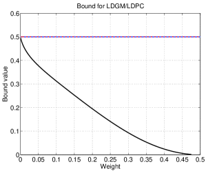
Figure 5: Plot of the function $V(v;D,\gamma_{\operatorname{t}})$ for $\gamma_{\operatorname{t}}=4$, a regular LDPC with degrees $(\gamma_{v},\gamma_{c})=(4,8)$, rates $R(\mathbf{{G}})=1$ and $R(\mathbf{{H}})=0.5$, and distortion $D=0.11$. This function remains below $R=0.5$ for all $v$, so that the code saturates the Shannon lower bound.

Notice how this curve remains below $R=0.5$ for all $v\in[0,0.5]$, demonstrating that the upper bound (13) meets the Shannon lower bound.

IV Discussion

In concurrent work [12], we have shown that the joint LDGM/LDPC construction in Figure 4 generates good nested constructions (i.e., a good channel code can be partitioned into good source codes, and vice versa), which can be shown to saturate the Wyner-Ziv and Gelfand-Pinsker bounds. We have also shown [17] that message-passing algorithms based on survey propagation [3], when applied to LDGM codes with suitable degree distributions, yield rate-distortion trade-offs very close to the Shannon bound. It remains to explore variants of such message-passing algorithms for the compound construction, and problems of coding with side information.

References

- [1] J. Chou, S. S. Pradhan, and K. Ramchandran. Turbo coded trellis-based constructions for data embedding: Channel coding with side information. In Proceedings of the Asilomar Conference, 2001.
- [2] J. Chou, S. S. Pradhan, and K. Ramchandran. Turbo and trellis-based constructions for source coding with side information. In Data Compression Conference (DCC), 2003.
- [3] S. Ciliberti and M. Mézard. The theoretical capacity of the parity source coder. Technical report, August 2005. arXiv:cond-mat/0506652.
- [4] S. Ciliberti, M. Mézard, and R. Zecchina. Message-passing algorithms for non-linear nodes and data compression. Technical report, November 2005. arXiv:cond-mat/0508723.
- [5] S. Cocco, O. Dubois, J. Mandler, and R. Monasson. Rigorous decimation-based construction of ground pure states. Physical Review Letters, 90(4), January 2003.
- [6] N. Creignou, H. Daude, and O. Dubois. Approximating the satisfiability threshold of random -XOR formulas. Combinatorics, Probability and Computing, 12:113–126, 2003.
- [7] O. Dubois and J. Mandler. The 3-XORSAT threshold. In Proc. 43rd Symp. FOCS, pages 769–778, 2002.
- [8] U. Erez and S. ten Brink. A close-to-capacity dirty paper coding scheme. IEEE Trans. Info. Theory, 51(10):3417–3432, 2005.
- [9] J. Hiriart-Urruty and C. Lemaréchal. Convex analysis and minimization algorithms, volume 1. Springer-Verlag, New York, 1993.
- [10] M. W. Marcellin and T. R. Fischer. Trellis coded quantization of memoryless and Gauss-Markov sources. IEEE Trans. Comm., 38(1):82–93, 1990.
- [11] E. Martinian and M. J. Wainwright. Low density codes achieve the rate-distortion bound. In Data Compression Conference, volume 1, page To appear, 2006.
- [12] E. Martinian and M. J. Wainwright. Low density codes can achieve the Wyner-Ziv and Gelfand-Pinsker bounds. Submitted to ISIT, 2006.
- [13] E. Martinian and J. S. Yedidia. Iterative quantization using codes on graphs. In Allerton Conference on Communication, Control, and Computing, Monticello, IL, October 2003.
- [14] M. Mézard, F. Ricci-Tersenghi, and R. Zecchina. Alternative solutions to diluted p-spin models and XORSAT problems. Jour. of Statistical Physics, 111:105, 2002.
- [15] T. Murayama. Thouless-Anderson-Palmer approach for lossy compression. Physical Review E, 69:035105(1)–035105(4), 2004.
- [16] T. J. Richardson and R. L. Urbanke. The capacity of low-density parity-check codes under message-passing decoding. IEEE Trans. Info. Theory, 47(2):599–618, February 2001.
- [17] M. J. Wainwright and E. Maneva. Lossy source coding via message-passing and decimation over generalized codewords of LDGM codes. In Proc. Int. Symp. Info. Theory, September 2005.
- [18] Y. Yang, V. Stankovic, Z. Xiong, and W. Zhao. On multiterminal source code design. In Data Compression Conference, 2005.