Why neighbor-joining works

Abstract.

We show that the neighbor-joining algorithm is a robust quartet method for constructing trees from distances. This leads to a new performance guarantee that contains Atteson’s optimal radius bound as a special case and explains many cases where neighbor-joining is successful even when Atteson’s criterion is not satisfied. We also provide a proof for Atteson’s conjecture on the optimal edge radius of the neighbor-joining algorithm. The strong performance guarantees we provide also hold for the quadratic time fast neighbor-joining algorithm, thus providing a theoretical basis for inferring very large phylogenies with neighbor-joining.

1. Introduction

The widely used neighbor-joining algorithm [24] has been extensively analyzed and compared to other tree construction methods. Previous studies have mostly focused on empirical testing of neighbor-joining. Examples include the comparison of neighbor-joining with quartet [15] and maximum likelihood [14] methods, comprehensive comparisons of multiple programs [13, 16], and detailed testing of the limits of the neighbor-joining algorithm [17]. These studies have concluded that neighbor-joining is effective for many problems, and have recommended the algorithm. For example, in [15] it is remarked that “quartet-based methods are much less accurate than the simple and efficient method of neighbor-joining”. In a recent study, Tamura et al. [29] conclude that there are “bright prospects for the application of the NJ and related methods in inferring large phylogenies.”

Furthermore, new methods are now almost always compared with neighbor-joining to establish an improvement in performance [2, 8, 11, 19, 20, 23, 27]. In other words, neighbor-joining has become the standard by which new phylogenetic algorithms are compared, and continues to surface as an effective candidate method for constructing large phylogenies. This is remarkable, considering the simplicity of the neighbor-joining algorithm. We begin with a review of the neighbor-joining algorithm and a very brief description of basic concepts involved. The definitions and notation are based on [26]. The reader unfamiliar with the concepts described below should consult this reference for full details.

Throughout the text a phylogenetic $X$-tree $T$ denotes a binary tree describing the evolutionary relationships between a set of taxa $X$, which label the leaves of the tree. We will also use the term phylogenetic tree when the set $X$ is clear from the context. A cherry of $T$ is a pair of leaves (or taxa) $(i,j)\in{X\choose 2}$ such that the path from $i$ to $j$ in $T$ has length exactly 2 (i.e. $i,j$ have a common “parent” in $T$).

A split $A|B$ of $X$ is a bipartition $X=A\cup B$ and $A\cap B=\emptyset$. In general we will use splits of $X$ induced by removing an internal edge of $T$ (which will result in creating two disconnected trees, one with leaf set $A$ and the other with leaf set $B$).

A dissimilarity map on $X$ is a map $\delta:X\times X\rightarrow\mathbb{R}$ satisfying $\delta(x,y)=\delta(y,x)$, $\delta(x,y)\geq 0$ and $\delta(x,x)=0$ for all $x,y\in X$. A tree metric, or an additive dissimilarity map, is a dissimilarity map $\delta$ for which there exists a tree $T$ with edge lengths $l:E(T)\rightarrow(0,\infty)$ such that $\delta(i,j)=\sum_{e\in P(i,j)}l(e)$ where $P(i,j)$ is the set of edges in $E(T)$ on the path from $i$ to $j$ in $T$. We note that for an additive dissimilarity map, the tree topology and edge lengths $l$ are uniquely defined.

We are now ready to give the full description of neighbor-joining:

1. Given a set of taxa $X$ and a dissimilarity map $\delta:X\times X\rightarrow{\mathbb{R}}$ (this is a map that satisfies $\delta(i,j)=\delta(j,i)$ and $\delta(i,i)=0$), compute the Q-criterion for $\delta$

   $$Q_{\delta}(i,j)=\delta(i,j)-\frac{1}{n-2}\left(\sum_{k\neq i}\delta(i,k)+\sum_{k\neq j}\delta(j,k)\right).$$

   Then select a pair $a,b$ that minimize $Q_{\delta}$ as motivated by the following theorem:

   Theorem 1 (Saitou-Nei [24] and Studier-Keppler [28]).

   Let $\delta_{T}$ be the tree metric corresponding to the tree $T$. The pair $a,b$ that minimizes $Q_{\delta_{T}}(i,j)$ is a cherry in the tree.

2. If there are more than three taxa, replace the putative cherry $a$ and $b$ with a leaf $j_{ab}$, and construct a new dissimilarity map where $\delta(i,j_{ab})=\frac{1}{2}(\delta(i,a)+\delta(i,b))$. This is called the reduction step.

3. Repeat until there are three taxa.

Although the $Q$-criterion is easy to compute, the formula seems, at first glance, somewhat contrived and mysterious. However, the formulation of the $Q$-criterion is not accidental and has many useful properties. For example, it is linear in the distances, is permutation equivariant (the input order of the taxa don’t matter), and it is consistent, i.e., it correctly finds the tree corresponding to a tree metric. Bryant [3] has shown that the $Q$-criterion is in fact the unique selection criterion satisfying these properties. Gascuel and Steel [12] in an excellent review, provide a very precise mathematical answer to “what does neighbor-joining do?”, via a proof that neighbor-joining is a greedy algorithm which “decreases the whole tree length” as computed by Pauplin’s formula [5, 21].

These results motivate the neighbor-joining algorithm, but they do not offer any insight into its performance with dissimilarity maps that are not tree metrics. More importantly, they do not address the central question of the behavior of neighbor-joining on dissimilarity maps that arise from maximum likelihood estimation of distances between sequences in multiple alignments. There is one result that addresses precisely these issues:

Theorem 2 (Atteson [1]).

Neighbor-joining has $l_{\infty}$ radius $\frac{1}{2}$.

This means that if the distance estimates are at most half the minimal edge length of the tree away from their true value then neighbor-joining will reconstruct the correct tree. Atteson’s theorem shows that neighbor-joining is statistically consistent. Informally, this means that neighbor-joining reconstructs the correct tree from dissimilarity maps estimated from sufficiently long multiple alignments. This has been a widely used justification for the observed success of neighbor-joining, and is regarded as the definitive explanation for “when does neighbor-joining work?” [12].

However, as noted in [18], Atteson’s condition frequently fails to be satisfied even when neighbor-joining is successful. This is also remarked on in [6]: “In practice, most distances are far from being nearly additive [satisfying Atteson’s condition]. Thus, although important, optimal reconstruction radius is not sufficient for an algorithm to be useful in practice.” Our main result is an explanation of why neighbor-joining is useful in practice. We obtain our results using a new consistency theorem (Theorem 16 in Section 4). Roughly speaking, our theorem states that neighbor-joining is successful (globally) when it works correctly (locally) for the quartets in the tree. Thus, Theorem 16 provides a crucial link between neighbor-joining and quartet methods, a connection that is first developed in Section 3. We also show that Atteson’s theorem is a special case of our theorem.

In Section 5 we present a proof of Atteson’s conjecture on the optimal edge radius of neighbor-joining. For a dissimilarity map $\delta$ whose $l_{\infty}$ distance to a tree metric $\delta_{T}$ is less than $\frac{\epsilon}{4}$, we prove that the output $T^{\prime}$ of neighbor-joining applied to $\delta$ will contain all edges of $T$ of length at least $\epsilon$, i.e., neighbor-joining has $l_{\infty}$ edge radius $\frac{1}{4}$. We say that $T^{\prime}$ contains the edge $e$ if there exists an edge $e^{\prime}\in T^{\prime}$ such that the split of the taxa induced by removing $e^{\prime}$ from $T^{\prime}$ is the same as that induced by removing $e$ from $T$. This result is tight, as [1] provides a counterexample for edge radius larger than $\frac{1}{4}$. The methods we employ for this result are virtually the same as the ones used in the proof of Theorem 16, although the proof is non-constructive and based on an averaging argument. We conclude with a simulation study that establishes the practical significance of our theorems in Section 6.

2. The shifting lemma

In this section we provide a few preliminary observations that are necessary for our results. We begin by reviewing a lemma from [10], namely that there is an alternative to the reduction step (2) in the neighbor joining algorithm. Condition (2’): if there are more than three taxa, replace the putative cherry $a$ and $b$ with a leaf $j_{ab}$, and construct a new dissimilarity map where $\delta(i,j_{ab})=\frac{1}{2}(\delta(i,a)+\delta(i,b)-\delta(a,b))$.

Notice that the only difference between (2) and (2’) consists of addition of the $-\delta(a,b)$ term. On a tree metric, the first version of the algorithm corresponds to replacing a cherry by a single node whose distance to the rest of the tree is the average of the distances of the two collapsed nodes. In the second version, the reduction step is equivalent with replacing the cherry by its “root”, i.e., the point where the path between the cherry nodes connects to the rest of the tree.

Definition 3.

We say the dissimilarity map $\delta^{\prime}$ is a shift of $\delta$ if and only if there exists a fixed $\epsilon$ and a distinguished taxon $a$, such that $\delta^{\prime}(a,x)=\delta(a,x)+\epsilon$ for all $x\neq a$ and $\delta^{\prime}(x,y)=\delta(x,y)$ for all $x,y\neq a$.

Lemma 4 (The shifting lemma [10]).

Shifting does not affect the outcome of neighbor-joining.

Proof: This follows from the observation that shifting by $\epsilon$ around $a$ changes the value of $Q(x,y)$ by exactly $-2\epsilon$, for all pairs $x,y$. Moreover, the result of collapsing taxa $x,y$ in the shifted dissimilarity map is the same as the result of collapsing the same taxa in the initial dissimilarity map, or an $\epsilon$ shift of it. By these two observations, at each step neighbor-joining will collapse the same pairs as before the shift. ∎

Corollary 5.

The two versions of neighbor-joining are equivalent: they produce trees with the same topology.

Proof: Collapsing $x,y$ by the second reduction method gives a dissimilarity map that is a $\frac{\delta(x,y)}{2}$-shift of the one produced by collapsing by the first type of reduction step. ∎

It is important to notice that the operation of shifting a real tree metric $\delta_{T}$ by $\epsilon$ around taxon $a$ corresponds exactly to modifying the length of the leaf edge of $T$ corresponding to $a$ by exactly $\epsilon$. So in effect we can allow negative leaf edges since shifting around all leaves by a large enough constant will make them positive, while the outcome of the algorithm is the same. Of course, the statement of our edge radius results does not make sense in the case of negative edge lengths. However, the only negative edges are the leaf edges, and in that case the statements we make are vacuous. They hold trivially since neighbor-joining reconstructs the bipartition consisting of one taxon vs. the rest of the taxa set correctly, regardless of the input.

In the remainder of the paper, by a tree metric we will mean a shift of a tree metric, i.e. a metric corresponding to a tree where leaf edges are allowed to be negative.

3. Quartets and neighbor-joining

We now show that for four taxa, neighbor joining is equivalent to the four point method [7]. We will use the notation $(ij:kl)$ to denote the tree topology on the set $\{i,j,k,l\}$ where the pairs $(i,j)$ and $(k,l)$ form cherries separated by a middle edge. When $i,j,k,l$ are leaves (internal or external) of a tree $T$, we will say that $(ij:kl)$ is a quartet of $T$ if the topology induced by $T$ on the four nodes is that indicated by $(ij:kl)$ .

Proposition 6.

Let $X=\{i,j,k,l\}$ and $\delta:X\times X\rightarrow{\mathbb{R}}$ be a dissimilarity map. The neighbor-joining algorithm will return the tree $(ij:kl)$ where $\delta(i,j)+\delta(k,l)\leq min(\delta(i,k)+\delta(j,l),\delta(i,l)+\delta(j,k))$.

This result can be easily derived using the $Q$-criterion, but we prefer to motivate it using an alternative formulation of the neighbor-joining criterion formulated in [10].

For a dissimilarity map $\delta$, let

$$w_{\delta}(ij:kl)=\frac{1}{2}\left(\delta(i,k)+\delta(i,l)+\delta(j,k)+\delta(j,l)\right)-\delta(i,j)-\delta(k,l).$$

Note that for a quartet $(ij:kl)$ in a tree $T$ with corresponding tree metric $\delta_{T}$, $w_{\delta_{T}}(ij:kl)$ is double the length of the internal edge in the quartet. In [10] this is called a “neighborliness” measurement.

Theorem 7.

If $\delta_{T}$ is the tree metric corresponding to a phylogenetic $X$-tree $T$ and

$$Z_{\delta_{T}}(i,j)=\frac{1}{{n-1\choose 2}}\sum_{(k,l)\in{{X\backslash\{i,j\}}\choose{2}}}w_{\delta_{T}}(ij:kl)$$

then the pair $a,b$ that maximizes $Z_{\delta_{T}}(i,j)$ is a cherry in the tree.

Proof: Let $n=|X|$. The sum in $Z_{\delta_{T}}$ is over unordered pairs of $X-\{i,j\}$. Observe that for any $\delta$

$$Z_{\delta}(i,j)=-L_{\delta}(T)-Q_{\delta}(i,j)$$

where $L_{\delta}(T)=\frac{1}{{n-1\choose 2}}\sum_{x,y\in T}\delta_{T}(x,y)$ does not depend on $i$ or $j$. The theorem now follows directly from Theorem 1. ∎

Although the naive computation of the $Z$-criterion requires quadratic time, the equivalence with the $Q$-criterion shows that each entry in the $Z$-matrix is just a sum of a linear number of distances. One may therefore wonder why the $Z$-criterion is worth mentioning at all. We outline a number of reasons why the $Z$-criterion may be a more natural way to formulate the neighbor-joining selection criterion. For example, note that in the case of four taxa $i,j,k,l$, the $Z$-criterion is just $Z_{\delta}(i,j)=\frac{1}{3}w_{\delta}(ij:kl)$ and Proposition 6 follows immediately from Theorem 7. The $Z$-criterion also highlights the fact that for a tree metric, the neighbor-joining selection criterion does not depend on the length of edges adjacent to leaves. This is remarked on in the proof of the consistency of neighbor-joining in [3]. Furthermore, for a dissimilarity map $\delta$, $Z_{\delta}(i,j)$ is precisely the difference between the balanced minimum length of $\delta$ with respect to the star tree, and the length with respect to the tree containing the cherry $(i,j)$ with the remaining taxa unresolved (see Figure 1 in [12] and the accompanying discussion).

Finally, the $Z$-criterion highlights the connection between neighbor-joining and quartet methods. Recall that the naive quartet method consists of choosing a quartet for each four taxa using the four point method (Proposition 6), and then returning the tree consistent with all the quartets (if such a tree exists). This leads us to

Definition 8.

A dissimilarity map $\delta$ is quartet consistent with a tree $T$ if for every $(ij:kl)\in T$, $w_{\delta}(ij:kl)>max(w_{\delta}(ik:jl),w_{\delta}(il:jk))$.

By definition, the naive quartet method will reconstruct a tree $T$ from a dissimilarity map $\delta$ if $\delta$ is quartet consistent with $T$. We note that this is essentially the same as the ADDTREE method [25], with the minor difference that ADDTREE always outputs a tree, albeit potentially the wrong one if $\delta$ is not quartet consistent with $T$.

In the next section we will prove the following extension of Proposition 6:

Theorem 9.

If $4\leq|X|\leq 7$ and $\delta:X\times X\rightarrow{\mathbb{R}}$ is a dissimilarity map that is quartet consistent with a binary tree $T$ then the neighbor-joining algorithm applied to $\delta$ will construct a tree with the same topology as $T$. Furthermore, if $5\leq|X|\leq 7$ then there exists $\epsilon>0$ such that if $||\tilde{\delta}-\delta||_{\infty}<\epsilon$, neighbor-joining applied to $\tilde{\delta}$ will reconstruct a tree with the same topology as $T$.

As we have pointed out, neighbor-joining is equivalent to the naive quartet method and ADDTREE for $|X|=4$. Theorem 9 states that neighbor-joining is at least as good as the naive quartet method for trees with at most $7$ taxa, and is in fact robust to small changes in the metric.

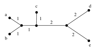
Figure 1. A five leaf tree.

Example 10.

Let $T$ be the 5 leaf tree shown in Figure 1 that corresponds to the tree metric $\delta_{T}$, and consider the distorted dissimilarity map $\delta$

$$\delta_{T}\quad=\quad\bordermatrix{&a&b&c&d&e\cr a&0&2&3&6&6\cr b&2&0&3&6&6\cr c&3&3&0&5&5\cr d&6&6&5&0&4\cr e&6&6&5&4&0\cr},\qquad\delta\quad=\quad\bordermatrix{&a&b&c&d&e\cr a&0&2&3&6&3\cr b&2&0&3&6&6\cr c&3&3&0&5&5\cr d&6&6&5&0&4\cr e&3&6&5&4&0\cr}.$$

Note that $\delta$ is not quartet consistent with $T$, because $\delta(a,e)+\delta(b,c)<\delta(a,b)+\delta(c,e)$. However it is easy to verify that neighbor-joining constructs a tree with the same topology as $T$. The example shows that neighbor-joining can construct the correct tree even when the naive quartet method and ADDTREE fail.

The next example shows that Theorem 9 fails for trees with more than $7$ taxa.

Example 11.

Let $T$ be the 8 leaf tree shown in Figure 2 and let $\delta_{T}$ be its corresponding tree metric.

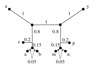
Figure 2. An eight leaf tree.

$$\delta_{T}\quad=\quad\bordermatrix{&x&y&a&b&c&m&n&p\cr x&0&3&2&2&2&3&3&3\cr y&3&0&3&3&3&2&2&2\cr a&2&3&0&0.1&0.4&3&3&3\cr b&2&3&0.1&0&0.4&3&3&3\cr c&2&3&0.4&0.4&0&3&3&3\cr m&3&2&3&3&3&0&0.1&0.4\cr n&3&2&3&3&3&0.1&0&0.4\cr p&3&2&3&3&3&0.4&0.4&0\cr},$$

Consider the distorted dissimilarity map

$$\delta\quad=\quad\bordermatrix{&x&y&a&b&c&m&n&p\cr x&0&2.7&2.6&2.6&2.6&4.4&4.4&4.4\cr y&2.7&0&4.4&4.4&4.4&2.6&2.6&2.6\cr a&2.6&4.4&0&0.1&0.4&2.7&2.7&2.7\cr b&2.6&4.4&0.1&0&0.4&2.7&2.7&2.7\cr c&2.6&4.4&0.4&0.4&0&2.7&2.7&2.7\cr m&4.4&2.6&2.7&2.7&2.7&0&0.1&0.4\cr n&4.4&2.6&2.7&2.7&2.7&0.1&0&0.4\cr p&4.4&2.6&2.7&2.7&2.7&0.4&0.4&0\cr}$$

that is quartet consistent with $T$. It is easy to see that $Q_{\delta}(x,y)=-6.24$, while $Q_{\delta}(a,b)=Q_{\delta}(m,n)=-6.04$. Therefore the function $Q_{\delta}$ is not minimized at one of the cherries of $T$, and the neighbor-joining algorithm applied to $\delta$ outputs a tree different from $T$, in which $x,y$ form a cherry.

Fortunately, there is a single extra condition which ensures that neighbor-joining correctly reconstructs a tree. In what follows we say that a leaf $x$ is interior to a quartet $(ij:kl)$ in a tree $T$ if none of $(ik:xl)$, $(ik:xj)$, $(ix:jl)$, or $(kx:jl)$ are quartets in $T$.

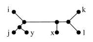
Figure 3. The quartet additivity configuration.

Definition 12.

A dissimilarity map $\delta:X\times X\rightarrow{\mathbb{R}}$ is quartet additive with a tree $T$ if for every $(ij:kl)\in T$ with $x$ interior to $(ij:kl)$, and $y$ not interior to $(ij:kl)$ such that $(ij:xy)$ is not a quartet of $T$, we have $w(kl:xy)>w(ij:xy)$ (see Figure 3).

We conclude with three basic lemmas that are important in the next section. The proofs are left as an exercise for the reader.

Lemma 13.

Quartet consistency and additivity are both invariant with respect to the shifting operation.

Lemma 14 (Spectator Lemma).

For any $a,b,x,y,t\in X$,

$$2w(ab:xy)=w(tb:xy)+w(at:xy)+w(ab:ty)+w(ab:xt).$$

The Spectator Lemma is used to prove

Lemma 15.

For any $a,b,c,i,j,x,y\in X$,

$$3w(ab:xy)-3w(ac:xy) = w(ab:xc)-w(ac:xb)+w(ab:yc)-w(ac:yb),$$

$$4w(ab:xy)-4w(ij:xy) = w^{*}(ab:x:ij)+w^{*}(ab:y:ij),$$

where $w^{*}(ab:x:ij)=w(ab:ix)+w(ab:jx)-w(ax:ij)-w(bx:ij)$.

4. A consistency theorem for neighbor-joining

Theorem 16.

If $\delta:X\times X\rightarrow{\mathbb{R}}$ is quartet consistent and quartet additive with a tree $T$, then neighbor-joining applied to $\delta$ will construct a tree with the same topology as $T$.

The proof of the theorem consists of two main parts. First, we show that when the reduction step collapses a pair of taxa $(x,y)$ which form a cherry in $T$, then the dissimilarity metric given by reducing $\delta$ is quartet consistent and additive with the tree $T^{\prime}$ obtained by clipping off the cherry $(x,y)$ and labeling its former root (now a leaf) with the new taxon thus created in the reduction step. In other words, the node obtained by collapsing $(x,y)$ in $\delta$ is assigned to the location of the common ancestor of $x$ and $y$ in the true tree $T$. Note that this only makes sense when $x$ and $y$ do indeed form a cherry, as this is the only case in which their common ancestor is well defined. The second part of the inductive proof is showing that given $\delta$ quartet consistent and quartet additive with a tree $T$, the optimal pair for the reduction step is guaranteed to form a cherry in $T$. This clearly completes the inductive argument. We proceed with the first step.

Lemma 17.

Quartet consistency is maintained when reducing a cherry of the reference tree. Formally, given a pair of taxa $x,y\in X$ which form a cherry in $T$, the result of collapsing $(x,y)$ in $\delta$ is quartet consistent with the topology given by deleting the leaf edges leading to $x$ and $y$ in $T$ and assigning the new member of the set of taxa to the new leaf thus formed in $T$.

Proof: Without loss of generality, we may assume that we are collapsing taxa $x,y$ into taxon $z$ by using the first type of reduction step. For a set $U\subset X$, we let $T|_{U}$ be the topology induced by $T$ on $U$. Note that for $X_{1}=X-\{x\}$ and $X_{2}=X-\{y\}$, the two topologies $T|_{X_{1}}$ and $T|_{X_{2}}$ are isomorphic under the map $f:X_{1}\rightarrow X_{2}$ defined by $f(u)=u$ for $u\neq x,y$ and $f(y)=x$. We furthermore notice that $\delta|_{X_{i}}$ is quartet consistent with $T|_{X_{i}}$ for $i=1,2$ since $\delta$ is quartet consistent with $T$. Therefore $\delta|_{X_{i}}$ will be quartet consistent with $T^{\prime}$ under identifying $y$ or $x$ with $z$. We note again that this property holds if and only if $(x,y)$ form a cherry in $T$.

Now note that the reduced distance metric $\delta^{\prime}$ on the set $X^{\prime}=X-\{x,y\}\cup\{z\}$ is in fact a linear combination of the two dissimilarity maps $\delta|_{X_{1}}$ and $\delta|_{X_{2}}$ under identifying $z$ with $y$ in $X_{1}$ and $x$ in $X_{2}$ (We define the restriction of the dissimilarity map to a subset of its domain in the obvious way).

The last piece of the proof involves noticing that the condition of quartet consistency with respect to a topology $T$ is a set of linear inequalities (defined by $T$), on the values $\delta(i,j)$, or “linear in $\delta$” for short. Concretely, this means that any linear combination of dissimilarity maps that are quartet consistent with a topology $T$ will also be quartet consistent with $T$. As noted above, both $\delta|_{X_{1}}$ and $\delta|_{X_{2}}$ are quartet consistent with $T^{\prime}$, while $\delta^{\prime}$ is a linear combination of the two under the obvious isomorphisms (in fact $\delta^{\prime}$ is the mean of $\delta|_{X_{1}}$ and $\delta|_{X_{2}}$). We conclude that $\delta^{\prime}$ is quartet consistent with $T^{\prime}$. ∎

Lemma 18.

Quartet additivity is maintained when reducing a cherry of the reference tree. Formally, given a pair of taxa $x,y\in X$ which form a cherry in $T$, the result of collapsing $(x,y)$ in $\delta$ is quartet additive with respect to the topology given by deleting the leaf edges leading to $x$ and $y$ in $T$ and assigning the new member of the set of taxa to the new leaf thus formed in $T$.

Proof: We note that quartet additivity is also a property that is linear in $\delta$. The proof proceeds identically with the previous lemma.

Proof of Theorem 16: By the above lemmas, it suffices to prove that at any step, the pair of taxa which maximize the $Z$-criterion form a cherry. We argue by contradiction. Let us consider a pair $\delta,T$ such that $(i,j)$ is a pair of taxa which maximizes $Z_{\delta}$, but does not form a cherry in $T$. Throughout the proof, and in the remainder of the paper, we multiply $Z_{\delta}$ by ${n-1\choose 2}$ to simplify the formulas.

Case 1: Suppose $i$ or $j$ are part of a cherry. Without loss of generality, assume that leaf $i$ forms a cherry with leaf $k\neq j$ and let $X^{\prime}=X-\{i,j,k\}$. Then:

$$Z_{\delta}(i,k)-Z_{\delta}(i,j)=\sum_{\forall x\in X^{\prime}}w(ik:xj)-w(ij:xk)+\sum_{\forall(x,y)\in{X^{\prime}\choose 2}}w(ik:xy)-w(ij:xy).$$

Applying Lemma 15 to the second summand, we have:

$$Z_{\delta}(i,k)-Z_{\delta}(i,j) = \sum_{\forall x\in X^{\prime}}w(ik:xj)-w(ij:xk)$$

$$+\frac{1}{3}\sum_{\forall x,y\in{X^{\prime}\choose 2}}w(ik:xj)-w(ij:xk)+w(ik:yj)-w(ij:yk)$$

$$= \frac{n-1}{3}\sum_{\forall x\in X^{\prime}}w(ik:xj)-w(ij:xk).$$

Since $(ik:xj)$ is a quartet in $T$ for any $x$, by consistency $w(ik:xj)-w(ij:xk)>0$ for all $x$ and therefore $Z_{\delta}(i,k)-Z_{\delta}(i,j)>0$, a contradiction.

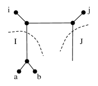
Figure 4. Case 2 in Theorem 16.

Case 2: Neither $i$ nor $j$ are part of a cherry. Then, we have a situation as in Figure 4. Let $I$ be the set of leaves on the subtree nearest $i$ along the path from $i$ to $j$ and, similarly, let $J$ be the set of leaves on the subtree nearest $j$. Without loss of generality, we assume that $|I|\leq|J|$ and let the pair $a,b\in I$ be a cherry in $T$. Let $X^{\prime}=X-\{a,b,i,j\}$. Then

$$Z_{\delta}(a,b)-Z_{\delta}(i,j) = \sum_{x\in X^{\prime}}w(ab:ix)+w(ab:jx)-w(ax:ij)-w(bx:ij)$$

$$+\sum_{x,y\in{X^{\prime}\choose 2}}w(ab:xy)-w(ij:xy).$$

By Lemma 15,

$$Z_{\delta}(a,b)-Z_{\delta}(i,j) = \sum_{x\in X^{\prime}}w^{*}(ab:x:ij)+\frac{1}{4}\sum_{x,y\in{X^{\prime}\choose 2}}w^{*}(ab:x:ij)+w^{*}(ab:y:ij)$$

$$= \frac{n-1}{4}\sum_{x\in X^{\prime}}w^{*}(ab:x:ij)$$

First note that if $x\in X^{\prime}$ is a leaf that is not in $I$ or in $J$ (i.e., the paths from $i$ to $x$ and $j$ to $x$ intersect the path from $i$ to $j$), then $w(ab:xy)>w(ij:xy)$ for any leaf $y$ by quartet consistency. Thus we restrict our attention to the leaves in $I$ and $J$. Let $I^{\prime}=I-\{a,b\}$. Then, since $|I|\leq|J|$, it follows that $|I^{\prime}|\leq|X^{\prime}-I^{\prime}|$ and we choose a subset of $J$ that is the same size as $I^{\prime}$. In particular, there exists $I^{*}\subset J$ such that $|I^{*}|=|I^{\prime}|=P$. Let $I^{\prime}=\{x_{1},...,x_{P}\}$, $I^{*}=\{y_{1},...,y_{P}\}$ and $X^{\prime\prime}=X^{\prime}-I^{\prime}-I^{*}$. Then:

$$\frac{4}{n-1}\left(Z_{\delta}(a,b)-Z_{\delta}(i,j)\right) > \sum_{p=1}^{P}w^{*}(ab:x_{p}:ij)+w^{*}(ab:y_{p}:ij)+\sum_{x\in X^{\prime\prime}}w^{*}(ab:x:ij)$$

$$= 4\sum_{p=1}^{P}w(ab:x_{p}y_{p})-w(ij:x_{p}y_{p})+w(ij:ax)]$$

$$+\frac{2}{3}[w(bi:jx)-w(ij:bx)].$$

Since $(ab:ix),(ai:jx)$ and $(bi:jx)$ are all quartets in $T$, by consistency each term is positive. Therefore $w^{*}(ab:x:ij)>0$ and so $Z_{\delta}(a,b)>Z_{\delta}(i,j)$, a contradiction. ∎

Remark 19.

Theorem 9 follows from the observation that quartet consistency suffices in the proof of Theorem 16 when $4\leq|X|\leq 7$. Details are omitted.

Corollary 20.

Neighbor-joining has $l_{\infty}$ radius of at least $\frac{1}{2}$. Following Atteson’s results from [1] for the reverse inequality, we conclude that neighbor-joining has $l_{\infty}$ radius equal $\frac{1}{2}$.

Proof: It is easy to see that if $\delta_{T}$ is a tree metric and $\delta$ is a metric with $max_{i,j}|\delta_{T}(i,j)-\delta(i,j)|<\frac{1}{2}min_{e\in E(T)}l(e)$ where $l(e)$ is the length of edge $e$ in $T$, then $\delta$ is quartet consistent and quartet additive with $T$. ∎

The next corollary extends the Visibility Lemma from [6]. A taxon $b$ is visible from $a$ with respect to a dissimilarity map $\delta$ if

$$b=argmax_{x\neq a}Z_{\delta}(a,x).$$

Corollary 21.

If $\delta$ is quartet consistent with a tree T and $(a,b)$ is a cherry of $T$, then $b$ is visible from $a$ with respect to $\delta$.

Proof: This follows directly from the first step of the proof of Theorem 16. ∎

The Visibility Lemma is the key to developing a fast neighbor joining algorithm (FNJ) that has optimal run time complexity $O(n^{2})$ [6]. In fact, we can conclude that

Corollary 22.

If $\delta$ is quartet consistent and quartet additive with respect to a tree $T$ then FNJ will reconstruct $T$ from $\delta$ with run time complexity $O(n^{2})$ (which is also the size of the algorithm input).

5. The Edge Radius of the neighbor-joining Algorithm

In this section we prove a strengthening of the following conjecture about the edge radius of the neighbor-joining algorithm:

Conjecture 23 (Atteson [1]).

Let $T$ be a phylogenetic $X$-tree with associated tree metric $\delta_{T}$, and let $e$ be an edge of $T$ of length $l(e)$. If $\delta$ is a dissimilarity map whose $l_{\infty}$ distance to $\delta_{T}$ is less than $\frac{l(e)}{4}$, then neighbor-joining applied to $\delta$ will reconstruct the edge $e$ correctly, i.e., the tree $T^{\prime}$ output by neighbor-joining will contain an edge $e^{\prime}$ which induces the same split in the tree $T^{\prime}$ as $e$ induces in $T$.

Since the necessary $l_{\infty}$ error bound needed for the neighbor-joining algorithm to reconstruct an edge correctly is $\frac{1}{4}$ of the length of the edge, we say that the edge radius of neighbor-joining is $\frac{1}{4}$. This result is optimal. In [1], Atteson presents an example where the statement fails for $l_{\infty}$ error larger than $\frac{l(e)}{4}$.

For ease of exposition, in what follows we will drop the requirement that the input trees are binary. In other words, we will allow internal nodes of degree higher than three. Note that an internal node of degree at least $4$ corresponds to one or more internal edges of length $0$ in a binary tree. We also continue to allow negative leaf edges. Since in this section we are only concerned with recovering splits corresponding to edges of at lest a certain length in the reference tree, edges of zero size can easily be allowed as our requirements for reconstructing them become null. Also, since leaf edges are recovered correctly by design (they correspond to trivial splits), negative leaf edges can easily be allowed without affecting the analysis. This is also a consequence of Lemma 4.

Definition 24.

Let $T$ be a tree and $e$ a non-leaf edge of length $l$ in $T$, corresponding to the split $A|B$ of $X$. We say that a dissimilarity map $\delta$ is $A|B$-consistent with respect to the tree metric $\delta_{T}$ if the following conditions hold

• $\delta(x,y)-\delta_{T}(x,y)<\frac{l(e)}{4}$ for all pairs $x,y\in A$ and all pairs $x,y\in B$,

• $|\delta(x,y)-\delta_{T}(x,y)|<\frac{l(e)}{4}$ for all pairs $x\in A$ and $y\in B$.

We are ready to state the main theorem of the section

Theorem 25.

If $\delta$ is an $A|B$-consistent dissimilarity map with respect to the tree $T$ and the tree metric $\delta_{T}$, then the neighbor-joining algorithm applied to $\delta$ will output a tree $T^{\prime}$ which contains $A|B$ among its edge-induced splits.

This implies more than Atteson’s conjecture since we are not imposing a lower bound on the estimated distances between taxa situated on the same side of the split. This observation is crucial; we show in Theorem 34 that Atteson’s condition as originally stated in [1] does not hold inductively. As we will see, Lemma 7 in [1] fails if one is only trying to recover a specific edge in the tree, because non-neighboring pairs may be collapsed during the agglomeration steps.

The proof of Theorem 25 is based on two propositions. In Proposition 26, we show that agglomerating a pair of elements in $A$ or a pair of elements in $B$ preserves $A|B$-consistency. It therefore suffices to show that at every step of the algorithm, the $Z$-criterion is maximized for a pair that lies either in $A$ or in $B$. This is shown in Proposition 27 by an averaging argument. We will assume, by way of contradiction, that there is a pair of leaves $(i,j)$ with $i\in A$, $j\in B$ and $Z_{\delta}(i,j)$ maximal. To obtain a contradiction, we will assume without loss of generality that $|A|\leq|B|$ and show that, on average, $Z_{\delta}(a_{1},a_{2})-Z_{\delta}(i,j)>0$ where the average is taken over all pairs $a_{1},a_{2}\in{A\choose 2}$. Consequently, there must be at least one pair of elements $x,y\in A$ such that $Z_{\delta}(x,y)>Z_{\delta}(i,j)$.

Proposition 26.

Given an $A|B$-consistent dissimilarity map $\delta$, with respect to a tree $T$, collapsing a pair of taxa $x,y\in A$ will result in a metric $\delta^{\prime}$ which is $A^{\prime}|B$-consistent with respect to a tree $T^{\prime}$. Here $A^{\prime}$ is the set of taxa obtained by replacing $x,y$ by the collapsed node $z$ in $A$.

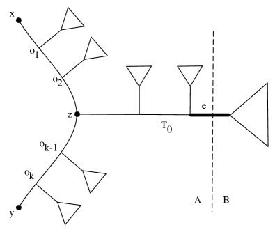
Figure 5. The collapsing lemma.

Proof: As before, we assume without loss of generality that we are using the first variant of the reduction step. Now shift the new dissimilarity map $\delta^{\prime}$ by $\frac{\delta_{T}(x,y)}{2}$ around the new taxon $z$. Again, this can be done without affecting the outcome of the algorithm. In effect, this is equivalent to defining the distances with respect to $z$ in the following manner:

$$\delta^{\prime}(z,a)=\frac{1}{2}(\delta(x,a)+\delta(y,a)-\delta_{T}(x,y)).$$

Now let $e$ be the edge in $T$ corresponding to the $A|B$ split. Let $l$ be its length. Let $p$ be the path in $T$ that joins $x$ and $y$. Then $e\not\in p$ and let $o$ be the internal point of $T$ where a path from $e$ reaches $p$. Consider the new tree $T^{\prime}$ where the taxa $x$ and $y$ are removed and the new taxon $z$ is placed exactly at the internal point $o$. $\delta_{T^{\prime}}$ and $A^{\prime}$ are defined in the obvious way and $\delta^{\prime}$ is defined by collapsing $x,y$ in $\delta$ according to the reduction described above.

Let $T_{0}\ldots T_{k}$ be the subtrees of $T$ hanging off the path $p$ and let $T_{0}$ be the one that contains $e$. We now observe that $\delta^{\prime}(a,b)=\delta(a,b)$ and $\delta_{T^{\prime}}(a,b)=\delta_{T}(a,b)$ for $a,b\neq z$. In this case the errors remain the same. For $b\in B$, and therefore $b\in T_{0}$, we observe that

$$\delta_{T^{\prime}}(z,b)=\delta_{T}(o,b)=\frac{1}{2}(\delta_{T}(x,b)+\delta_{T}(y,b)-\delta_{T}(x,y)).$$

Therefore

$$|\delta^{\prime}(z,b)-\delta_{T^{\prime}}(b,z)|=|(\delta(x,b)-\delta_{T}(x,b))+(\delta(y,b)-\delta_{T}(y,b)|\frac{1}{2}<\frac{l}{4}.$$

Now for all $i$ let $o_{i}$ be the point of the path $p$ that is the root of the subtree $T_{i}$. Then for any $a\in A$, so $a\in T_{i}$ for $i\neq 0$ or $a\in T_{0}\cap A$,

$$\delta^{\prime}(z,a)=\delta_{T^{\prime}}(a,o_{i})+[(\delta(x,a)-\delta_{T}(x,a))+(\delta(y,a)-\delta_{T}(y,a))]/2=$$

$$\delta_{T^{\prime}}(a,z)+[(\delta(x,a)-\delta_{T}(x,a))+(\delta(y,a)-\delta_{T}(y,a))]/2-\delta_{T}(o,o_{i})<$$

$$\delta_{T^{\prime}}(a,z)+\frac{l}{4}-\delta_{T}(o,o_{i}).$$

Therefore $\delta^{\prime}$ is $A^{\prime}|B$-consistent with respect to $T^{\prime}$ and $T^{\prime}$ “contains” the edge $e$.∎

Now assume that the pair $(i,j)$ which maximizes $Z_{\delta}(i,j)$ is such that $i\in A,j\in B$. Without loss of generality, we assume that $|A|\leq|B|$.

Proposition 27.

$$S(\delta:A,i,j)=\sum_{(a_{1},a_{2})\in{A\choose 2}}Z_{\delta}(a_{1},a_{2})-Z_{\delta}(i,j)>0.$$

That is, there exist $x,y\in{A\choose 2}$ such that $Z_{\delta}(x,y)>Z_{\delta}(i,j)$.

We prove the proposition by comparing the differences between the dissimilarity values and the true tree metric $\delta_{T}$, with counts of the contested edge in the averaging step. The calculation is elementary but tedious, and requires a few lemmas and some notation:

Let $M$ be the set of all dissimilarity maps $\delta:X\times X\rightarrow{\mathbb{R}}$ on a set $X$. We represent a linear function $f:M\rightarrow{\mathbb{R}}$ by

$$\delta\mapsto\sum_{\forall(a,b)\in{X\choose 2}}\alpha_{f}(a,b)\delta(a,b).$$

Similarly, if $M_{\tau}$ is the set of all tree metrics on a set $X$, we represent a linear function $f:M_{\tau}\rightarrow{\mathbb{R}}$ by

$$\delta_{T}\mapsto\sum_{\forall e\in E(T)}\beta_{f,T}(e)l(e).$$

More explicitly, $\beta_{f,T}(e)$ is the coefficient of $l(e)$ in $f(\delta_{T})$, when the metric $\delta_{T}$ corresponds to the edge lengths $l$. If $T$ is obvious from the context, we will write $\beta_{f,T}$ as $\beta_{f}$.

For a tree $T$, note that an edge $e$ divides the leaves into two sets. For a given tree leaf $i$, we define $N^{+}_{e}(i)$ as the set of leaves on the same side of $e$ as $i$ and $N^{-}_{e}(i)$ as the set of leaves on the far side of $e$ from $i$. By a slight abuse of notation, we will also use $N^{+}_{e}(i)$ and $N^{-}_{e}(i)$ to denote the number of elements in their respective sets when such use does not give rise to confusion.

Lemma 28.

Let $a,b$ be leaves in a tree $T$. Then

$$\beta_{Z(a,b)}(e)=\left\{\begin{array}[]{ll}-(N^{+}_{e}(a)-1)(N^{-}_{e}(a)-1)&\mbox{ if }e\in P_{ab};\\ &\\ N^{-}_{e}(a)(N^{-}_{e}(a)-1),&\mbox{otherwise}.\end{array}\right.$$

Proof: For a tree metric $\delta_{T}$, $w_{\delta_{T}}(ab:xy)$ is twice the length of the splitting path if $(ab:xy)$ is a quartet of $T$ and negative the length of the path otherwise. Hence, if an edge $e$ is on the path from $a$ to $b$, then there is no quartet $(ab:xy)$ such that $e$ is on the splitting path. Hence, the edge $e$ is only counted negatively, once for every element $x\in N^{+}_{e}(a)-\{a\}$ and $y\in N^{+}_{e}(b)-\{b\}=N^{-}_{e}(a)-\{b\}$. There are exactly $(N^{+}_{e}(a)-1)(N^{-}_{e}(a)-1)$ such pairs $(x,y)$.

If $e$ is not on the path from $a$ to $b$, then for any pair of elements $(x,y)\in{N^{-}_{e}(a)\choose 2}$, $(ab:xy)$ are exactly the quartets of $T$ of the form $(ab:\cdot\cdot)$ with $e$ is on the splitting path. Consequently, $\beta_{Z(a,b)}(e)=2{N^{-}_{e}(a)\choose 2}=N^{-}_{e}(a)(N^{-}_{e}(a)-1)$. ∎

Lemma 29.

Let an edge $e$ define a split $A|B$ and assume $|A|\leq|B|$. Then

$$S(\delta_{T}:A,i,j)\geq{|A|\choose 2}(|B|-1)(n-1)l(e).$$

Proof: This is equivalent to showing that

$$\beta_{S(\delta_{T}:A,i,j)}(e)={|A|\choose 2}(|B|-1)(n-1),$$

and for any other edge $e^{\prime}\in T$, $\beta_{S(\delta_{T})}(e^{\prime})\geq 0$. Note that since $e$ is never on the path between $a_{1}$ and $a_{2}$ for any pair $a_{1},a_{2}\in A$, $\beta_{Z(a_{1},a_{2})}$ is the same for any choice of $a_{1},a_{2}$. Also, $e$ is on the path between $i$ and $j$, so by application of Lemma 28:

$$\beta_{S(\delta_{T}:A,i,j)}(e) = \sum_{(a_{1},a_{2})\in{A\choose 2}}\beta_{Z(a_{1},a_{2})}(e)-\beta_{Z(i,j)}(e)$$

$$= {|A|\choose 2}[\beta_{Z(a_{1},a_{2})}(e)-\beta_{Z(i,j)}(e)]$$

$$= {|A|\choose 2}[|B|(|B|-1)+(|A|-1)(|B|-1)]$$

$$= {|A|\choose 2}(|B|-1)(n-1).$$

Let $t$ be either vertex of the edge $e$. Assume we have an edge $e^{\prime}\neq e$ such that $e^{\prime}$ is in the subtree spanned by $B$, denoted $e^{\prime}\in[B]$. Then $e^{\prime}$ is never on the path between $a_{1}$ and $a_{2}$, so $\beta_{Z(a_{1},a_{2})}(e^{\prime})=N^{-}_{e^{\prime}}(t)(N^{-}_{e^{\prime}}(t)-1)$ for any pair $a_{1},a_{2}\in A$. If $e^{\prime}$ is on the path between $i$ and $j$, then $\beta_{Z(i,j)}(e^{\prime})<0$, so clearly $\beta_{S(\delta_{T}:A,i,j)}(e^{\prime})>0$. If $e^{\prime}$ is not on the path between $i$ and $j$, then $\beta_{Z(i,j)}(e^{\prime})=\beta_{Z(a_{1},a_{2})}(e^{\prime})$ and $\beta_{S(\delta_{T})}(e^{\prime})=0$. The proof of the final case that needs to be considered, namely $e^{\prime}\in[A]$ consists of a trivial, yet slightly lengthy, counting argument. We only present a brief sketch.

Again, in the case when $e^{\prime}$ is on the path between $i$ and $j$, then $\beta_{Z(i,j)}(e^{\prime})<0$, so clearly $\beta_{S(\delta_{T}:A,i,j)}(e^{\prime})>0$. For $e^{\prime}$ not on the path from $i$ to $j$, let $A^{\prime}=N_{e^{\prime}}^{-}(i)\subset A$. Let $\alpha=|A^{\prime}|$. Then a simple counting argument shows that $\beta_{Z(i,j)}(e^{\prime})=2{\alpha\choose 2}$, whereas for $f=\sum_{(a_{1},a_{2})\in{A\choose 2}}Z_{\delta}(a_{1},a_{2})$ we have $\beta_{f}(e^{\prime})=2{\alpha\choose 2}{|B|\choose 2}$. Since $|B|>|A|$, this concludes the proof. ∎

Lemma 30.

Let $a,b$ be elements of the leaf set $X$ of size $n$. Then:

$$\alpha_{Z(a,b)}(x,y)=\left\{\begin{array}[]{ll}-{n-2\choose 2}&\mbox{ if }|\{a,b\}\cap\{x,y\}|=2;\\ &\\ \frac{1}{2}(n-3)&\mbox{ if }|\{a,b\}\cap\{x,y\}|=1;\\ &\\ -1&\mbox{ if }|\{a,b\}\cap\{x,y\}|=0.\end{array}\right.$$

Proof: The term $\delta(a,b)$ occurs in all ${n-2\choose 2}$ $w(ab:xy)$ terms in $Z(a,b)$, each time with a coefficient of $-1$. To compute $\alpha_{Z(a,b)}(a,x)$, we note that $\delta(a,x)$ occurs in all $(n-3)$ terms of the form $w(ab:x\cdot)$ with a coefficient of $\frac{1}{2}$. The same holds for $\alpha_{Z(a,b)}(b,x)$. Lastly, $\delta(x,y)$ for $x,y\neq a,b$ occurs only in one term, $w(ab:xy)$, with coefficient $-1$. ∎

Lemma 31.

Let $a,a_{1}\neq a_{2}\in A-\{i\}$ and $b,b_{1}\neq b_{2}\in B-\{j\}$. We have

1. $\alpha_{S(\delta)}(i,j)=\frac{1}{2}(|A|-1)(|B|-1)+{|A|\choose 2}{n-2\choose 2},$
   

2. $\alpha_{S(\delta)}(i,a)=-{|B|\choose 2}-\frac{1}{2}(n-3){|A|\choose 2},$
   

3. $\alpha_{S(\delta)}(j,a)=\frac{1}{2}(|A|-1)(|B|-1)-\frac{1}{2}(n-3){|A|\choose 2}=-\frac{1}{4}(n-1)(|A|-1)(|A|-2),$
   

4. $\alpha_{S(\delta)}(i,b)=\frac{1}{2}(|A|-1)(|B|-1)-\frac{1}{2}(n-3){|A|\choose 2}=-\frac{1}{4}(n-1)(|A|-1)(|A|-2),$
   

5. $\alpha_{S(\delta)}(j,b)=-{|A|\choose 2}-\frac{1}{2}(n-3){|A|\choose 2},$
   

6. $\alpha_{S(\delta)}(a,b)=\frac{1}{2}(|A|-1)(|B|-1)+{|A|\choose 2},$
   

7. $\alpha_{S(\delta)}(a_{1},a_{2})=-{|B|\choose 2}+{|A|\choose 2},$
   

8. $\alpha_{S(\delta)}(a_{1},a_{2})=-{|A|\choose 2}+{|A|\choose 2}=0.$
   

There are $1,|A|-1,|A|-1,|B|-1,|B|-1,(|A|-1)(|B|-1),{|A|-1\choose 2}$ and ${|B|-1\choose 2}$ of each of these terms, respectively.

Proof: Let $S_{1}(\delta)=\sum_{(a_{1},a_{2})\in{A\choose 2}}Z_{\delta}(a_{1},a_{2})$ Note that

$$\alpha_{S_{1}(\delta)}(x,y)=\left\{\begin{array}[]{ll}-{|B|\choose 2}&\mbox{ if }|\{x,y\}\cap A|=2;\\ &\\ \frac{1}{2}(|A|-1)(|B|-1)&\mbox{ if }|\{x,y\}\cap A|=1;\\ &\\ -{|A|\choose 2}&\mbox{ if }|\{x,y\}\cap A|=0.\end{array}\right.$$

We provide the proof for the first case, where $x,y\in A$ (the other cases are similar). Let $A^{\prime}=A-\{x,y\}$, then:

$$\alpha_{S_{1}(\delta)} = \alpha_{Z_{\delta}(x,y)}(x,y)+\sum_{a\in A^{\prime}}\alpha_{Z_{\delta}(a,x)}(x,y)+\alpha_{Z_{\delta}(a,y)}(x,y)+\sum_{a_{1},a_{2}\in{A^{\prime}\choose 2}}\alpha_{Z_{\delta}(a_{1},a_{2})}(x,y)$$

$$= -{n-2\choose 2}+|A^{\prime}|\left[\frac{1}{2}(n-3)+\frac{1}{2}(n-3)\right]+{|A^{\prime}|\choose 2}(-1)$$

$$= \frac{1}{2}(n-|A|)\left[|A|-n+1\right]\quad=\quad-{|B|\choose 2}.$$

Identities (1)–(8) now follow after some elementary algebra and Lemma 30.∎

Lemma 32.

$$S(\delta_{T})-S(\delta)<\frac{l}{8}(|A|-1)(n-1)(3|A|n-2n-2|A|^{2}-4|A|+4)$$

Proof: Let $\delta$ be an $A|B$-consistent metric and set $\tilde{\delta}=\delta_{T}-\delta$. Note that for all $x,y\in{X\choose 2}$,

$$\alpha_{S(\tilde{\delta})}(x,y)\tilde{\delta}(x,y)<|\alpha_{S(\tilde{\delta})}(x,y)|\frac{l}{4}.$$

This follows directly from the fact that $\alpha_{S(\delta)}(x,y)<0$ for all cases where $x,y\in A$ or $x,y\in B$, together with the signs of the terms in the Lemma 31 and the definition of $A|B$-consistency. It follows that

$$S(\tilde{\delta})=\sum_{x,y\in{X\choose 2}}\alpha_{S(\tilde{\delta})}(x,y)\tilde{\delta}(x,y)<\sum_{x,y\in{X\choose 2}}|\alpha_{S(\tilde{\delta})}(x,y)|\frac{l}{4},$$

and the lemma follows by summing the terms appearing in Lemma 31.∎

Proof of Proposition 27 and Theorem 25: By Lemma 29 and 32 it suffices to show that

$$\frac{l}{2}|A|(|A|-1)(|B|-1)(n-1)-\frac{l}{8}(|A|-1)(n-1)(3|A|n-2n-2|A|^{2}-4|A|+4)\geq 0.$$

This inequality follows from the fact that we chose $|A|\leq|B|$ and consequently $2|A|\leq n$. Thus, the pair of leaves that maximize $(Z\cdot,\cdot)$ are both in $A$. The theorem now follows from Proposition 26. ∎

We conclude by stating that our analysis holds trivially for the fast neighbor-joining algorithm of [6]. This follows from the observation that for an $A|B$-consistent dissimilarity map $\delta$, no pair $x,y$ with $x\in A$ and $y\in B$ can maximize the $Z(\cdot,\cdot)$ criterion, and therefore the maximizing pair, which has to be visible from both of its members, has both taxa on the same side of the partition $A|B$.

Corollary 33.

If $\delta$ is an $A|B$-consistent dissimilarity map with respect to a tree $T$, then FNJ applied to $\delta$ will reconstruct a tree $T^{\prime}$ which contains $A|B$ among its set of edge-induced splits.

We conclude with a final comment on $A|B$-consistency and our proof of Theorem 25.

Theorem 34.

Let $\delta_{T}$ be a tree metric and $\delta$ a dissimilarity map whose $l_{\infty}$ distance to $\delta_{T}$ is less than $\frac{\beta}{4}$ where $\beta$ is the length of some edge in $T$. Then it may be that an intermediate tree produced during the agglomeration steps of the neighbor-joining algorithm has $l_{\infty}$ distance greater than $\frac{\beta}{4}$ to any tree metric.

Proof: Consider the phylogenetic tree $T$ in Figure 6, with leaf set $S=X\cup\{i,j,a,b\}$ where $|X|=n$. Suppose that the leaf edges corresponding to $i,j,a,b$ all have length $\alpha$. The lengths of the other visible edges, i.e. the ones not belonging to $T|_{X}$ are as in Figure 6. Also suppose that the edges on the subtree $T|_{X}$ have total length $\leq\epsilon$, where we will let $\epsilon$ become arbitrarily small.

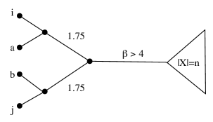
Figure 6. Example for Theorem 34.

Consider the following dissimilarity map $\delta$ with $||\delta-\delta_{T}||_{\infty}=1$:

1. $\delta(i,j)=\delta_{T}(i,j)-1,$

2. $\delta(p)=\delta_{T}(p)+1$ for $p=(a,b),(a,i),(b,j),$

3. $\delta(p)=\delta_{T}(p)$ for $p=(a,j),(b,i),$

4. $\delta(x,y)=\delta_{T}(x,y)$ for $x,y\in X,$

5. $\delta(i,x)=\delta_{T}(i,x)+1$ for $x\in X,$

6. $\delta(j,x)=\delta_{T}(j,x)+1$ for $x\in X,$

7. $\delta(a,x)=\delta_{T}(a,x)-1$ for $x\in X,$

8. $\delta(b,x)=\delta_{T}(b,x)-1$ for $x\in X.$

Minimizing the neighbor-joining $Q$ criterion is equivalent to maximizing

$$Y_{\delta}(k,l)=2\delta(k,l)+\sum_{t\in S-\{k,l\}}\delta_{k,l}(t)$$

where $\delta_{k,l}(t)=\delta(k,t)+\delta(l,t)-\delta(k,l)$.

First we show that for large enough $n$, small enough $\epsilon$ and with $\beta>4$, the pair that maximizes $Y$ is $(i,j)$. Note that for $x,y\in X$, $Y(x,y)=\sum_{t\in\{i,j,k,l\}}2\delta_{x,y}(t)+O(\epsilon)$, which converges to a constant as $\epsilon\rightarrow 0$. However, as $n\rightarrow\infty$, $Y(i,j)\approx 2n\beta$. Therefore for small enough $\epsilon$ and large enough $n$, $(i,j)$ will dominate any pair $(x,y)\in{X\choose 2}$. Since $\beta>4$ and $||\delta-\delta_{T}||_{\infty}=1$, using a similar argument as above we can also conclude that the optimum pair must consist of two leaves from $\{i,j,a,b\}$.

Finally, we need to show that $Y(i,j)>Y(k,l)$ where either $k$ or $l$ is equal to $a$ or $b$. Note that for any $k,l\in\{i,j,a,b\}$,

$$Y(k,l)=2\delta(k,l)+\sum_{t\in\{a,b\}\}}\delta_{k,l}(t)+\sum_{t\in X}\delta_{k,l}(t).$$

The first and second summands are constants in $n$, while the third is composed of $n$ sub-terms which are roughly equal, up to small variations of size at most $O(\epsilon)$, depending on the location of $t$ in $T|_{X}$. Since we can choose $\epsilon$ arbitrarily small, we can therefore ignore this error. Now place a fictitious node $v$ at the root of $T|_{X}$ (the right hand side of the edge of length $\beta$).Then letting $n\rightarrow\infty$, we see that asymptotically,

$$Y(k,l)\approx n\delta_{k,l}(v).$$

Here we extend the definition of $\delta$ to $v$ by extending $\delta_{T}$ to $v$ in the natural way and defining the error $\delta-\delta_{T}$ for pairs involving $v$ in the same way as for other leaves in $X$. It is now easy to verify that

1. $\delta_{i,j}(v)=\delta(i,v)+\delta(j,v)-\delta(i,j)=2(\alpha+\beta+1.75)+1+1-(2\alpha+3.5-1)=2\beta+3$,

2. $\delta_{i,a}(v)=\delta_{j,b}(v)=\delta(i,v)+\delta(a,v)-\delta(i,a)=2(\alpha+\beta+1.75)+1-1-(2\alpha+1)=2\beta+2.5$,

3. $\delta_{j,a}(v)=\delta_{i,b}(v)=\delta(j,v)+\delta(a,v)-\delta(j,a)=2(\alpha+\beta+1.75)+1-1-(2\alpha+3.5)=2\beta$,

4. $\delta_{a,b}(v)=\delta(a,v)+\delta(b,v)-\delta(a,b)=2(\alpha+\beta+1.75)-1-1-(2\alpha+3.5+1)=2\beta-3$.

Therefore asymptotically, $(i,j)$ will be collapsed in the first step of neighbor-joining applied to $\delta$.

Now consider the reduced distance matrix $\delta^{\prime}:S^{\prime}\times S^{\prime}\rightarrow\mathbb{R}$, where the leaves $i$ and $j$ are replaced by a new leaf $u$. That is, $S^{\prime}=S-\{i,j\}\cup\{u\}$. We restrict our attention to the set $\{a,b,u,x\}$ for an arbitrary leaf of $x$ of $X$. Since the total length of $T|_{X}$ is $O(\epsilon)$, we can in fact approximate expressions involving $\delta(\dot{,}x)$ by $\delta(\dot{,}v)$ up to $O(\epsilon)$ error. We do so for the sake of simplicity.

Simple calculations now give

$$\delta^{\prime}(a,u)=\delta^{\prime}(b,u)=2\alpha+2.25,$$

$$\delta^{\prime}(a,x)=\delta^{\prime}(b,x)=\alpha+\beta+.75,$$

$$\delta^{\prime}(a,b)=\delta(a,b)=2\alpha+3.5,$$

$$\delta^{\prime}(u,x)=\alpha+\beta+2.75,$$

and thus:

$$\delta^{\prime}(a,u)+\delta^{\prime}(x,b)=\delta^{\prime}(b,u)+\delta^{\prime}(x,a)=\delta^{\prime}(x,u)+\delta^{\prime}(a,b)-4.25=\beta+3\alpha+3.$$

Now suppose that there is some additive tree metric $\mu$ such that $||\delta^{\prime}-\mu||_{\infty}\leq 1$. Then by adding this to the above equality we obtain that

$$\mu(x,u)+\mu(a,b)-\mu(b,u)-\mu(x,a)\geq 4.25-4>0$$

and similarly

$$\mu(x,u)+\mu(a,b)-\mu(a,u)-\mu(x,b)\geq 4.25-4>0.$$

This contradicts the four point condition necessary for $\mu$ to be a tree metric. Therefore, we have given an example of a dissimilarity map $\delta$ and a tree metric $\delta_{T}$ with an edge of length $\beta$, such that $||\delta-\delta_{T}||_{\infty}<\frac{\beta}{4}$, and yet the $l_{\infty}$ distance of the reduced dissimilarity map after the first agglomeration step from any tree metric is greater than $\frac{\beta}{4}$. ∎

The significance of Theorem 34 is that it shows that an inductive proof of Atteson’s conjecture is not possible without relaxing the hypothesis. Thus, the partial result of [30] and the proof of [4] are incorrect. At the same time, Theorem 34 also identifies an undesirable property of neighbor-joining which is very common among greedy optimization algorithms. We hope that further investigations in this direction can yield more robust versions of the algorithm.

6. Simulation results and conclusion

We performed a series of simulations to test how frequently Theorem 16 explains the success of the neighbor-joining algorithm. Trees with 20 taxa were generated by agglomerating pairs at random. We generated 35 such trees and set their edge lengths to 0.1. We then used seq-gen [22] to build 100 alignments with the Jukes Cantor model for each of 28 sequence lengths between 100 and 10,000 base pairs. From these we obtained dissimilarity maps using the dnadist program from the PHYLIP package [9]. Our Java API then computed the $w$-matrix for each dissimilarity map, tested the consistency and additivity conditions against the true tree, checked to see if the dissimilarity map satisfied Atteson’s criterion (Theorem 2), and computed the neighbor-joining tree. The results are summarized in Figure 7.

We note that our conditions of additivity and consistency are satisfied for sequence lengths an order of magnitude smaller than required for Atteson’s criterion to hold. Moreover, even when the additivity and consistency conditions are not satisfied for every quartet, they do hold true for upwards of 99% and 94% of quartets respectively, even at sequence length 100 (Figure 7). Hence, applying an averaging argument similar to the one we employed in the proof of Atteson edge radius conjecture, we may obtain “on average” conditions that explain even more of the cases where neighbor-joining succeeds.

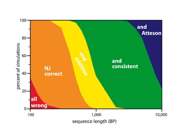
Figure 7. Conditions satisfied as a function of sequence length. 35 trees with 20 taxa each were simulated 100 times for 28 different sequence lengths. 100 alignments were generated for each tree. The figure shows, for each of the 9800000 dissimilarity maps generated from the simulations, whether neighbor-joining reconstructed the correct tree, and whether additivity, consistency and Atteson’s criterion were satisfied. Note that the x-axis is logarithmic.

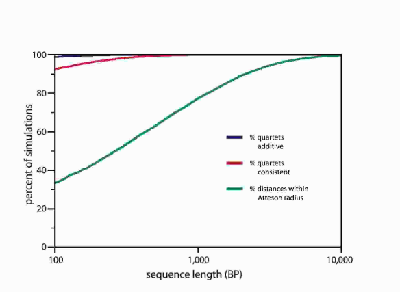
Figure 8. Details on the percent of quartets satisfying the additivity and consistency conditions when neighbor-joining succeeds. The green curve shows the number of distances within the Atteson radius.

7. Acknowledgments

Radu Mihaescu was supported by a National Science Foundation graduate fellowship, and partially by the Fannie and John Hertz Foundation. Lior Pachter was partially supported by NIH grant R01HG2362 and NSF grant CCF0347992. Dan Levy was supported by NIH grant GM68423.

References

- [1] K Atteson, The performance of neighbor-joining methods of phylogenetic reconstruction, Algorithmica 25 (1999), 251–278.
- [2] WJ Bruno, ND Socci, and AL Halpern, Weighted neighbor-joining: a likelihood-based approach to distance-based phylogeny reconstruction, Molecular Biology and Evolution 17 (2000), no. 1, 189–197.
- [3] D Bryant, On the uniqueness of the selection criterion in neighbor-joining, Journal of Classification 22 (2005), no. 1, 3–15.
- [4] W Dai and Y Xu and B Zhu, On the edge radius of Saitou and Nei’s method for phylogenetic reconstruction, Theoretical Computer Science 369 (2006), no. 1–3, 448–455.
- [5] R Desper and O Gascuel, The minimum evolution distance-based approach to phylogenetic inference, Mathematics of Evolution and Phylogeny (O Gascuel, ed.), Oxford University Press, 2005.
- [6] I Elias and J Lagergren, Fast neighbor joining, Proceedings of the International Colloquium on Automata, Languages and Programming (ICALP ’05), 2005.
- [7] PL Erdös, MA Steel, LA Székely, and TJ Warnow, A few logs suffice to build (almost) all trees. I, Random Structures and Algorithms 14 (1999), no. 2, 153–184.
- [8] JS Farris, VA Albert, M Källersjö, D Lipscomb, and AG Kluge, Parsimony jackknifing outperforms neighbor-joining, Cladistics 12 (1996), 99–124.
- [9] J Felsenstein, PHYLIP (phylogeny inference package) version 3.5c., Tech. report, Department of Genetics, University of Washington, Seattle, 1993.
- [10] O Gascuel, A note on Sattath and Tversky’s, Saitou and Nei’s, and Studier and Keppler’s Algorithms for Inferring Phylogenies from Evolutionary Distances, Molecular Biology and Evolution 11 (1994), no. 6, 961–963.
- [11] by same author, BIONJ: an improved version of the NJ algorithm based on a simple model of sequence data, Molecular Biology and Evolution 14 (1997), no. 7, 685–695.
- [12] O Gascuel and M Steel, Neighbor-joining revealed, Molecular Biology and Evolution 23 (2006), no. 11, 1997–2000.
- [13] BG Hall, Comparison of the accuracies of several phylogenetic methods using protein and DNA sequences, Molecular Biology and Evolution 22 (2005), no. 3, 792–802.
- [14] J Huelsenbeck and D Hillis, Success of phylogenetic methods in the four-taxon case, Systematic Biology 42 (1993), no. 3, 247–264.
- [15] K St. John, T Warnow, B Moret, and L Vawter, Performance study of phylogenetic methods: (unweighted) quartet methods and neighbor joining, Journal of Algorithms 48 (2003), 174–193.
- [16] MK Kuhner and J Felsenstein, A simulation comparison of phylogeny algorithms under equal and unequal evolutionary rates, Molecular Biology and Evolution 11 (1994), 459–468.
- [17] S Kumar and SR Gadagker, Efficiency of the neighbor-joining method in reconstructing evolutionary relationships in large phylogenies, Journal of Molecular Evolution 51 (2000), 544–553.
- [18] D Levy, R Yoshida, and L Pachter, Beyond pairwise distances: neighbor joining with phylogenetic diversity estimates, Molecular Biology and Evolution 23 (2006), 491–498.
- [19] GJ Olsen, H Matsuda, R Hagstrom, and R Overbeek, fastDNAml: A tool for construction of phylogenetic trees of DNA sequences using maximum likelihood, Computational Applied Biosciences 10 (1994), 41–48.
- [20] S Ota and WH Li, NJML: A hybrid algorithm for the neighbor-joining and maximum likelihood methods, Molecular Biology and Evolution 17 (2000), no. 9, 1401–1409.
- [21] Y Pauplin, Direct calculation of tree length using a distance matrix, Journal of Molecular Evolution 51 (2000), 41–47.
- [22] A Rambaut and N C Grassly, Seq-Gen: an application for the Monte Carlo simulation of DNA sequences evolution along phylogenetic trees, Computational Applied Bioscience 13 (1997), 235–238.
- [23] V Ranwez and O Gascuel, Improvement of distance-based phylogenetic methods by a local maximum likelihood approach using triplets, Molecular Biology and Evolution 19 (2002), no. 11, 1952–1963.
- [24] N Saitou and M Nei, The neighbor joining method: a new method for reconstructing phylogenetic trees, Molecular Biology and Evolution 4 (1987), no. 4, 406–425.
- [25] S Sattath and A Tversky, Additive similarity trees, Psychometrika 42 (1977), no. 6, 319–345.
- [26] C Semple and M Steel, Phylogenetics, Oxford University Press graduate series in Mathematics and its Applications (2003).
- [27] K Strimmer and A von Haeseler, Quartet puzzling: A quartet maximum likelihood method for reconstructing tree topologies, Molecular Biology and Evolution 13 (1996), 964–969.
- [28] JA Studier and KJ Keppler, A note on the neighbor-joining method of Saitou and Nei, Molecular Biology and Evolution 5 (1988), 729–731.
- [29] K Tamura, M Nei, and S Kumar, Prospects for inferring very large phylogenies by using the neighbor-joining method, Proceedings of the National Academy of Sciences 101 (2004), 11030–11035.
- [30] Y Xu, W Dai, and B Zhu, A lower bound on the edge radius of Saitou and Nei’s method for phylogenetic reconstruction, Information Processing Letters 94 (2005), 225–230.