Quasi-Linear Soft Tissue Models Revisited

Abstract

Incompressibility, nonlinear deformation under stress and viscoelasticity are the fingerprint of soft tissue mechanical behavior. In order to model soft tissues appropriately, we must pursue to complete these requirements. In this work we revisited different soft tissue quasi-linear model possibilities in trying to achieve for this commitment.

I Introduction

Different mechanical properties of biological tissues depend on mineral content. Thus, roughly, it can be distinguished two classes of biological tissues. Bones and tooth content mineral, they conform the group known as hard tissues. Whereas, skin, muscle, blood vessel and lungs conform the second group called of soft tissues. They do not content mineral, so they are much deformable than hard tissues.

Modelling the mechanical behavior of soft tissues has much in common with those techniques used to model rubber elasticity. Thus, finite deformation theories useful for rubber elasticity are often used to describe soft tissue mechanical behavior. However, there are significant differences in the material structure of soft tissues and rubber elasticity. Moreover, in the way they respond under applied stress. Soft tissue material achieve initially large stretch under relatively low level of stress and subsequent stiffening at higher level extensions. This is shown in Figure( 1), where are compared the typical simple tension stress-stretch response of rubber (left-hand figure) with that of soft tissue (right-hand figure). For other side, collagen fibres distribution leads to pronounced anisotropy in soft tissue, in contrast with from typical isotropic rubber ogden ; holzapfel ; holzapfel2 .

In biomechanics an specimen (animal) is regarded as an assemble of rigid bodies connected by joins and muscles. Under this framework, Newton’s law balance of forces maybe could not be efficient to write equations of motion for each connectors, known their mechanical properties. Naturally, because the number of particles to be considered is excessively large, and the way to specify the interaction forces between particles becomes very complex. Instead, it is much better to consider the body as a continuum, searching for a simplified way to specify interaction forces between particles by means of constitutive equations, and so thus specifying realistic properties of materials. A stress-strain relationship describes the mechanical property of a material and it is therefore a constitutive equation.

Research on modelling soft tissue mechanical behavior has a growing demand for applications in surgical simulations, pursuing for in real time fast and precise calculations of tissue deformations. In trying for these commitments, it has been introduced models accounting for the continuous nature of soft tissue. Within the limits of the employed constitutive model the finite element methods allows for physically correct simulation of the tissue mechanics bro-nielsen ; keeve ; koch . For other side, alternative discrete approaches based on spring-mass model have also been appliedmosegaard ; tescher . It seems that methods based on the continuum approach are more appropriated to describe much better realistic soft tissue mechanical behavior, whereas spring-mass based models being economics are less accurate than the former. The main issue of our research look for an appropriate way to establish an accurate comparison between these methodologies.

In this work we review some physic models applicable to modelling soft tissue mechanical behavior and we also discuss some perspective in the field. This work is organized as follow: In section II we present the continuum approach formalism, and we also consider particular mathematical results for linear elastic solids and fluids. Important testing methods on physics necessaries to characterize soft tissue mechanical behavior, i.e, strain, creep and relaxation, are presented in section III. Next, in section IV are reviewed more general soft tissue mechanical properties. Section V is devoted to show basic mathematic models describing nonlinear elasticity and quasi-linear viscoelasticity, which are related to soft tissue mechanical behavior. In section VI, it is presented the basic vibrational spring-mass model, which is also extended to consider viscoelastic mechanical behavior. In section VII we presented some discussions and perspectives.

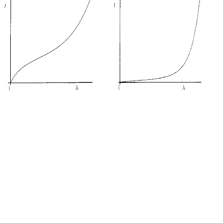
Figure 1: Typical simple tension response of (a) rubber and (b) soft tissue. Nominal stress $t>0$ plotted against stretch $\lambda\geq\,1$ .

II Continuum Approach

The equations of motion for a continuum were derived by Euler, using Newton’s laws and supported on the follow axioms: i) The material particles form a one-to-one isomorphism with real numbers in a $3\mathcal{D}$ Euclidean space. ii) The mass distribution is characterized by the density $\rho$ (the mass per unit volume), it is defined as a piecewise continuous function over the volume of the continuum. iii) Solely neighbors particle interactions are regarded. A surface is conformed by particles, it could be considered arbitrarily infinitesimal. In a continuum, oriented surfaces interaction can be expressed as a surface traction ( Force per unit area), that can be computed from a well defined stress tensor ($\sigma_{ij}\,$).

Let us $x_{1},x_{2},x_{3}$ be an inertial cartesian frame of reference, and an infinitesimal volume by $dx_{1}dx_{2}dx_{3}$. Let $\sigma_{ij},\,e_{ij}$ be the stress and strain tensor, respectively. Let us denote: $v_{i},\,D\,v_{i}/Dt$ and $X_{i}$; the velocity vector, the acceleration vector and the body force per unit volume, respectively. We now recall Newton’s balance of forces, stating that the material rate of change of the linear momentum of a body must be equal to the resultant of forces applied to the body. In follow, we write it in the form of Euler’s equation, for more details see fung :

$$v_{i}\left(\frac{\partial{\rho}}{\partial{t}}+\frac{\partial{\rho}v_{j}}{\partial{x}_{j}}\right)+\rho\frac{Dv_{i}}{Dt}=\frac{\partial\sigma_{ij}}{\partial{x}_{j}}+X_{i}\,.$$ (1)

Using tensor notation, a repetition of an index in any given term means a summation over the range of that index,

$$\frac{\partial\sigma_{ij}}{\partial{x}_{j}}=\frac{\partial\sigma_{i1}}{\partial{x}_{1}}+\frac{\partial\sigma_{i2}}{\partial{x}_{2}}+\frac{\partial\sigma_{i3}}{\partial{x}_{3}}\,.$$

In the spatial description,

$$\frac{Dv_{i}}{Dt}=\frac{\partial\,v_{i}}{\partial\,t}+v_{j}\frac{\partial\,v_{i}}{\partial\,x_{j}}\,.$$

By taking into account the conservation of mass, expressed by the equation of continuity:

$$\frac{\partial\rho}{\partial{t}}+\frac{\partial\rho\,v_{j}}{\partial{x_{j}}}\equiv\,\frac{D\rho}{Dt}+\rho\frac{\partial{v_{j}}}{\partial{x_{j}}}\,=0\,,$$ (2)

Eqn.( 1) becomes,

$$\rho\frac{Dv_{i}}{Dt}=\frac{\partial\sigma_{ij}}{\partial\,x_{j}}+X_{i}\,\hskip 28.45274pt\,\left(i=1,2,3\right)\,.$$ (3)

This is valid for any continuum, whether it is a fluid or a solid.

In particular, if the material is considered to be incompressible, regarded $\rho$ is a constant; we get from the Eqn.( 2),

$$\partial\,v_{j}/\partial\,x_{j}=0\,.$$ (4)

From here, further development requires specification of the properties of the material in the form of constitutive equations, relating stress with strain or strain rate; or strain history. In order to have a complete theory, all these constitutive relationship must be incorporated into Eqn.( 3).

Using our faculty perceptions we can verify: booth skin and muscle have a definite shape, they even can sustain a shear force, and maintains a quasi-static state (i.e. stress is a function of strain). Therefore, their mechanical behavior is analogous to that one of a solid. Whereas considering blood (at least in normal conditions) we note: it has no shape, it can not sustain a shear force (because it is in motion), and given its dynamic state; the stress is a function of the rate of strain. Thus it behaves mechanically like a fluid.

Next, we derive particular equations for isotropic solid materials which follow Hook’s elastic law and also for Newtonian fluids using Euler’s formalism, incorporating specific constitutive relationships.

II.1 Isotropic Hookean Solid

These kind of materials obey the following stress-strain linear relationship:

$$\sigma_{ij}=\lambda\,e_{kk}\delta_{ij}+2\,G\,e_{ij}\,;$$ (5)

which alternative inverse relationship can be re-written as,

$$e_{ij}=\frac{1+\nu}{E}\sigma_{ij}-\frac{\nu}{E}\sigma_{kk}\delta_{ij}\,,$$

where $\sigma_{ij}$ and $e_{ij}$ are the stress and strain tensors, $\lambda$ is the Lamé constant, $G$ is the shear modulus, $E$ is the Young’s modulus and $\nu$ is the Poisson’s ratio. $\delta_{ij}$ is the Kronecker delta (unity if $i=j$, otherwise is zero ). We see here that, the strain is being referred to a configuration of the body in which it is null provided that the stress is zero.

Substituting Eqn.( 5) into Eqn.( 3) we arrived to,

$$\rho\frac{Dv_{i}}{Dt}=\lambda\frac{\partial{e}_{\alpha\alpha}}{\partial{x}_{i}}+2G\frac{\partial{e}_{ij}}{\partial{x}_{j}}+X_{i}\,.$$ (6)

Lets now denote the vector displacement of a point in the body by $\mathit{u}_{i}$, which is measured with respect to an inertial cartesian frame of reference. If $\mathit{u}_{i}(x_{1},x_{2},x_{3},t)$ is infinitesimal, we can define,

$$e_{ij}=\frac{1}{2}\left(\frac{\partial\mathit{u}_{i}}{\partial\,x_{j}}+\frac{\partial\mathit{u}_{j}}{\partial\,x_{i}}\right)\,.$$ (7)

To the same order of approximation,

$$v_{i}=\frac{\partial\mathit{u}_{i}}{\partial\,t}\,,\hskip 28.45274pt\,\frac{Dv_{i}}{Dt}=\frac{\partial^{2}\mathit{u}_{i}}{\partial\,t^{2}}\,.$$ (8)

On substituting all these equations into Eqn.( 6), it is obtained the well known Navier’s equation:

$$\rho\frac{\partial^{2}\mathit{u}_{i}}{\partial{t}^{2}}\,=\,G\frac{\partial^{2}\mathit{u}_{i}}{\partial{x}_{j}\partial{x}_{j}}+\frac{G}{1-2\nu}\frac{\partial}{\partial{x}_{i}}\frac{\partial\mathit{u}_{j}}{\partial{x}_{j}}+X_{i}\,,$$ (9)

where the Poissons’ ratio $\nu=\frac{\lambda}{2\left(\lambda\,+\,G\right)}$. In this way, we arrived to the basic field equation of the linearized theory of elasticity. However, living bodies often take on finite deformations, obey so more complex nonlinear constitutive equations than the above presented.

II.2 Newtonian Fluid

These fluids obey the following stress-strain-rate relationship,

$$\sigma_{ij}=-\mathit{p}\,\delta_{ij}\,+\,\mu\left(\frac{\partial{u}_{i}}{\partial{x}_{j}}+\frac{\partial{u}_{j}}{\partial{x}_{i}}\right)\,+\,\lambda\left(\frac{\partial{u}_{k}}{\partial{x}_{k}}\right)\,\delta_{ij}\,,$$ (10)

where $\mathit{p}$ is the pressure, $\mu$ is the dynamic viscosity ( a constant parameter), and $\lambda$ is the bulk elasticity ( second coefficient of viscosity). If the fluid is incompressible, according to Eqn.( 4), this expression simplified to,

$$\sigma_{ij}=-\mathit{p}\,\delta_{ij}+\mu\,\left(\frac{\partial{u}_{i}}{\partial{x}_{j}}+\frac{\partial{u}_{j}}{\partial{x}_{i}}\right)\,.$$ (11)

By substituting it into Eqn.( 2), we obtain the Navier-Stokes equation, valid for Newtonian fluids,

$$\frac{\partial\mathit{u}_{i}}{\partial{t}}+\mathit{u}_{j}\frac{\partial\mathit{u}_{i}}{\partial{x}_{j}}=-\frac{1}{\rho}\frac{\partial\mathit{p}}{\partial{x}_{i}}\,+\,\nu\frac{\partial^{2}\mathit{u}_{i}}{\partial{x}_{j}\partial{x}_{j}}\,+\,X_{i}\,,$$ (12)

where $\nu\,\left(=\mu/\rho\right)$ is the fluid kinematic viscosity. Appropriate boundary conditions are necessary in order to solve the current equation.

Air and water are Newtonian fluids. Non-Newtonian fluids do not obey constitutive equations ( 12). Like blood, most body fluids are non-Newtonian. However at a shear strain rate above $100\,sec^{-1}$ blood is almost Newtonian.

In general, soft tissues present unique mechanical properties. In the next section we present some basic test methods useful to describe quantitative soft tissue mechanical properties.

III Test Methods

The tensile test method consists to measure deformation of an specimen while a force being applied to a sample is gradually increased. During the stretching process are measured both, the stress and the strain. The former is obtained taking the ratio of the force and the material cross sectional area, whereas the latter is derived dividing the displacement and the original material length. Analyzing the stress-strain curve provides useful information: as said the Young’s module, the yield point and the ultimate tensile strength. The Young’s module is obtained taking the slope of the linear stress-strain curve. The yield strength corresponds to the value of the stress at the yield point, generically calculated by plotting Young’s module at a specified percent of offset ($0.2\%$). The ultimate tensile strength corresponds to the highest value of stress on the stress-strain curve. Computing the area under the stress-strain curve we determine the fracture energy.

Meanwhile, viscoelastic properties of soft tissues can be determined by creep and relaxation tests. Creep properties are determined subjecting the specimen under prolonged constant tension or compression, and the deformation is measured at specified times intervals. Then, a creep (deformation) versus time diagram is plotted, and the creep-rate is obtained by taking the slope of curve at any point. Provided failure occurs, the test is finished and the time for rupture is recorded. If the specimen does not fracture within the test period, creep recovery may be measured too.

The stress-relaxation of a material is obtained taking the specimen deformed a given amount and recording the actual stress over prolonged period of exposure, and the stress-relaxation-rate is the slope of the curve at any point.

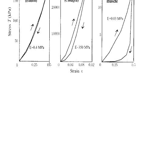
Figure 2: Elastin-rich canine nuchal ligament, collagen-rich sole tendon, and intestinal smooth muscle tensile properties. The sole tendon shows to be harder than the other two kinds of tissues, smaller the deformation biggest is the strain. In contrast, the intestinal smooth muscle shows to be more softness, strain value of $0.5$ is achieved with more facility than for nuchal ligament (elastin), it is also more viscoelastic than the others tissues, because it shows a wider hysteresis loop.

IV Soft Tissue Basic Properties

Once the biologic specimen is subjected to test methods as described above, their mechanical properties are obtained. In follow we describe more basic soft tissue mechanical properties.

IV.1 Inhomogeneous Structure

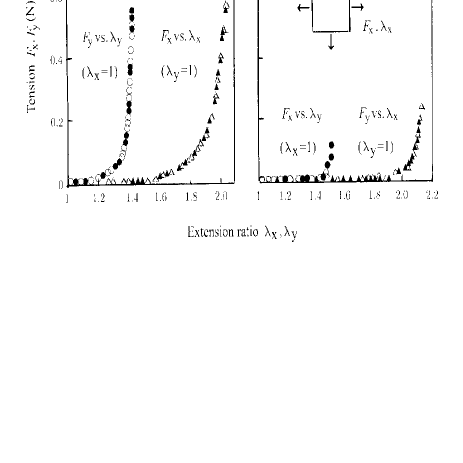
Figure 3: Tension-extension ratio relations of rabbit ventral skin. Different predetermined orthogonal directions are shown in the inset.

Biological soft tissues are mainly composed of cells and intercellular substances. The later consisting of connective tissues such as collagen, elastin and ground substance(hydrophilic gel). These components present different physical and chemical properties, and their contents differ from tissue to tissue and even from location to location within a tissue. Thus, mechanical properties depend both on tissue and on site.

Collagen is a protein which gives mechanical integrity and strength to our bodies, it is presented in different structural forms in different tissues and organs.

Elastin is also a protein, unlike to collagen has a much less integrated structure. It has much less strength and much more flexibility than collagen.

Figure ( 2) shows the stress-strain relationship for soft tissues rich in collagen, elastin and smooth muscle (cell)hasegawa . There we can see that, the elastin-rich nuchal ligament has much less strength and much more flexibility than the collagen-rich sole tendon, whereas the intestinal smooth muscle is much softer than the other soft tissues, which also shows a wider hysteresis loop; indicating that it is viscoelastic.

IV.2 Nonlinear Large Deformation and Anisotropy

Biological soft tissues are mechanically nonlinear, this is enhanced by assembly of structural component into a tissue. The behavior of arterial walls at low tension is similar to that of elastin, while the behavior at high tension is the same as that of collagen.

Collagen and elastin are long-chained polymers, so they are intrinsically anisotropic. In order to work effectively, not only their fibers but also cells are oriented in tissues and organs. Skin for example has very different properties in two orthogonal directions. This is shown in Figure ( 3), where extensions under different applied values of tension were measured. In this test method, Tension consists to subject the specimen to pre-determined value of force, i.e. $F_{x,y}$; the subindex recall for the direction, whereas the extension $\lambda_{x,y}$ is measured, taking the ratio of material length under the actual tension and its original one (when the tension is null). Note here that the sample achieves it original length when the tension value is zero.

Analogously, collagen fibers in the articular cartilage also shows anisotropic mechanical behaviortong . This is presented in Figure ( 4), where are shown different stress-strain curve responses for different orientations, i.e.$0,45,90$ degrees.

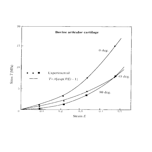
Figure 4: Tensile properties of bovine articular cartilage for different orientations. Here, we can also note certain nonlinear strain response of the soft tissue under stress.

IV.3 Viscoelasticity

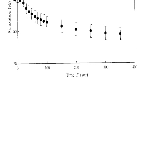
Figure 5: Relaxation behavior of rabbit patellar tendon

Most rheologist would restrict using of the label non-Newtonian fluid to substances which, because they possess long structural relaxation times, are non linear and tend to remember their past history. For almost all the biological soft tissues the curve stress-strain exhibit hysteresis loop, as it was shown in Figure ( 1) for elastin, collagen and soft muscle, meaning that they are viscoelastic. However, viscoelastic behavior is distinguished more clearly by relaxation test. For example, as it is shown in Figure ( 5), when the patellar tendon is elongated a given amount and the actual stress does not stay at a specific level but decreases rather rapidly at first and then graduallyyamamoto .

Generically speaking, under different strain rates (test speed) biological soft tissues are mechanically not very sensitive. In addition, the area of the hysteresis loop does not depend on the strain rate.

IV.4 Incompressibility

Most biological tissues hardly change their volume even if load is applied, so they are almost incompressiblechuong . They have a water content of more than 70 $\%$. However, articular cartilage is an exception, because is a micro-porous tissue, therefore water can enter an leave pores depending upon loadwoo .

The incompressibility assumption is a very important ingredient in constitutive laws formulation, imposing that adding overall principal strains is always zero.

V Mathematical Description of Mechanical Behavior

V.1 Tensile Behavior

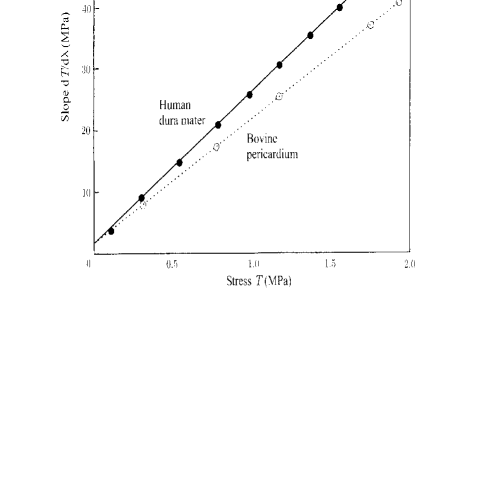
Figure 6: Slope of stress-extension ratio curve versus stress of human dura matter and bovine pericardium

Biological soft tissue can support large deformations which are nonlinear and extensive. In reducing the experimental data to a stress-strain relationship, it is used the nominal stress $\mathit{T}$ (getting dividing the force by the original cross sectional area specimen at zero stress). The most striking feature of this relationship is revealed in Figure ( 6) when the slope of the stress-extension curve is plotted against $\mathit{T}$. We can fit the experimental data to a straight line, as first approximation,

$$\frac{d\mathit{T}}{d\lambda}\,=\,B\,\mathit{T}\,+\,C\,,$$ (13)

where $\lambda$ is the extension ratio, $B$ and $C$ are constants depending of the material. Prescribed $\mathit{T}=0$, $\lambda=1$, from Eqn. ( 13) we obtain,

$$\mathit{T}\,=\,\frac{C}{B}\left\{\exp{\left[B\left(\lambda-1\right)\right]}\,-\,1\right\}\,.$$ (14)

Several other types of soft tissue such as the skin, the muscles, the ureter, the lung tissue, and articular cartilage are found to follow similar relationship, Figure ( 7). So, it appears that the exponential type of stress-strain relationship is common to biological tissue.

Realistically, in vivo tissues are not expose to such a pure tensile force conditions. Therefore, under more realistic mechanical conditions multi-axial test are often used to determine soft tissue mechanical behavior. So in several cases we need more equations. Naturally, for a three-dimensional organ we need a three-dimensional stress-strain law.

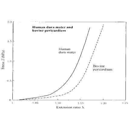
Figure 7: Stress-extension curves of human dura matter and bovine pericardium .

V.2 Multi-axial Behavior

No general constitutive equations has been identified for living tissues. Strain energy functions are used to describe the mechanical tissue properties. The main idea is that if a pseudo-elastic strain energy function exist, then the stress-strain relationship can be obtained by a differentiation. Let $\mathit{W}$ be the strain energy per unit mass of a tissue, and $\rho_{0}$ be the density in the zero-stress state. Thus $\rho_{0}\mathit{W}$ is the strain energy per unit volume of a tissue in the zero-stress state, this is called the strain-energy density function. The strain energy $\mathit{W}$ can be expressed in terms of the components $\mathit{E}_{ij}$ of the Green strain. In a uni-axial tensile test, the Green strain $\mathit{E}$ in the tensile direction is given by

$$\mathit{E}=E_{11}=\frac{1}{2}\left(\lambda^{2}-1\right)\,.$$ (15)

The components $\mathit{S}_{ij}$ of the second Piola-Kirchhoff stress can be obtained by derivatives of the strain energy density function,

$$\mathit{S}_{ij}=\frac{\partial\rho_{0}\mathit{W}}{\partial\mathit{E}_{ij}}\,.$$ (16)

In a simple uniaxial tensile test, the only non-zero component of stress, denoted by $\mathit{S}$, is

$$\mathit{S}=\mathit{S}_{11}=\frac{\mathit{F}}{\lambda\mathit{A}_{0}}\,,$$ (17)

where $\mathit{A}_{0}$ and $\mathit{F}$ are the initial cross-sectional area sample and the load applied to the specimen, respectively.

Equation ( 16) is a constitutive law or stress-strain relationship. Thus we need to know the details of the strain-energy functions. For the strain energy function, studies on non isotropic tissues as skin, muscles, ligaments, etc., have shown that the exponential form applies well. A general strain-energy function for biological soft tissues is given by Fung fung in the form

$$\begin{array}[]{ll}\mathit{W}&=\frac{1}{2}\alpha_{ijkl}\mathit{E}_{ij}\mathit{E}_{kl}+\left(\beta_{0}+\beta_{mnpq}\mathit{E}_{mn}\mathit{E}_{pq}\right)\\ &\times\mathit{exp}\left(\gamma_{ij}\mathit{E}_{ij}+\gamma_{ijkl}\mathit{E}_{ij}\mathit{E}_{kl}+\ldots\right)\,,\end{array}$$ (20)

where $\alpha_{jkl},\,\beta_{0},\,\beta_{mnpq},\,\gamma_{ij},\ldots$ are constants.

Regarded the complex form of Eqn. ( 20) high order terms can be dismissed as for skin, considered as being in a bi-axial state, and its strain-energy function is,

$$\begin{array}[]{ll}\rho_{0}\mathit{W}&=\frac{1}{2}\left(\alpha_{1}\mathit{E}^{2}_{11}+\alpha_{2}\mathit{E}^{2}_{22}+\alpha_{3}\mathit{E}^{2}_{12}+\alpha_{3}\mathit{E}^{2}_{21}+2\alpha_{4}\mathit{E}_{11}\mathit{E}_{22}\right)\\ &\frac{1}{2}c\,exp\left(a_{1}\mathit{E}^{2}_{11}+a_{2}\mathit{E}^{2}_{22}+a_{3}\mathit{E}^{2}_{12}+a_{3}\mathit{E}^{2}_{21}+2a_{4}\mathit{E}_{11}\mathit{E}_{22}+\gamma_{1}\mathit{E}^{3}_{11}+\gamma_{2}\mathit{E}^{3}_{22}+\gamma_{4}\mathit{E}^{2}_{11}\mathit{E}_{22}+\gamma_{5}\mathit{E}_{11}\mathit{E}^{2}_{22}\right)\,,\end{array}$$ (23)

where $\alpha_{1},\ldots,\alpha_{4},a_{1},\ldots\,a_{4},\gamma_{1},\ldots,\gamma_{5}$ and $c$ are constants.

Following, using Eqn. ( 16), we obtain the stresses,

$$\begin{array}[]{ll}\mathit{S}_{11}&=\frac{\partial\rho_{0}\mathit{W}}{\partial{E}_{11}}=\alpha_{1}\mathit{E}_{11}+\alpha_{4}\mathit{E}_{22}+c\mathit{A}_{1}\mathit{X}\,,\\ \mathit{S}_{22}&=\frac{\partial\rho_{0}\mathit{W}}{\partial{E}_{22}}=\alpha_{4}\mathit{E}_{11}+\alpha_{2}\mathit{E}_{22}+c\mathit{A}_{2}\mathit{X}\,,\\ \mathit{S}_{12}&=\frac{\partial\rho_{0}\mathit{W}}{\partial{E}_{12}}=\alpha_{3}\mathit{E}_{12}+c\,a_{3}\mathit{E}_{12}\mathit{X}\,,\end{array}$$ (27)

where $\mathit{A}_{1},\mathit{A}_{2}$ and $\mathit{X}$ are functions of the strain components.

It can be verified from Figure ( 3) that Eqn. ( 23) is suitable for bi-axial mechanical behavior of rabbit skin. Additional terms can be disregarded taking in account physical considerations, if we are concerned mainly with higher stresses and strains the first group of terms in Eqn. ( 23) can be omitted, in addition for practical purposes third order terms in the exponential function can also be omitted, and we have simply,

$$\rho_{0}\mathit{W}=\frac{1}{2}c\,exp\left(a_{1}\mathit{E}^{2}_{11}+a_{2}\mathit{E}^{2}_{22}+a_{3}\mathit{E}^{2}_{12}+a_{3}\mathit{E}^{2}_{21}+2a_{4}\mathit{E}_{11}\mathit{E}_{22}\right)\,.$$ (28)

V.3 Viscoelastic Behavior

Hysteresis, relaxation, and creep are common features of viscoelastic behavior for many materials. The toy models here presented are basic mechanical models useful describing viscoelastic behavior. These are composed by a combination of elastic material with elastic constant $\mu$ (i.e. spring) and a dashpot containing a fluid with coefficient of viscosity $\eta$. A force $F$ is suppose to produce on the spring an uniaxial linear deformation, denoted by the displacement $\mathit{u}$, and proportional to $\mu$. Whereas, at any instant, for the dashpot, it produces a velocity proportional to $\eta$. Different spring-dashpot arrangements are shown in Figure( 8).

It is remarkable that these classes of discrete models are also useful in the continuum, where relaxation functions are borrowed from these theories. For example modelling viscoelastic tissue behavior is assumed that the stresses in the material, which themselves may result from a nonlinear stress-strain relation are linearly superposed with respect to time, recalling the quasi-linear viscoelastic formulation, which we present next in subsection ( V.4).

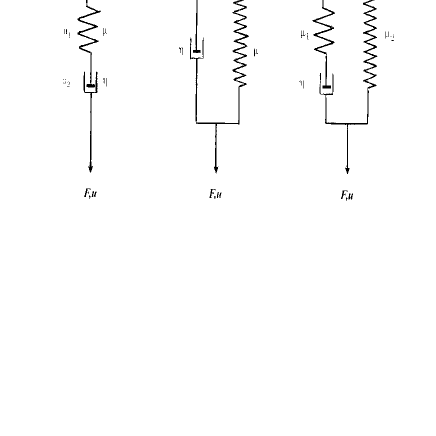
Figure 8: Spring-dashpot arranged as to describe different basic viscoelastic models.

V.3.1 Maxwell Model

In this model an spring and a dashpot are arranged in serie. Thus, the material behaves like an elastic at short time and it is viscous at long times.

$$\begin{array}[]{lr}\dot{\mathit{u}}=\dot{F}/\mu\,+\,F/\eta\,\,;&\mathit{u}(0)=\frac{F(0)}{\mu}\,.\end{array}$$ (30)

Equation ( 30) is solved, prescribed the force $F(t)$ is a unit step function, and the result is called the creep function $\mathit{c}(t)$. It represents the elongation produced by a sudden application of a constant unitary force at $t=0$,

$$c(t)=\left(\frac{1}{\mu}+\frac{1}{\eta}t\right)\mathbf{1}(t)\,.$$ (31)

Interchanging the role of $F$ and $\mathit{u}$, we obtain the relaxation function $\mathit{g}(t)$, as a response to a unity elongation, i.e. $\mathit{u}(t)=\mathbf{1}(t)$. The relaxation function is the force that must be applied to the specimen in order to produce an elongation, that changes at $t=0$ from zero to unity, remaining unity thereafter.

$$\mathit{g}(t)=\mu\,\exp{\left(-\mu{t}/\eta\right)}\,\mathbf{1}(t)\,,$$ (32)

with, 1(t) is the step function,

$$\mathbf{1}(t)=\left\{\begin{array}[]{ccl}1&;&t>0\,,\\ 1/2&;&t=0\,,\\ 0&;&t<0\,.\end{array}\right.$$ (36)

In this way, for the Maxwell model we found that a sudden application of a load induce an immediate deflection of the elastic spring, followed by a creep of the dashpot, as in Eqn. ( 31). On the other hand, a sudden deformation produces an immediate reaction by the spring followed by stress relaxation according to exponential law, which relaxation time is given by the factor $\eta/\mu$, as in Eqn. ( 32).

V.3.2 Voigt Model

Let us now regard the spring and the dashpot in parallel,

$$\begin{array}[]{lr}F=\mu\mathit{u}+\eta\,\dot{\mathit{u}}\,\,;&\,\mathit{u}(0)=0\,.\end{array}$$ (38)

Solving Eqn. ( 38) we obtain the creep and the stress relaxations functions, respectively,

$$\begin{array}[]{ccl}\mathit{c}(t)&=&\frac{1}{\mu}\left\{1-\exp{\left(-\mu\,t/\eta\right)}\right\}\mathbf{1}(t)\,,\\ \mathit{g}(t)&=&\eta\,\delta(t)+\mu\,\mathbf{1}(t)\,.\end{array}$$ (41)

Where, $\delta(t)$ is the Dirac delta function. Regarding Eqn. ( 41) we found that, a sudden application of a unity force will produce no immediate spring deflections; which solely built up gradually, because the dashpot arranged in parallel with the spring will not move instantaneously. The displacement of the dashpot will relax exponentially with a relaxation time $\eta/\mu$.

V.3.3 Kelvin Model

This model is also known as the Standard Linear model. While models due to Maxwell and Voigt suppose fluids behave like elastic to some extent, the standard model goes further taking in account the dissipation rate of energy in various materials subjected to cyclic loading,

$$\begin{array}[]{lr}F\,+\,\tau_{\epsilon}\,\dot{F}\,=\,E_{R}\left(\mathit{u}+\tau_{\sigma}\dot{\mathit{u}}\right)\,,&\tau_{\epsilon}\,F(0)\,=\,E_{R}\,\tau_{\sigma}\,\mathit{u}(0)\,.\end{array}$$ (43)

Here $\tau_{\epsilon}$ is the time of relaxation of the load under the condition of constant deflection, whereas $\tau_{\sigma}$ is the time of relaxation of deflection under the condition of constant load, and

$$\begin{array}[]{cc}\mathit{c}(t)&=\frac{1}{E_{R}}\left\{1-\left(1-\frac{\tau_{\epsilon}}{\tau_{\sigma}}\right)e^{-t/\tau_{\sigma}}\right\}\mathbf{1}(t)\,,\\ \mathit{g}(t)&=E_{R}\left\{1-\left(1-\frac{\tau_{\sigma}}{\tau_{\epsilon}}\right)e^{-t/\tau_{\epsilon}}\right\}\mathbf{1}(t)\,.\end{array}$$ (46)

In Eqn. ( 46) as $t\rightarrow\infty$, the dashpot is completely relaxed and the load-deflection relaxation becomes that of the springs, characterized by the constant $E_{R}$, which is called the relaxed elastic modulus.

V.3.4 Boltzmann Model

This is a most general formulation under the assumption of linearity between cause and effect. In the $1-\mathcal{D}$ case, analogously to the case above, we consider a bar subjected to a force $F(t)$ and an elongation $\mathit{u}(t)$. The elongation is caused by the total history of the loading up to the time $t$. Lets now consider an small time interval $d\tau$; at time $\tau$, the increment of loading is $\left(\frac{dF}{d\tau}\right)d\tau$ . It contributes an element $d\mathit{u}(t)$ to the elongation at time $t$, with a proportionality constant $c$, depending on the time interval $t-\tau$ , then,

$$\mathit{u}(t)=\int_{0}^{t}\mathit{c}(t-\tau)\,\frac{dF}{d\tau}\,d\tau\,.$$ (47)

Analogously, for the force,

$$F(t)=\int_{0}^{t}\mathit{g}(t-\tau)\,\frac{d\mathit{u}(\tau)}{d\tau}\,d\tau\,.$$ (48)

Here the functions $\mathit{c}(t-\tau)$ and $\mathit{g}(t-\tau)$ are the creep function and the relaxation function, respectively. More generally, we can write the relaxation function in the form,

$$\mathit{g}(t)=\sum_{n=0}^{N}\alpha_{n}\,e^{-t\nu_{n}}\,,$$ (49)

where $\nu_{n}=1/\tau_{n}$ is called characteristic frequency and $\alpha_{n}$ is an amplitude associated to each frequency $\nu_{n}$, it is called a spectrum of the relaxation function. A generalization to a continuum spectrum is giving in the next section.

V.4 Quasi-Linear Viscoelasticity of Biological Tissues

The hysteresis $\mathit{H}$ is due to viscoelasticity, it is defined as the ratio of the area of the hysteresis loop divided by the area under the loading curve. For biological tissues, $\mathit{H}$ is seen to be variable, but its variation with strain rate is not large, see Section ( IV.3). Hence, typical soft tissue behavior shows non-linearity of the stress-strain relationship and insensitivity of the material to strain rate.

Models due to Maxwell and Voigt provide a logarithmic type functional relationship between hysteresis and frequency ($\nu$, the inverse of the characteristic time), i.e., $\mathit{H}(\nu)\propto\,\ln(\nu)$. It is a decreasing curve for the former, whereas it is a increasing curve for the later. On the other hand, the Standard model presents a bell-shaped curve of hysteresis vs the logarithm of the frequency. Summarizing, none of these models present a typical flat hysteresis vs frequency curve of living tissues. However, this fact can be corrected by introducing nonlinear springs. Hence, this now suitable model for soft tissues, is composed of a long series of Kelvin bodies whose characteristic times ($1/\nu$) span a broad range.

Lets consider an elastic stress tensor $\mathit{T}^{(e)}$, which is a function of the strain tensor $\mathit{E}$. If the material is in the zero-stress state until the time $t=0$, then it is suddenly strained to $\mathit{E}$ and maintained constant at that value, thus the stress developed will be a function of time as well as of $\mathit{E}$. Hence, the history of the stress development may be written as,

$$\begin{array}[]{lr}\mathit{G}_{ijmn}(t)\mathit{T}_{mn}^{(e)}\mathit{(E)}\,;&\,\mathit{G}_{ijmn}(0)=1\,,\end{array}$$ (51)

in which $\mathit{G}_{ijmn}(t)$ is called the relaxation function, a normalized function of time. Now, we suppose that the stress response to an infinitesimal changes in a component of strain, $\delta\mathit{E}_{ij}$, superposed on a specimen in a state of strain $\mathit{E}$ at an instant of time $\tau$, is, for $t\,>\,\tau\,,$

$$\mathit{G}_{ijmn}(t-\tau)\,\frac{\partial\mathit{T}_{mn}^{(e)}\left[\mathit{E}(\tau)\right]}{\partial\mathit{E}_{ij}}\partial\mathit{E}_{ij}(\tau)\,.$$ (52)

In addition, assuming that the stress at time $t$ is the sum of the contributions of all the past changes,each governed by the same reduced relaxation function,

$$\mathit{T}_{ij}(t)=\int_{-\infty}^{t}\mathit{G}_{ijmn}(t-\tau)\,\frac{\partial\mathit{T}_{mn}^{(e)}[\mathit{E}(\tau)]}{\partial\mathit{E}_{kl}}\frac{\partial\mathit{E}_{kl}(\tau)}{\partial\tau}\,d\tau\,.$$ (53)

Although $\mathit{T}^{(e)}(\mathit{E})$ may be a nonlinear function of strain, the relaxation process is linear. Hence, this is a quasi-linear viscoelastic theory.

In particular, for the one-dimensional Kelvin model,

$$\mathit{G}(t)=\frac{1+\mathit{S}(q)\exp{\left(-t/q\right)}}{1+\mathit{S}(q)}\,,$$ (54)

with $q$ and $\mathit{S}(q)$ are constant parameters. The latter is called the relaxation spectrum and $1/q$ is a frequency. For an infinite number of Kelvin model in series, we can get the follow reduced relaxation function in the form,

$$\mathit{G}(t)=\frac{1+\int_{0}^{\infty}\mathit{S}(q)\exp{\left(-t/q\right)}\,dq}{1+\int_{0}^{\infty}\mathit{S}(q)\,dq}\,.$$ (55)

It has been shown that a specific spectrum, with constants $c,\,q_{1},\,q_{2}$, the follow function fits the data for the skin,arteries,ureter and teniae coli.

$$\mathit{S}(q)\left\{\begin{array}[]{ccc}c/q&;&\mbox{$q_{1}\leq\,q\leq\,q_{2}$}\,,\\ 0&;&\mbox{$q<q_{1}\,;q>q_{2}$}\,.\end{array}\right.$$ (58)

VI Vibrational Systems

In this section we suppose that a physical body is conformed by an ensemble of connected springs. Initially is being considered both spring elasticity and spring dumping responses are linear.

Hence, let us consider an elastic body obeying Hooke’s law. Let it be rigidly supported in a fixed space and subjected to a set of forces $\mathit{Q}_{i}$ acting at points $i\in\left(1,\ldots,n\right)$. Lets set up a generalized displacement $\mathit{q}_{i}$ at point $i$, in the direction of the force $\mathit{Q}_{i}$, be linearly proportional to the forces $\mathit{Q}_{1},\ldots,\mathit{Q}_{n}$, and vice versa, for $i\in\left(1,\ldots,n\right)$:

$$\begin{array}[]{ccccc}\mathit{q}_{i}=&\mathit{C}_{i1}\mathit{Q}_{1}&+\mathit{C}_{i2}\mathit{Q}_{2}&+\,...&+\mathit{C}_{in}\mathit{Q}_{n}\,,\\ \mathit{Q}_{i}=&\mathit{K}_{i1}\mathit{q}_{1}&+\mathit{K}_{i2}\mathit{q}_{2}&+\,...&+\mathit{K}_{in}\mathit{q}_{n}\,.\end{array}$$ (59)

The constants of proportionality $\mathit{C}_{ij},\mathit{K}_{ij}$ are independents of the forces and displacements. $\mathit{C}_{ij}$ are the flexibility influence coefficients and $\mathit{K}_{ij}$ are the stiffness influence coefficients, respectively. The physical meaning of $\mathit{K}_{ij}$ is the force required to act at the point $i$ due to a unit displacement at the point $j$, while another points (others than $j$) are held fixed. Analogously, $\mathit{C}_{ij}$ is the deflection at $i$ due to a unit force acting at $j$. The constraining equations ( 59) imply that exist a unique unstressed state to which the body return whenever all the external forces are removed, so the superposition principle applies. Moreover, it implies that the total work done by a set of forces does not depend of the order in which the forces are applied. This work done by each force is $\frac{1}{2}Q_{i}q_{i}$ and the total work done by the system of forces, is stored as strain energy in the elastic body , and it is given by,

$$\begin{array}[]{ll}\mathcal{U}&=\frac{1}{2}\sum_{i=1}^{n}\mathit{Q}_{i}\mathit{q}_{i}=\frac{1}{2}\sum_{i=1}^{n}\sum_{j=1}^{n}\mathit{K}_{ij}\mathit{q}_{i}\mathit{q}_{j}\,,\\ &=\frac{1}{2}\sum_{i=1}^{n}\sum_{j=1}^{n}\mathit{C}_{ij}\mathit{Q}_{i}\mathit{Q}_{j}\,.\end{array}$$ (62)

The matrices $\mathit{K}_{ij}$ and $\mathit{C}_{ij}$ are symmetric. In others words, the displacement at a point $i$ due to a unit force acting at another point $j$ is equal to the displacement at $j$ due to a unit force acting at $i$, i.e., they are positives in the same direction at each point.The stability of the system is guarantied if all the principal minors, including the determinant of the full $\mathit{K}_{ij}\,\,(\mathit{C}_{ij})$ matrices are positives.

Now we can write the equation of motions of a set o masses embedded in an elastic body. The D’Alambert’s principle establishes that the particles can be considered to be in a state of equilibrium if the inertial forces are applied in reversed direction on the particles. Thus, if the body is attached to a stationary support and we consider dumpers (lets said, dumping forces), then the dynamic equations written in vectorial form are

$$m_{i}\ddot{\mathit{q}}_{i}+\sum_{j=1}^{n}\mathit{K}_{ij}\mathit{q}_{j}+\sum_{i=1}^{n}\beta_{ij}\dot{\mathit{q}}_{j}\,=\,\mathit{F}_{i}^{e}\,;\left(i=1,\ldots\,n\right)\,.$$ (63)

Here $\mathit{q}_{i}$ is the displacement of the particle and $\mathit{F}^{e}_{i}$ is the external force acting on it.

However, damping force could be much more complex than this, for example it can be aerodynamics in origin, nonlinearly viscoelastic (as for tissues) and not necessarily stabilizing. For an immediate generalization of the theory, let recall for the concept of kinetic energy $\mathcal{K}$, it is an homogeneous quadratic function of the $\dot{\mathit{q}}$’s, and its rate can be computed from,

$$\dot{\mathcal{K}}=\sum_{i=1}^{n}\left(\frac{d}{dt}\frac{\partial\mathcal{K}}{\partial{\dot{\mathit{q}}}_{i}}-\frac{\partial\mathcal{K}}{\partial\mathit{q}_{i}}\right)\dot{q}_{i}\,.$$ (64)

For a biological system, other forms of energy rather than the kinetic energy $\mathcal{K}$ can also be involved, such as the gravitational potential $\mathcal{G}$, the internal energy $\mathcal{U}$, and the chemical energy $\mathcal{C}$. According to the first law of thermodynamics, the energy of a system solely can be changed by absorption of heat $\mathcal{H}$ and by doing work on the system. The rate of change of the total energy must be equal to the sum of the rates of heat input $\dot{\mathcal{H}}$ and work done on the system $\dot{\mathcal{W}}$, so,

$$\dot{\mathcal{K}}\,+\,\dot{\mathcal{G}}\,+\,\dot{\mathcal{U}}\,+\,\dot{\mathcal{C}}\,=\,\dot{\mathcal{H}}\,+\,\dot{\mathcal{W}}\,.$$ (65)

Generally, just a certain part of the internal energy function $\mathcal{U}$ arise from the strain energy, it is a quadratic function of (generalized) coordinates $q_{i}$. It can also depend on the temperature. If the temperature remains constant, then the rate at which work is done by the internal energy and also by the forces acting on a system are, respectively,

$$\begin{array}[]{lr}\dot{\mathcal{U}}\,=\,\sum_{i=1}^{n}\frac{\partial\mathcal{U}}{\partial\,q_{i}}\,\dot{q}_{i}\,;&\dot{\mathcal{W}}\,=\,\sum_{i=1}^{n}Q_{i}\,\dot{q}_{i}\,,\end{array}$$ (67)

then, substituting them into Eqn. ( 65),

$$\sum_{i=1}^{n}\left(\frac{d}{dt}\frac{\partial\mathcal{K}}{\partial\dot{q}_{i}}-\frac{\partial\mathcal{K}}{\partial\,q_{i}}+\frac{\partial\mathcal{U}}{\partial\,q_{i}}-Q_{i}\right)\dot{q}_{i}=\dot{\mathcal{H}}-\dot{\mathcal{G}}-\dot{\mathcal{C}}\,.$$ (68)

Now lets consider the special case when $\dot{\mathcal{H}}-\dot{\mathcal{G}}-\dot{\mathcal{C}}\equiv\,0\,.$ Because the displacements are independent variables, that can assume arbitrary variables, we impose for any $\dot{q}_{i}\neq\,0$, in Eqn. ( 68),

$$\frac{d}{dt}\frac{\partial\mathcal{K}}{\partial\dot{q}_{i}}\,-\,\frac{\partial\mathcal{K}}{\partial\,q_{i}}\,+\,\frac{\partial\mathcal{U}}{\partial\mathit{q}_{i}}\,=\,Q_{i}\,.$$ (69)

If the (generalized) forces are partial derivatives of a function, i.e., $Q_{i}=-\frac{\partial\mathcal{W}}{\partial\,q_{i}}$; where $\mathcal{W}$ is the potential energy. For the spring body system the internal elastic energy is given by Equation ( 62). Thought, $\mathcal{W}$ and $\mathcal{U}$ only depend on $\mathit{q}_{i}$, the system is conservative.

The aerodynamic or hydrodynamics forces acting on an animal moving in a fluid are not conservative. Hence, for problems involving these forces is much better to use Equation ( 69), thought $\mathit{Q}_{i}$ is an external force.

Following, we apply the present theory to materials showing viscoelastic behavior (like tissues), in the presence of fluid dynamic forces.

VI.1 Systems with Dumping and Fluid Dynamics Loads

Here we recall the most general constitutive equation of a linear viscoelastic solid reviewed in Section IV.3. Applying Boltzmann’s formulation we may write the internal force acting on a particle $i$, located at point $i$, by a displacement $\mathit{q}_{j}$ located at point $j$ as,

$$\mathit{F}_{ij}(t)=\int_{-\infty}^{t}\,G_{ij}(t-\tau)\frac{d\mathit{q}_{j}(\tau)}{d\tau}d\tau\,,$$ (70)

where $\mathit{G}_{ij}(t)$ are the relaxation functions. For solid with fading memory, it is given by equation ( 49),

$$\mathit{G}_{ij}(t)=\mathit{K}_{ij}+\beta_{ij}e^{-t\nu_{1}}+\,...\,+\gamma_{ij}e^{-t\nu_{n}}\,,$$ (71)

where $\nu_{1},\nu_{2},\,...\,,\nu_{n}$ are the relaxation frequencies , $K_{ij},\beta_{ij},\gamma_{ij}$ are spectral constants.

For systems subjected to fluid dynamics forces (i.e., in swimming, in wind or with internal flow), the external force at the point $i$ due to motion at point $j$ may be written as,

$$F_{ij}^{(e)}(t)=\int_{-\infty}^{t}\,A_{ij}(t-\tau)\frac{d\mathit{q}_{j}(\tau)}{d\tau}d\tau\,,$$ (72)

where $A_{ij}(t)$ are aerodynamic influence functions, which is un-symmetric.

Considering both the internal forces and a fluid dynamic forces given by Eqn.( 70) and Eqn. ( 72), Eqn. ( 69) can be rewritten as,

$$\begin{array}[]{ll}&m_{i}\frac{d^{2}\textit{q}_{i}(t)}{dt^{2}}+\sum_{j=1}^{n}\int_{-\infty}^{t}\mathit{G}_{ij}(t-\tau)\frac{d\textit{q}_{j}(\tau)}{d\tau}d\tau\\ &=\sum_{j=1}^{n}\int_{-\infty}^{t}\,A_{ij}(t-\tau)\frac{d\textit{q}_{j}(\tau)}{d\tau}d\tau+F_{i}^{(e)}\end{array}$$ (75)

where $F^{(e)}_{i}$ is the external force other than fluid dynamic forces.

VII Conclusions and Perspectives

More general mechanical properties of a material can be specified by mean of constitutive equations. Remarkable, the continuum approach naturally adds constitutive equations into more generalized theories. However, it seems that soft tissue models based on these more general theories are numerically expensive, hence that linear elasticity approaches have been preferentially considered.

On the other hand, spring-mass models present another alternative to model soft tissue mechanical behavior. Because of physical model simplicity and easier implementation, it has been preferentially used on applications for surgical simulations. The method is economic and fast, so it is a good candidate to operate in real time. However, until it is of our knowledge, its numerical implementation has been done no far away from the limits of linearity, not only regarding elasticity but even viscoelasticty.

In this work we have review some possible alternative models considering nonlinear elasticity and quasi-linear viscoelasticity on spring-mass models. The former can be naturally filling up by adding to the model exponential type deformations, as in section  V.1. Viscoelastic mechanical behavior can be added to the model using quasi linear models based on Boltzmann type approach, as shown in section  VI.1. Summarizing, these are the formulations we are going to explore in order to better model soft tissues. The resulting model will be validate by comparison with accurate models based on the continuum approach. We shall stress that because of simplicity and economy, this more elaborated spring-mass models can still handle to perform real time calculations.

Recently, Holzapfeld holzapfel3 and Ogden ogden2 have investigated numerical method based on the Continuum approach in order to regard nonlinear elasticity and Viscoelastic response on arterial walls and soft tissues. In addition to research for more sophisticated spring-mass models, these numerical methods are also going to pave the way of our research.

- (1) Ogden, R.W. (2001) Nonlinear Elasticity, Anisotropy, Material Stability and Residual Stress in Soft Tissue.
- (2) Holzapfel, G.A. (2000) Nonlinear Solid Mechanics. Chichester: Wiley.
- (3) Holzapfel, G. A. (2001) Biomechanics of Soft Tissue. In Lecture, J.ed., Handbook of Material Behavior Models. Boston: Academic Press 1049-63.
- (4) Bro-Nielsen, M. (1998). Finite Element Modelling in Surgery Simulation. Proc. of the IEEE: Special Issue on Virtual and Augmented Reality in Medicine 86 (3) 524-30.
- (5) Keeve, E., Girod, S., Pfeifel, P., Girod, B. (1996) Anatomy-Based Facial Tissue Modelling using the Finite Element Method. Proc. IEEE Visualization, San Francisco, CA. USA.
- (6) Koch, R.M., Gross, M.H., Bueren, D.F.,Franhauser, G., Parish, Y., Carls, F.R.(1996) Simulation Facial Surgery using Finite Element Modles. SIGGRAPH’96, ACM Computer Graphycs, August 30 .
- (7) Mosegaard, J. (2003). LR-Spring-mass Model for Cardiac Surgical Simulation. Medicine Meets Virtual Reality, (12) 256-58.
- (8) Teschrer, M., Girod, S., Girod, B. (2000). Direct Computation of Nolinear Soft-Tissue Deformation. Vison Modeling and Visualization VMV’000, Saarbucken, Germany, November 22-24.
- (9) Fung, Y.C. (1994) A first course in continuum mechanics. Prentice Hall, Englewood Cliff, New Yersey.
- (10) Hasegawa, M, and Azuna, T. (1974). Wall structure and static viscoelasticities of large veins. J. Jap. College Angiol. 14:87-92.
- (11) Tong, P. and Fung, Y.C. (1976). The stress-strain relationship for the skin. J. Biomech. 9:649-57.
- (12) Yamamoto, E., Hayashi, K. and Yamamoto, N. (1999). Mechanical properties of collagen fascicles from the rabit pattelar tendom. ASME J. Biomech. Eng. 121:124-31.
- (13) Chuong,C.J., and Fung,Y.C.(1984). Compressibility and Constitutive equation of arterial wall in radial compression experiments. J. Biomech, 17:35-40.
- (14) Woo, S.L.-Y., Lubock, P., Gomez, M.A.,Jemmott, G.F., Kuei, S.C. and Akeson, W.H.(1979) Large deformation nonhomogeneus and directional propertiesof articular cartilage. J. Biomech. 12:437-46.
- (15) Fung,Y.C.,Fronek,K. and Patitucci,P. (1979). Pseudoelasticity of arteries and the choice of its mathematical expression. Am. J. Physiol. 237:H620-631.
- (16) Holzapfel, G.A.,(2003). Structural and Numerical models for the (Visco)elastic Response of Arterial Walls with Residual Stresses, 109-184.International Centre for Mechanical Sciences. Springer, Wien, New Yersey.
- (17) Ogden, R.W.,(2003). Nolinear Elasticity, Anisotropy, Matyerial Stability and Residual Stress in Soft Tissue.Biomechanical of Soft Tussue in Cardiovascular Systems, 65-108. International Centre for Mechanical Sciences. Springer, Wien, New Yersey.