Game theoretic aspects of distributed spectral coordination with application to DSL networks

Abstract

In this paper we use game theoretic techniques to study the value of cooperation in distributed spectrum management problems. We show that the celebrated iterative water-filling algorithm is subject to the prisoner’s dilemma and therefore can lead to severe degradation of the achievable rate region in an interference channel environment. We also provide thorough analysis of a simple two bands near-far situation where we are able to provide closed form tight bounds on the rate region of both fixed margin iterative water filling (FM-IWF) and dynamic frequency division multiplexing (DFDM) methods. This is the only case where such analytic expressions are known and all previous studies included only simulated results of the rate region. We then propose an alternative algorithm that alleviates some of the drawbacks of the IWF algorithm in near-far scenarios relevant to DSL access networks. We also provide experimental analysis based on measured DSL channels of both algorithms as well as the centralized optimum spectrum management.

Keywords: Spectrum optimization, DSL, distributed coordination, game theory, interference channel.

I Introduction

Recent years have shown great advances in digital subscriber line (DSL) spectrum management. The public telephone copper lines network is limited by crosstalk between lines. As such dynamic management of the lines based on the actual crosstalk channels is becoming an important ingredient in enhancing the overall network performance at the physical layer. In a series of papers [13] [11], [8], [9] (and the references therein) Cioffi and his group defined several levels of spectral coordination for DSL access networks, where level zero coordination corresponds to no coordination, level one corresponds to distributed spectrum coordination, level two is centralized spectrum management where all spectral allocations are performed by a single spectrum management center (SMC). The third level is actually joint transmission / reception of all lines. To perform level three all signals are vectored into a single vectored signal. DSM level three can be divided into two types of vectoring: Two sided coordination (where all lines are both jointly encoded and jointly decoded) and single sided coordination where a central processing unit at the network side of the lines jointly encodes all the downstream transmission or jointly decodes the upstream transmissions. Two sided coordination is typical to private networks, and is implemented e.g., in gigabit Ethernet and the future 10 Gb Ethernet over copper. Single sided level three coordination is more relevant to public DSL networks where different lines are terminated at different customer houses. However joint transmission over all lines in a binder is still computationally complicated to implement due to several factors. First equipment already deployed uses the single input single output approach, where each line is operated independently assuming interference from other lines to be part of the background noise. Second the unbundling of the copper infrastructure and the deployment of remote terminals makes joint transmission impossible in certain scenarios. It is anticipated that fiber to the basement and fiber to the neighborhood architecture will benefit greatly from level three coordination, while legacy DSL deployment will not be enhanced by these techniques. On the other hand dynamic spectrum management (DSM) levels 1-2 only the power spectral density is optimized to enhance overall network performance is still an important tool for increasing the reach and improving the service of legacy long loops. The major difference between DSM level 1 and level 2 is the existence of a central spectrum management center performing the optimization jointly at level 2, while DSM level 1 requires distributed coordination of the lines, where each modem performs its optimization independently of the other lines. The most appealing property of level 1 coordination is the fact that it can be implemented using firmware upgrades to existing DSL modems (which already have a built in power spectral density (PSD) shaping capability), rather than complete replacement of infrastructure.

The basic approach to distributed coordination has been proposed in [8]. In this approach each modem is using the iterative waterfilling (IWF) algorithm to optimize its own spectrum. The modem iteratively optimizes its own transmit PSD against the actual noise caused by other modems in the binder. All modems repeat this process until convergence is achieved. There are three basic versions of the IWF algorithm [1]: Rate Adaptive (RA) where the modem uses all the power to maximize the rate, Margin Adaptive (MA) where excessive power is used to increase the margin and Fixed Margin (FM) where the modem minimizes the transmit power subject to a fixed margin and fixed rate constraint. This is done by reducing the power whenever the margin achieved is higher than required. This approach leads to great improvement over the totally selfish strategies of RA-IWF and MA-IWF. However as we shall demonstrate, large improvements can be achieved when the modems use a-priori agreed upon cooperative strategy.

Distributed coordination is basically a situation of conflict between the users. Each user would like to improve its rate even at the expense of other users. To gain some insight into the problem we apply game theoretic techniques. The distributed spectrum management process can be viewed as a game which is called the interference game [8]. In this game each user has a pay-off function given by its rate, and its strategies are basically choice of PSD. A fixed point of the IWF process is a Nash equilibrium in the interference game. However Nash equilibrium points can be highly suboptimal due to the well known Prisoner’s dilemma [7]. This suggests that defining a new cooperative game where players can commit to follow certain strategies will improve not only the overall network capacity, but also the individual user capacity (The payoff in the interference game is the achievable rate or capacity). A simple case of the interference game is the two users game. While this game is rather simplistic it captures well the interference environment between two groups of users: One group served from central office (CO) using legacy equipment such as ADSL or ADSL2+, and a second group served from a remote terminal (RT) over shorter lines and more modern equipment such as VDSL2 modems. It can also model well the case of two remote terminals of different service providers sharing customers in the same binder. These two cases are of great interest from practical point of view. Both cases influence the possible regulation of spectrum in an unbundled binder. Furthermore the case of remote terminals is crucial for maintaining legacy service integrity while expanding the network with remote terminals.

The rest of the paper is organized as follows: Section II formalizes the distributed spectrum coordination for Gaussian interference channel in terms of game theory. It is followed by Section III, in which the occurrence of the prisoner’s dilemma for a simplified symmetric two players game is analyzed. Section IV is devoted to the application of the previous results to the near-far problem in DSL channels. It provides analytic expression for the region where frequency division multiplexing will improve the rate region over the competitive IWF algorithm. In Section V we propose a simple dynamic frequency domain multiplexing (DFDM) scheme that can outperform the IWF in these cases. The results are also demonstrated on measured VDSL channels provided by France Telecom research labs (Section VI).

II The Gaussian interference game

In this section we define the Gaussian interference game, and provide some simplifications for dealing with discrete frequencies. For a general background on non-cooperative games we refer the reader to [7] and [6]. The Gaussian interference game was defined in [8]. In this paper we use the discrete approximation game. Let $f_{0}<\cdots<f_{K}$ be an increasing sequence of frequencies. Let $I_{k}$ be the closed interval be given by $I_{k}=[f_{k-1},f_{k}]$. We now define the approximate Gaussian interference game denoted by $GI_{\{I_{1},\ldots,I_{K}\}}$.

Let the players $1,\ldots,N$ operate over separate channels. Assume that the $N$ channels have crosstalk coupling functions $h_{ij}(k)$. Assume that user $i$’th is allowed to transmit a total power of $P_{i}$. Each player can transmit a power vector $\mbox{${\bf p}$}_{i}=\left(p_{i}(1),\ldots,p_{i}(K)\right)\in[0,P_{i}]^{K}$ such that $p_{i}(k)$ is the power transmitted in the interval $I_{k}$. Therefore we have $\sum_{k=1}^{K}p_{i}(k)=P_{i}$. The equality follows from the fact that in non-cooperative scenario all users will use the maximal power they can use. This implies that the set of power distributions for all users is a closed convex subset of the cube $\prod_{i=1}^{N}[0,P_{i}]^{K}$ given by:

$$\hbox{{\bf B}}=\prod_{i=1}^{N}\hbox{{\bf B}}_{i}$$ (1)

where $\hbox{{\bf B}}_{i}$ is the set of admissible power distributions for player $i$ is

$$\hbox{{\bf B}}_{i}=[0,P_{i}]^{K}\cap\left\{\left(p(1),\ldots,p(K)\right):\sum_{k=1}^{K}p(k)=P_{i}\right\}$$ (2)

Each player chooses a PSD $\mbox{${\bf p}$}_{i}=\left<p_{i}(k):1\leq k\leq N\right>\in\hbox{{\bf B}}_{i}$. Let the payoff for user $i$ be given by:

$$C^{i}\left(\mbox{${\bf p}$}_{1},\ldots,\mbox{${\bf p}$}_{N}\right)=\\ \sum_{k=1}^{K}\log_{2}\left(1+\frac{|h_{i}(k)|^{2}p_{i}(k)}{\sum|h_{ij}(k)|^{2}p_{j}(k)+\mbox{${\bf n}$}(k)}\right)$$ (3)

where $C^{i}$ is the capacity available to player $i$ given power distributions $\mbox{${\bf p}$}_{1},\ldots,\mbox{${\bf p}$}_{N}$, channel responses $h_{i}(f)$, crosstalk coupling functions $h_{ij}(k)$ and $n_{i}(k)>0$ is external noise present at the $i$’th channel receiver at frequency $k$. In cases where $n_{i}(k)=0$ capacities might become infinite using FDM strategies, however this is non-physical situation due to the receiver noise that is always present, even if small. Each $C^{i}$ is continuous on all variables.

Definition II.1

The Gaussian Interference game $GI_{\{I_{1},\ldots,I_{k}\}}=\left\{\hbox{{\bf C}},\hbox{{\bf B}}\right\}$ is the N players non-cooperative game with payoff vector $\hbox{{\bf C}}=\left(C^{1},\ldots,C^{N}\right)$ where $C^{i}$ are defined in (3) and B is the strategy set defined by (1).

The interference game is a special case of non-cooperative N-persons game. An important notion in game theory is that of a Nash equilibrium.

Definition II.2

An $N$-tuple of strategies $\left<\mbox{${\bf p}$}_{1},\ldots,\mbox{${\bf p}$}_{N}\right>$ for players $1,\ldots,N$ respectively is called a Nash equilibrium iff for all $n$ and for all ${\bf p}$ (${\bf p}$ a strategy for player $n$)

$$C^{n}\left(\mbox{${\bf p}$}_{1},...,\mbox{${\bf p}$}_{n-1},\mbox{${\bf p}$},\mbox{${\bf p}$}_{n+1},\ldots,\mbox{${\bf p}$}_{N}\right)<C^{n}\left(\mbox{${\bf p}$}_{1},...,\mbox{${\bf p}$}_{N}\right)$$

i.e., given that all other players $i\neq n$ use strategies $\mbox{${\bf p}$}_{i}$, player $n$ best response is $\mbox{${\bf p}$}_{n}$.

The proof of existence of Nash equilibrium in the general interference game follows from an easy adaptation of the proof of the this result for convex games. In appendix A we demonstrate how the continuity of the joint water-filling strategies is essentially what is needed in order to prove the existence of Nash equilibrium in the interference game. It is an adaptation of the result of [5] as presented in [6]. An alternative proof relying on differentiability has been given by Chung et.al [3]. A much harder problem is the uniqueness of Nash equilibrium points in the water-filling game. This is very important to the stability of the waterfilling strategies. A first result in this direction has been given in [2]. A more general analysis of the convergence (although it still does not cover the case of arbitrary channels has been given in [15].

While Nash equilibria are inevitable whenever non-cooperative zero sum game is played they can lead to substantial loss to all players, compared to a cooperative strategy in the non-zero sum case. In the next section we demonstrate this phenomena for a simplified channel model.

III The Prisoner’s Dilemma for the 2$\times$2 Symmetric Game

In order to present the benefits of cooperative strategies for spectral management we first focus on a simplified two users two frequency bands symmetric game. The channel matrices of this channel are the follows:

$$\left|H(1)\right|^{2}=\left[\begin{array}[]{cc}1&h\\ h&1\end{array}\right],\left|H(2)\right|^{2}=\left[\begin{array}[]{cc}1&h\\ h&1\end{array}\right]$$ (4)

where $H(1)$ and $H(2)$ are the normalized channel matrices for each frequency band, and

$$h=|h_{12}(1)|^{2}=|h_{21}(1)|^{2}=|h_{12}(2)|^{2}=|h_{21}(2)|^{2}$$

Since in the DSL environment the crosstalk from other user is smaller than the self channel response (i.e. $h_{ij}(k)<h_{i}(k)$ $\forall i,j,k$ we’ll limit the discussion to $0\leq h<1$.

In this section we analyze the symmetric $2\times 2$ interference game and find the Nash equilibrium which is achieved by both users using the full spectrum. We then provide full characterization of channel-SNR pairs for which IWF is optimal as well as full conditions for the two other situations: (in terms of pairs of channel coefficient and SNR) The first is known as the Prisoner’s dilemma (PD) and was discovered by Flood and Dresher [16]. The second is the “chicken” dilemma game, a termed coined by B. Russel in the context of the missile crisis in Cuba [17]. We will show that in both these cases cooperative strategies (FDM) outperform the Nash equilibrium achieved by the IWF.

In our symmetric game both users have the same power constraint $P$ and the power allocation matrix is defined as

$$P\cdot\left[\begin{array}[]{cc}1-\alpha&\alpha\\ \beta&1-\beta\end{array}\right]$$ (5)

The capacity for user I is as follows:

$$C^{1}=\frac{1}{2}\log_{2}\left(1+\frac{(1-\alpha)\cdot P}{N+\beta\cdot P\cdot h}\right)+\frac{1}{2}\log_{2}\left(1+\frac{\alpha\cdot P}{N+(1-\beta)\cdot P\cdot h}\right)$$ (6)

where $N$ is the noise power spectral density.
The last equation can be rewritten as -

$$C^{1}=\frac{1}{2}\log_{2}\left(1+\frac{(1-\alpha)}{SNR^{-1}+\beta\cdot h}\right)+\frac{1}{2}\log_{2}\left(1+\frac{\alpha}{SNR^{-1}+(1-\beta)\cdot h}\right)$$ (7)

where $SNR=P/N$.
By the definition of the Gaussian interference game, the set of strategies in this simplified game is

$$\left\{\alpha,\beta:0\leq\alpha,\beta\leq 1\right\}$$ (8)

Claim III.1

In the $2\times 2$ symmetric interference game there is Nash equilibrium point at $\alpha=\beta=\frac{1}{2}$.

Proof:

An IWF solution for this case will be of the form:

$$(1-\beta_{i-1})h+\alpha_{i}=\beta_{i-1}h+(1-\alpha_{i})$$ (9)

$$(1-\alpha_{i-1})h+\beta_{i}=\alpha_{i-1}h+(1-\beta_{i})$$ (10)

which implies that

$$\alpha_{i}=\frac{(2\beta_{i-1}-1)h+1}{2}$$ (11)

$$\beta_{i}=\frac{(2\alpha_{i-1}-1)h+1}{2}$$ (12)

The expression in (9) is the water filling solution for $\alpha$ in the $i^{th}$ iteration of the IWF as a function of $\beta$ computed in the $(i-1)^{th}$ iteration. Similarly (10) is the water filling solution for $\beta$ in the $i^{th}$ iteration as a function of $\alpha$ computed in the $(i-1)^{th}$ iteration. These set of equations will converges when

$$\alpha_{i}=\alpha_{i-1}\equiv\alpha$$ (13)

and

$$\beta_{i}=\beta_{i-1}\equiv\beta$$ (14)

substituting (13) and (14) in (11) and (12) and solving the two equations we get

$$\alpha=\beta=\frac{1}{2}$$ (15)

since the IWF converges to a Nash equilibrium we conclude that $\alpha=\beta=\frac{1}{2}$ is a Nash equilibrium in this game. ∎

We interpret the IWF as the competitive act, since each user maximizes its rate given the other user power allocation, we choose FDM as the cooperative way. Applying FDM (which implies that $\alpha=\beta=0$) means causing no interference to the other user ,by using orthogonal bands for transmission. We want to compare between these two approaches of power allocation, the competitive one (IWF) and the cooperative one (FDM). Instead of comparing these approaches on the ”continuous” game (continuous with respect to the set of strategies in the game defined in (8)), we can discuss and analyze the ”discrete” game, which is characterized by having only two strategies followed by a set of four different values of $\alpha$ and $\beta$. This reduction is allowed since for two strategies and two users there are four different choices of mutual power allocations:

• both users select FDM resulting in $\alpha=\beta=0$

• user I selects FDM while user II selects IWF resulting in $\alpha=0$ , $\beta=\frac{1-h}{2}$ ($\beta$ is the solution of 12 where $\alpha=0$)

• user I selects IWF while user II selects FDM resulting in $\alpha=\frac{1-h}{2}$ , $\beta=0$ ($\alpha$ is the solution of 11 where $\beta=0$)

• both users select IWF resulting in $\alpha=\beta=\frac{1}{2}$ as we have shown in the theorem

Tables I describes the payoffs of users I at four different levels of mutual cooperation (The payoffs of user II are the same with the inversion of the cooperative/competetive roles).

TABLE I: User I payoffs at different levels of mutual cooperation

	user II is fully cooperative	user II is fully competing
	$(\beta=0)$	$\left(\beta=\frac{(2\alpha-1)h+1}{2}\right)$
$\begin{array}[]{c}$user I is fully cooperative$\\ (\alpha=0)\end{array}$	$\frac{1}{2}\log_{2}\left(1+\frac{1}{SNR^{-1}}\right)$	$\frac{1}{2}\log_{2}\left(1+\frac{1}{SNR^{-1}+\frac{(1-h)}{2}h}\right)$
$\begin{array}[]{c}$user I is fully competing$\\ \left(\alpha=\frac{(2\beta-1)h+1}{2}\right)\\ \end{array}$	$\frac{1}{2}\log_{2}\left(1+\frac{\frac{1+h}{2}}{SNR^{-1}}\right)+\frac{1}{2}\log_{2}\left(1+\frac{\frac{1-h}{2}}{SNR^{-1}+h}\right)$	$\log_{2}\left(1+\frac{\frac{1}{2}}{SNR^{-1}+\frac{1}{2}h}\right)$

For certain values of the payoff (determined by channel and SNR) in the interference game it might be the case that each user can benefit from other players cooperation, and benefit even more from mutual cooperation. However it is always the case that given cooperative strategy for the other player he always benefits from noncooperation with the others due to the water filling optimality (i.e. given the interference and noise PSD the best way to allocate the power is through water filling which, as before mentioned, don’t take into account the influence on other users thus cannot be considered as a cooperative method). In this situation the stable equilibrium is the mutual non-cooperation. If on the other hand mutual cooperation is better for both users over mutual competition we obtain that the stable point is suboptimal for both players. This is a well known situation in game theory termed the Prisoner’s Dilemma [7] (here and after abbreviated PD). For a popular overview of the prisoner’s dilemma as well as other basic notions in game theory as well as history of the subject we recommend [17].

A PD situation is defined by the following payoff relations - $T>R>P>N$, where:

• $T$ (Temptation) is one’s payoff for defecting while the other cooperates. In our game choosing an IWF while the other player uses FDM.

• $R$ (Reward) is the payoff of each player where both cooperate or mutual choice of FDM.

• $P$ (Penalty) is the payoff of each player when both defects or mutual use of IWF.

• $N$ (Naive) is one’s payoff for cooperating while the other defects, i.e., the result of using FDM when the other player uses IWF.

It is easy to show that the Nash equilibrium point in this case is that both players will defect ($P$). This is caused by the fact that given the other user act the best response will be to defect (since $T>R$ and $P>N$). Obviously a better strategy (which makes this game a dilemma) is mutual cooperation (since $R>P$).

In our symmetric interference game $\alpha$ and $\beta$ can be viewed as the level of mutual cooperation. $\alpha$ determines the level and cooperation of user I with user II, and $\beta$ the level of cooperation of user II with user I. For analyzing this game we can analyze the simplified discrete game. As before mentioned a PD situation is characterized by the following payoff relations: $T>R>P>N$. By examining the relations between the different rates (payoffs) as depicted in table I we can derive a set of conditions on $h$ and $SNR$ for which the given symmetric interference channel game defines a PD situation:
(a) $T>R$:

$$\frac{1}{2}\log_{2}\left(1+\frac{\frac{1+h}{2}}{SNR^{-1}}\right)+\frac{1}{2}\log_{2}\left(1+\frac{\frac{1-h}{2}}{SNR^{-1}+h}\right)>\frac{1}{2}\log_{2}\left(1+\frac{1}{SNR^{-1}}\right)$$ (16)

this equation reduces to $h^{2}-2\cdot h+1>0$ which holds for every $h\neq 1$.

(b) $T>P$:

$$\frac{1}{2}\log_{2}\left(1+\frac{\frac{1+h}{2}}{SNR^{-1}}\right)+\frac{1}{2}\log_{2}\left(1+\frac{\frac{1-h}{2}}{SNR^{-1}+h}\right)>\log_{2}\left(1+\frac{\frac{1}{2}}{SNR^{-1}+\frac{1}{2}h}\right)$$ (17)

simplifying the equation we obtain

$$SNR^{-2}\left(h+\frac{1}{4}h^{2}\right)+SNR^{-1}\left(\frac{1}{2}h^{3}+\frac{3}{4}h^{2}+\frac{1}{4}h\right)+\left(\frac{1}{16}h^{4}+\frac{1}{8}h^{3}+\frac{1}{16}h^{2}\right)>0$$ (18)

since $SNR$ and $h$ are nonnegative the equation always true.

(c) $R>P$

$$\frac{1}{2}\log_{2}\left(1+\frac{1}{SNR^{-1}}\right)>\log_{2}\left(1+\frac{\frac{1}{2}}{SNR^{-1}+\frac{1}{2}h}\right)$$ (19)

simplifying (15) we get

$$h^{2}+2hSNR^{-1}-SNR^{-1}>0$$ (20)

since $h$ is nonnegative the equation holds for $h>h_{\lim 1}$, where

$$h_{\lim 1}=SNR^{-1}\left(\sqrt{1+\frac{1}{SNR^{-1}}}-1\right)$$ (21)

(d) $R>N$

$$\frac{1}{2}\log_{2}\left(1+\frac{1}{SNR^{-1}}\right)>\frac{1}{2}\log_{2}\left(1+\frac{1}{SNR^{-1}+\frac{(1-h)}{2}h}\right)$$ (22)

which reduces to $\frac{1-h}{2}\cdot h>0$, this equation holds for every $0\leq h<1$.
(e) $P>N$

$$\log_{2}\left(1+\frac{\frac{1}{2}}{SNR^{-1}+\frac{1}{2}h}\right)>\frac{1}{2}\log_{2}\left(1+\frac{1}{SNR^{-1}+\frac{(1-h)}{2}h}\right)$$ (23)

or equivalently

$$h^{3}+h^{2}(0.5+2SNR^{-1})-0.5h-SNR^{-1}<0$$ (24)

since $h$ is nonnegative the equation holds for $h<h_{\lim 2}$, where $h_{\lim 2}$ is the solution for (24) given by the cubic formula. Another condition arises from the sum-rate perspective is the following - $2R>T+N$. This condition implies that a mixed strategy (i.e. one user is cooperating while the other competing) will not achieve higher sum rate than mutual cooperation -
(f) $2R>T+N$:

$$\log_{2}\left(1+\frac{1}{SNR^{-1}}\right)>\frac{1}{2}\log_{2}\left(1+\frac{\frac{1+h}{2}}{SNR^{-1}}\right)+\frac{1}{2}\log_{2}\left(1+\frac{\frac{1-h}{2}}{SNR^{-1}+h}\right)+\frac{1}{2}\log_{2}\left(1+\frac{1}{SNR^{-1}+\frac{(1-h)}{2}h}\right)$$ (25)

which reduced to

$$SNR^{-2}\left(6(1-h^{2})+8h\right)+SNR^{-1}(9h+h^{2})+4h^{2}(1-h)>0$$ (26)

since $h$ and $SNR$ are nonnegative the equation is true in the relevant region of $0\leq h<1$ for every $SNR$. Combining all the relation above we conclude that only three situation are possible:

• (A) $T>P>R>N$ , for $h<h_{\lim 1}$

• (B) $T>R>P>N$ , for $h_{\lim 1}<h<h_{\lim 2}$

• (C) $T>R>N>P$ , for $h_{\lim 2}<h$

where $h_{\lim 1}$ and $h_{\lim 2}$ are given above.
The sum rate is either $2\cdot R$ (when both applying FDM), $2\cdot P$ (when both using IWF) or $T+N$ (when one uses IWF while the other applying FDM). Examining the achieved sum rate for the two strategies (IWF and FDM) yields the following: The payoff relations in (A) corresponds to a game called ”Deadlock”. In this game there is no dilemma, since as in the PD situation, no matter what the other player does, it is better to defect ($T>R$ and $P>N$), so the Nash equilibrium point is $P$. However in contrast to PD, in this game $P>R$ thus there is no reason to cooperate. The maximum sum rate is also $P$ because $2\cdot R>T+N$ and $P>R$. Since applying the IWF strategy equals to $P$ (by our definition of competition), this is the region where the IWF algorithm achieves the maximum sum rate as well as optimal rate for each user.

The payoff relations in (B) corresponds to the above discussed PD situation. While the Nash equilibrium point is $P$, the maximum sum rate is achieved by $R$. In this region the FDM strategy will achieve the maximum sum rate.

The last payoff relations (C) corresponds to a game called ”Chicken”. This game has two distinguished Nash equilibrium points, $T$ and $N$. This is caused by the fact that for each of the other player’s strategies the opposite response is preferred (if the other cooperates it is better to defect since $T>R$, while if the other defects it is better to cooperate since $N>P$). The maximum rate sum point is still at $R$ (since $R>P$ and $2\cdot R>T+N$) thus, again FDM will achieve the maximum rate sum while IWF will not.

An algorithm for distributed power allocation can be derived from this insight for the symmetric interference game. Given a symmetric interference game (i.e. a symmetric channel matrix and $SNR$), if $h<h_{\lim 1}$ (where $h_{\lim 1}$ is given in (21)) use the IWF method to allocate the power, else, both players should use the FDM method. Since the channel crosstalk coefficient $h$ is assumed to be known to both users this algorithm can be implemented distributively (with pre agrement on the band used by each user for the FDM). We will return to this strategy in the context of real DSL channels in section V

It is important to distinguish between the continuous symmetric interference game and the discrete one. Even though the discrete game can have Nash equilibrium other than $\alpha=\beta=\frac{1}{2}$ (as we saw in the chicken game) these equilibrium points are not stable in the continuous game. Hence we are left with only one stable equilibrium as proven in (III.1). Nevertheless, our conclusions regarding the benefit of cooperation in the interference game derived from the discrete game remains valid in the continuous one since once continuous strategies are chosen they inevitably lead to $\alpha=\beta=0.5$. However when players choose to cooperate the stability issue is not important since IWF is not used.

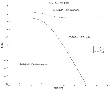
Figure 1: Graph of $h_{\lim 1}$ , $h_{\lim 2}$ Vs. SNR, The solid line corresponds to $h_{\lim 1}$ and the dashed line corresponds to $h_{\lim 2}$

Further discussion and examples of the prisoner’s dilemma in this case can be found in [20].

IV The Near-Far Problem

One of the most important spectral coordination problems in the DSL environment is the near-far problem. This problem has similarity to the power control problem in CDMA network. However the DSL channel is frequency selective (see Figure 2) and multi-carrier modulation is typically used. Therefore the interference from remote terminal to CO based services is very severe and has properties similar to near end crosstalk (NEXT). This scenario is typical to unbundled loop plants where the incumbent operator is mandated by law to lease CO based lines to competitive operators. Figure 2 describes a typical near far interference environment.

The problem has also appeared in the upstream direction of VDSL (which is at frequencies above 3MHz). The solution of the VDSL standard is highly suboptimal since the optimization has been done for fixed services under specific noise scenarios. It has been shown that upstream spectral coordination can lead to significant enhancement of upstream rates in real life environments. While DSL channels have relatively complicated frequency response and full analysis is possible only based on computer simulations and measured channels, we provide here an analysis of a simplified near far scenario that captures the essence of distributed cooperation in near far scenarios. In section VI we will provide simulated experiments on measured channels.

The analysis in this section is divided into two parts. First a simple symmetric bandwidth near-far game with no option to partition the bands is analyzed and it is proved that an FDM solution is optimal. Then the results are extended to a more general situation with asymmetric bandwidth. In this case we show that a solution minimizing the interference by utilizing only part of the band is preferable to a global FM-IWF. This is done by providing analytic bounds on the rate region for both strategies. Unlike all previous analysis of these strategies we are able to provide analytic bounds on the rate region.

IV-A Symmetric two bands Near-Far problem

Consider the case of two users using two bands with channel matrices given by

$$\left|H(1)\right|^{2}=\left[\begin{array}[]{cc}\alpha&\beta\\ \gamma&1\end{array}\right],\left|H(2)\right|^{2}=\left[\begin{array}[]{cc}0&\delta\\ \varepsilon&1\end{array}\right]$$ (27)

where $H(1)$ and $H(2)$ are the normalized channel matrices for each frequency band. Note that the second band can be used only by the second user which will be termed the strong user. Furthermore we assume that the first band can be used partly by the second user if he chooses a non-naive FDM or non-naive TDM strategies. The first user will be called the weak user. To simplify the discussion we make the following assumptions:

• Both users have transmit power limitation $P$. This is not essential but simplifies notation.

• $\alpha<<1$ This is the reason that we refer to the first user as the weak user.

• $N_{i}$ is the additive Gaussian noise is constant for both receivers and at both bands. This assumption is reasonable since the design of all multi-carrier modems requires low modem noise floor in order to support the high constellations.

• $N_{i}<<\beta P$ This means that the weak user is limited by the crosstalk from the strong user.

• $\gamma P<<N_{i}<<0.5P$. Typically the weak lines emerging from the CO generate crosstalk that is negligible into the RT line. This means that basically the strong user sees the same signal to noise ratio across the two bands. This is actually better for the weak user than the real situation where the strong user observes better SNR on the first band. The second inequality suggest that we work in the bandwidth limited high SNR regime, which is the interesting case for DSL networks.

• User II can perform a voluntary power backoff $\tau$.

Under our assumptions user II completely dominates the achievable rate of user I, and user I has no way to force anything on user II. This type of game is called “The Bully” game, where the strong user can decide to behave in any manner. We would like to analyze the benefits of a “polite bully” that takes whatever it needs, but behaves as polite as possible to other users, by allowing them to use resources he does not need.

To that end we analyze the capacity region of the two users under water-filling strategies and under interference minimization strategy of the second user, where the strong user utilizes only partially the joint resource which is the first band. Note that all the strategies are purely distributed since only the agreement to behave politely by the bully player is required. We make several observations regarding the possible strategies:

Claim IV.1

The weak user will always use all its power in the first band.

This claim follows from the fact that user I has no capacity in the second band.

Let the power allocation of user II be $\left(P_{1},P_{2}\right)$ such that $P_{1}+P_{2}=P$.

Claim IV.2

The rate achievable by user I is given by

$$C^{1}=\log_{2}\left(1+\frac{\alpha P}{\beta P_{1}+N_{1}}\right)$$

This claim is implied by our assumptions of Gaussian signalling by both users and independent detection of each user. Typically for the DSL interference channel, the interference to AWGN ratio is insufficient for successive interference cancelation so each user should treat the other users interference as Gaussian noise. It is now easy to compute the optimal rate adaptive strategy for user II.

Claim IV.3

The power allocation for user II under politeness factor $\tau$ is given by

$$\begin{array}[]{lcl}P_{1}=\frac{P}{2}(\tau-\gamma)&&P_{2}=\frac{P}{2}(\tau+\gamma)\end{array}$$ (28)

The proof for claim IV.3 follows the same lines as the proof of claim III.1. The WF solution suggests a constant level of the transmitted power + noise (which includes the interference) for each band. In our case this implies that

$$P_{1}+N_{2}+\gamma P=P_{2}+N_{2}$$ (29)

since $P_{1}+P_{2}=\tau P$ we can rewrite the equation as

$$2P_{1}+\gamma P=\tau P.$$ (30)

Solving for $P_{1}$ we obtain $P_{1}=\frac{P}{2}(\tau-\gamma)$ and $P_{2}=\frac{P}{2}(\tau+\gamma)$ We now obtain the rate for user II.

Claim IV.4

The rate of user II under FM-IWF with power backoff $\tau$ is given by:

$$C^{2}=\log_{2}\left(1+\frac{P_{1}}{N_{2}+\gamma P}\right)+\log_{2}\left(1+\frac{P_{2}}{N_{2}}\right)$$ (31)

where $P_{1}$ and $P_{2}$ are given by (28).

An alternative approach for user II can be to minimize the interference to the first band by increasing the power in the second band should it find it useful. This leads to different expression for the capacity region.

The expression for the capacities using the cooperative act of user II have the same form as before

$$\begin{array}[]{c}C^{1}=\log_{2}\left(1+\frac{\alpha P}{N_{1}+\beta\tilde{P_{1}}}\right)\\ C^{2}=\log_{2}\left(1+\frac{\tilde{P_{1}}}{N_{2}+\gamma P}\right)+\log_{2}\left(1+\frac{\tilde{P_{2}}}{N_{2}}\right)\end{array}$$ (32)

Where $(\tilde{P_{1}},\tilde{P_{2}})$ is the new power allocation of user II such that $\tilde{P_{1}}+\tilde{P_{2}}=\tilde{\tau}P$

In order to find the $(\tilde{P_{1}},\tilde{P_{2}})$ we need to choose the minimal $\tilde{P_{1}}$ such that the following equation holds

$$\log_{2}\left(1+\frac{P_{1}}{N_{2}+\gamma P}\right)+\log_{2}\left(1+\frac{P_{2}}{N_{2}}\right)=\log_{2}\left(1+\frac{\tilde{P_{1}}}{N_{2}+\gamma P}\right)+\log_{2}\left(1+\frac{\tilde{P_{2}}}{N_{2}}\right)$$ (33)

where $P_{1},P_{2}$ are defined by (28). It is clear that in order to minimize $\tilde{P_{1}}$ we need to set $\tilde{\tau}$ to 1. By doing so we enable user II to allocate the maximum amount of power on the second band and therefor minimize the power on the first band. Substituting $\tilde{P_{2}}$ with $P-\tilde{P_{1}}$ and solving (33) for $\tilde{P_{1}}$ we get

$$\tilde{P_{1}}=\frac{1}{2}P(1-\gamma)\pm\frac{1}{2}\left[P(1-\tau)(P+4N_{2}+2\gamma P+P\tau)\right]^{\frac{1}{2}}$$ (34)

Using the minimal solution for $\tilde{P_{1}}$ and applying some algebra on the expression above we obtain

$$\tilde{P_{1}}=\frac{1}{2}P(1-\gamma)-\frac{1}{2}\left[P^{2}(1-\tau)^{2}\left(\frac{1+4N_{2}/P+2\gamma+\tau}{1-\tau}\right)\right]^{\frac{1}{2}}$$ (35)

which can be rewritten as

$$\tilde{P_{1}}=\frac{1}{2}P(1-\gamma)-\frac{1}{2}P(1-\tau)\left(\frac{1+4N_{2}/P+2\gamma+\tau}{1-\tau}\right)^{\frac{1}{2}}$$ (36)

Since the term $\left(\frac{1+4N_{2}/P+2\gamma+\tau}{1-\tau}\right)$ is grater or equal to 1 the square root of this term is also grater or equal to 1. We can write

$$1+\Delta=\sqrt{\frac{1+4N_{2}/P+2\gamma+\tau}{1-\tau}}$$

where $\Delta$ is some positive constant. Therefore we can write

$$\tilde{P_{1}}=\frac{1}{2}P(1-\gamma)-\frac{1}{2}P(1-\tau)(1+\Delta)$$ (37)

arranging (37) we get

$$\tilde{P_{1}}=\frac{1}{2}P(\tau-\gamma)-\frac{1}{2}P(1-\tau)\Delta$$ (38)

which, by claim IV.3 becomes

$$\tilde{P_{1}}=P_{1}-\frac{1}{2}P(1-\tau)\Delta$$ (39)

If the value of $\tilde{P_{1}}$ as given in (39) is negative we should fix it to zero. This is the best situation for user I as he sees no interference at all.

Since $C^{2}$ is equal for both methods (guaranteed by (33)) and $\tilde{P_{1}}\leq P_{1}$ (i.e. the interference that user I sees using the cooperative method is less than or equal to the one obtained by FM IWF) we conclude that the rate region achieved using the cooperative act contains the rate region related to FM IWF.

IV-B Near-Far problem in the bandwidth limited case

Our next step will be to extend the analysis above to the case where the two bands have non-identical bandwidth, and we work in the bandwidth limited regime, i.e., the spectral efficiency of the transmission is higher than 1 (we transmit more than 1 bit per channel use). In this case the signal to noise ratio at each receiver is positive. This will capture a more realistic ISI limited channel similar to the DSL channel. We shall restrict the analysis to flat attenuation in each band.

Assume that the first band has bandwidth $W_{1}$ and the second band has bandwidth $W_{2}$. Similarly to the previous case assume that the channel matrices at each band are given by (27).

To simplify the expressions we shall also assume that $\gamma P<<N_{2}W_{i}$, where $N_{2}$ is the PSD of the AWGN of the second user receiver. This is realistic in typical near far problems in DSL where the FEXT from the CO lines into the RT lines is negligible compared to the AWGN due to the strong loop attenuation of lines originating at the CO. Under our assumptions we prove the following:

Theorem IV.1

The rate region of the FM-IWF satisfies

$$W_{1}\log_{2}\left(1+\frac{\alpha P}{\beta P\left(2^{\frac{R_{2}}{W_{1}+W_{2}}-1}\right)/{\bar{\hbox{SNR}}}_{2}+W_{1}N_{1}}\right)\leq R_{1}\leq W_{1}\log_{2}\left(1+\frac{\alpha P}{\beta P\left(2^{\frac{R_{2}}{W_{1}+W_{2}}+1}\right)/{\bar{\hbox{SNR}}}_{2}+W_{1}N_{1}}\right)$$ (40)

where $\rho=\frac{W_{1}}{W1+W_{2}}$ and

$${\bar{\hbox{SNR}}}_{2}=\left(\frac{P}{N_{2}W_{1}}\right)^{\rho}\left(\frac{P}{N_{2}W_{2}}\right)^{1-\rho}$$ (41)

is a generalized geometric mean of the SNR at the two bands.

The capacity of the two users is now given by:

$$\begin{array}[]{c}C^{1}=W_{1}\log_{2}\left(1+\frac{\alpha P}{N_{1}W_{1}+\beta{P_{1}}}\right)\\ C^{2}=W_{1}\log_{2}\left(1+\frac{{P_{1}}}{N_{2}W_{1}+\gamma P}\right)+W_{2}\log_{2}\left(1+\frac{{P_{2}}}{N_{2}W_{2}}\right)\end{array}$$ (42)

where again $P_{1}+P_{2}=\tau P$. To determine $\tau$ assume that the target rate of the bully player is $R_{2}$ and ignore $\gamma P$ by our assumption. Therefore IWF results in flat transmit PSD for user 2:

$$\begin{array}[]{l}P_{1}=\rho\tau P\\ P_{2}=(1-\rho)\tau P\end{array}$$

We require that

$$R_{2}=W_{1}\log_{2}\left(1+\frac{{\rho\tau P}}{N_{2}W_{2}}\right)+W_{2}\log_{2}\left(1+\frac{(1-\rho)\tau P}{N_{2}W_{2}}\right)$$ (43)

Therefore we obtain

$$R_{2}\geq W_{1}\log_{2}\left(\frac{{\rho\tau P}}{N_{2}W_{1}}\right)+W_{2}\log_{2}\left(\frac{(1-\rho)\tau P}{N_{2}W_{2}}\right)$$ (44)

Actually using the high SNR approximation we can replace the inequality by approximate equality. Hence

$$2^{R_{2}}\geq\left(\frac{\rho\tau P}{N_{2}W_{1}}\right)^{W_{1}}\left(\frac{(1-\rho)\tau P}{N_{2}W_{2}}\right)^{W_{2}}$$ (45)

Hence

$$2^{\frac{R_{2}}{W_{1}+W_{2}}}\geq\left(\frac{\rho\tau P}{N_{2}W_{1}}\right)^{\rho}\left(\frac{(1-\rho)\tau P}{N_{2}W_{2}}\right)^{1-\rho}$$ (46)

Further simplification yields

$$2^{\frac{R_{2}}{W_{1}+W_{2}}}\geq\frac{\tau P}{N_{2}W_{1}^{\rho}W_{2}^{1-\rho}}\rho^{\rho}(1-\rho)^{(1-\rho)}$$ (47)

Therefore

$$\tau\leq\frac{2^{\frac{R_{2}}{W_{1}+W_{2}}}}{{\bar{\hbox{SNR}}}_{2}\rho^{\rho}(1-\rho)^{(1-\rho)}}$$ (48)

Also note that since $0<\rho<1$

$$\frac{1}{2}\leq\rho^{\rho}(1-\rho)^{(1-\rho)}\leq 1$$

hence

$$\tau\leq\frac{2^{\frac{R_{2}}{W_{1}+W_{2}}+1}}{{\bar{\hbox{SNR}}}_{2}}$$ (49)

Substituting (49) into (42) we obtain that the rate for user I is bounded by

$$R_{1}\leq W_{1}\log_{2}\left(1+\frac{\alpha P}{\beta P\left(2^{\frac{R_{2}}{W_{1}+W_{2}}+1}\right)/{\bar{\hbox{SNR}}}_{2}+W_{1}N_{1}}\right)$$ (50)

This is indeed very satisfying. As we know the bully’s power backoff is determined by the required spectral efficiency $R_{2}/(W_{1}+W_{2})$ and the geometric mean SNR of the bully player. Also note that no matter how good the SNR of user II on the second band, the FM-IWF always incurs a loss to user I’s capacity, since there is always additional disturbance in the first band. The total rate can be rewritten as

$$R_{1}\leq W_{1}\log_{2}\left(1+\frac{\alpha}{\beta\left(2^{R_{2}/(W_{1}+W_{2})+1}\right){\bar{\hbox{SNR}}}_{2}^{-1}+W_{1}\hbox{SNR}_{1}^{-1}}\right)$$ (51)

and it is always lower than the rate of interference free situation. On the other hand if the rate of user II satisfies

$$R_{2}\leq W_{2}\log_{2}\left(1+\frac{P}{W_{2}N_{2}}\right)$$

an FDM strategy will achieve for user I a rate

$$R_{1}=W_{1}\log_{2}\left(1+\frac{\alpha}{W_{1}SNR_{1}^{-1}}\right)$$ (52)

which is always higher than the right hand side of (51).

When the signal to noise ratio of user II is positive (BW limited case) we can also obtain a lower bound on the achievable rate of user I. Similarly to the previous case we obtain a lower bound on the rate of user I given a rate $R_{2}$ for user II. The proof is similar. Start with (43) and note that when

$$\frac{{\tau P}}{N_{2}(W_{1}+W_{2})}\geq 1$$ (53)

we have

$$R_{2}\leq W_{1}\log_{2}\left(\frac{{2\rho\tau P}}{N_{2}W_{1}}\right)+W_{2}\log_{2}\left(2\frac{(1-\rho)\tau P}{N_{2}W_{2}}\right)$$ (54)

since $1+x<2x$ for $x>1$ and since (53) drags $\frac{\rho\tau P}{N_{2}W_{1}}\geq 1$ and $\frac{(1-\rho)\tau P}{N_{2}W_{2}}\geq 1$. Similar derivation now yields

$$\tau\geq\frac{2^{\frac{R_{2}}{W_{1}+W_{2}}-1}}{{\bar{\hbox{SNR}}}_{2}}$$ (55)

Which leads to a lower bound on $R_{1}$

$$R_{1}\geq W_{1}\log_{2}\left(1+\frac{\alpha P}{\beta P\left(2^{\frac{R_{2}}{W_{1}+W_{2}}-1}\right)/{\bar{\hbox{SNR}}}_{2}+W_{1}N_{1}}\right)$$ (56)

This provides good lower and upper bounds on the rate region as a function of the channel parameters. As noted for high SNR scenarios the upper bound on $\tau$ (48) is tight, which provides accurate estimate of the rate region. This ends the proof of theorem IV.1.

We now provide similar bounds on the rate region of a dynamic FDM, where the bully minimizes the fraction of the first band that he uses.

Theorem IV.2

The rate region of a dynamic FDM strategy where given a rate $R_{2}$ the strong player minimizes the fraction of the first band he uses is bounded by

$$\begin{array}[]{lcl}R_{1}&\leq&(1-\lambda_{\min})W_{1}\log_{2}\left(1+\frac{\alpha P\left(1+\lambda_{\min}W_{1}\frac{1}{\lambda_{\min}W_{1}+W_{2}}\right)}{N_{1}}\right)\\ &+&\lambda_{\min}W_{1}\log_{2}\left(1+\frac{\alpha P\left(1-(1-\lambda_{\min})W_{1}\frac{1}{\lambda_{\min}W_{1}+W_{2}}\right)}{N_{1}+\beta\frac{P}{\lambda W_{1}+W_{2}}}\right)\\ R_{1}&\geq&(1-\lambda_{\max})W_{1}\log_{2}\left(1+\frac{\alpha P\left(1+\lambda_{\max}W_{1}\frac{1}{\lambda_{\max}W_{1}+W_{2}}\right)}{N_{1}}\right)\\ &+&\lambda_{\max}W_{1}\log_{2}\left(1+\frac{\alpha P\left(1-(1-\lambda_{\max})W_{1}\frac{1}{\lambda_{\max}W_{1}+W_{2}}\right)}{N_{1}+\beta\frac{P}{\lambda W_{1}+W_{2}}}\right)\end{array}$$ (57)

where

$$\begin{array}[]{lcl}\lambda_{\min}=\frac{\frac{R_{2}}{\log_{2}(1+\frac{SNR_{2}}{W_{2}})}-W_{2}}{W_{1}}&&\lambda_{\max}=\frac{\frac{R_{2}}{\log_{2}(1+\frac{SNR_{2}}{(W_{1}+W_{2})})}-W_{2}}{W_{1}}\end{array}$$ (58)

The proof of this theorem is given in appendix B.

V The dynamic FDM coordination algorithm

DSL channels have typically higher attenuation at higher frequencies. (see figure 2). A typical DSL topology including CO and RT deployment is depicted in figure 2. As we can see the users of the RT are the Bully type users which do not typically suffer interference from CO based lines, but do cause substantial interference to the CO based lines.

Inspired by our analysis of cooperative strategies presented in the previous sections we propose a cooperative solution for the near-far problem. The dynamic FDM (DFDM) algorithm, first presented in [21], allocates the power of the near user not only as a function of the noise PSD on its own line (as the IWF does) but by minimizing the use of the lower part of the spectrum. Since the far user can allocate its power only at the lower part of spectrum, applying the DFDM on the far user power allocation reduces the level of interference to the far user by means of orthogonal transmitting bands. The idea underlying the approach above is that the far user uses the lower part of the spectrum (as explained above), and therefore use of this part of the spectrum should be minimized for the near user. A variation of this method in the centralized level 2 DSM is the band preference method [23].

We define $f_{c}$ to be the cutoff frequency i.e. the minimal frequency used by the near user. The power allocation method in the DFDM algorithm is as follows - given $R_{d}$ the design rate of the remote terminal user, the RT user allocates its power such that the rate achieved is equal to $R_{d}$ along with maximizing $f_{c}$. More precisely the algorithm is implemented in two steps: At the first step the maximal $f_{c}$ is found (this step is performed by applying RA-IWF at varying $f_{c}$ values). The second step is reducing the total power by applying FM-IWF on the upper part of the spectrum determined by the former step. The implementation steps of the DFDM algorithm are summarized in table II. When the signal to noise ratio is high we can replace the RA-IWF by computing the capacity based on the measured noise profile (since for all RT based users the channel and crosstalk are approximately identical).

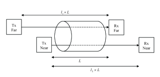
Figure 2: (2) Loop topology of the Near-Far problem in DSL. (2) Typical VDSL2 channel

TABLE II: DFDM implementation for the Near-Far scenario

1. Let $R_{d}$ = preassigned target rate for the near user.
2. Estimate the received noise PSD.
3. find $f_{c}$, the minimal $f$ such that the near user can achieve rate $R_{d}$ using frequencies above $f_{c}$.
4. Allocate the minimal amount of power needed for achieving $R_{d}$ using only frequencies grater than $f_{c}$.

VI Simulations

In this section we examine the rate region of the DFDM algorithm compared to FM-IWF. We have also simulated the OSM method [18], [19] which is a DSM level 2 in order to have an upper bound on the performance of DSM level 1 techniques. The channel transfer matrix is a measured binder provided by France Telecom research labs [22]. The simulations global parameters are VDSL 998 band plan up to 12 MHz, a maximum power constraint of $30mW$ (15 dBm) and a white noise PSD of $-140dBm/Hz$. In addition the frequency Division Duplex (FDD) 998 bandplan is used. We have simulate two scenarios:

• Central office / Remote Terminal Downstream.

• Upstream with non-identical locations.

The first scenario represent downstream setup where a central office (CO) with $8\times 3.6$ km ADSL lines is sharing a binder with a remote terminal (RT) with $8\times 0.9$ km VDSL lines. The RT is located 2.7 km from the CO as depicted in Figure 3. In the second simulation set we have studied upstream coordination. We have used two clusters of VDSL users sharing the same binder transmitting to the same RT. The far group contained 8 lines located 1.2 km from the RT while the near group contained 8 lines located just 600m from the RT, as depicted in Figure 3. Since in the VDSL 998 bandplan the lowest US frequency is 3.75 MHz the near far problem is much more pronounced than in ADSL.

Looking at the DS scenario. The achieved rate regions of the three methods are depicted in Figure 4. We can clearly see the advantage of the DFDM over the FM-IWF. The PSDs of the DFDM and the FM IWF methods corresponding to a 60 Mbps service on the RT lines are shown on Figure 4. For this value of $R_{d}$ there is no overlap between the frequencies used by each cluster of users resulting in no interference to CO users from RT users. This is the best case for the CO users since actually the near far problem has vanished and the achieved rate of the average CO user is the same as the RT was not transmitting at all. Figure 5 shows the received SINR of an average CO user for both methods. Its implies that for $R_{d}$ for which $f_{c}$ is grater than the maximal frequency used by the CO users the gain using DFDM has two factors. The first factor is that the DFDM’s SINR is grater or equal (since there is no interference from the RT) than the FM IWF one. The second is that the CO users available bandwidth is larger using DFDM than the FM IWF bandwidth. Both originate from the orthogonality of the transmission bands and both factors have positive contribute on the achieved rate of the CO users. Where $R_{d}$ is close to the RT maximal achievable rate $f_{c}$ is getting smaller and the available bandwidth for the CO is decreased. Figure 5 demonstrates this for $R_{d}=72$ Mbps. This design rate is almost $0.93\cdot R_{RT,max}$ and thus even by applying DFDM the RT PSD occupies most of the low frequencies regime. This causes the bandwidth of the CO users to decrease to 0.6 Mhz and in addition to a degradation in the SINR. As a consequence for this $R_{d}$ FM IWF achieves better rate for the CO users than DFDM. However as can be seen the difference is marginal.

Turning to the upstream scenario. Figure 6 depicts the rate region achieved by the different DSM methods. Not only the DFDM outperforms the FM IWF method in this scenario, the rate region obtained by the DFDM method is very close to the upper bound given by a fully coordinated spectrum management using the OSM algorithm. Moreover in this scenario the DFDM is better than or equal to the FM-IWF for all achievable rates of the strong user.

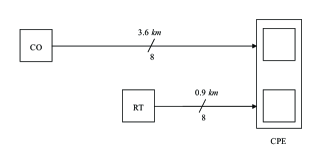
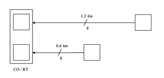
Figure 3: (3) CO/RT downstream setup. (3)Near-Far upstream setup

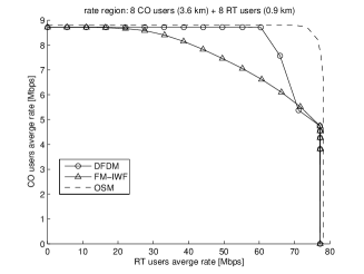
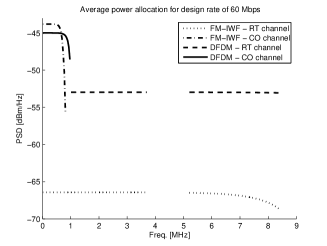
Figure 4: (4)Downstream - Rate region for 8 VDSL based RT and 8 ADSL based CO using FM-IWF and DFDM. (4) Downstream PSD for FM-IWF and DFDM.

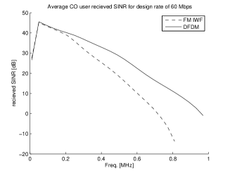
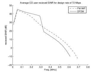
Figure 5: Average CO user received SINR for FM-IWF and DFDM for RT user at 60 Mbps (5 ) and 72 Mbps (5 ) .

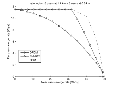
Figure 6: Upstream - Comparison of the rate region for 8 Far users and 8 Near users using FM-IWF and DFDM.

VII Conclusions

In this paper we have analyzed the iterative water filling algorithm for several simple channels using game theoretic techniques. We have shown that the IWF algorithm is subject to the prisoner’s dilemma by providing explicit characterization of its rate region for these cases. Based on these insights we proposed a distributed coordination algorithm improving the rate region in near-far scenarios. Finally we have provided experimental analysis of these two algorithms and the optimal centralized algorithm on measured channels.

VIII Appendix A: Proof of the existence of Nash equilibrium

In this section we prove that for every sequence of intervals $\{I_{1},\ldots,I_{k}\}$ ,the Gaussian interference game has a Nash equilibrium point. Our proof is based on the technique of [5], (see also [6]), adapted to the water-filling strategies in the game GI. While the result follows from standard game theoretic results, it is interesting to see the continuity of the water-filling strategy as the reason for the existence of the Nash equilibrium.

Theorem VIII.1

For any finite partition $\{I_{1},\ldots,I_{k}\}$ a Nash equilibrium in the Gaussian interference game $GI_{\{I_{1},\ldots,I_{k}\}}$ exists.

Proof: For each player $i$ define the water-filling function $W_{i}(\mbox{${\bf p}$}_{1},\ldots,\mbox{${\bf p}$}_{N}):\hbox{{\bf B}}{\rightarrow}\hbox{{\bf B}}_{i}$, which is the power distribution that maximizes $C^{i}$ given that for every $j\neq i$ player $j$ uses the power distribution $\mbox{${\bf p}$}_{j}$ subject to the power limitation $P_{i}$. The value of $W_{i}(\mbox{${\bf p}$}_{1},\ldots,\mbox{${\bf p}$}_{n})$ is given by water-filling with total power of $P_{i}$ against the noise power distribution composed of

$$N_{i}(k)=\frac{1}{|h_{i}(k)|^{2}}\left[\sum_{j\neq i}|h_{i}j(k)|^{2}p_{j}(k)+n_{i}(k)\right]$$ (59)

where for all $k$, $n_{i}(k)>0$ is the external noise power in the $k$’th band.

Claim VIII.1

$W_{i}(\mbox{${\bf x}$}_{1},\ldots,\mbox{${\bf x}$}_{N})$ is a continuous function.

Proof: We shall not prove this in detail. However informally this fact is very intuitive since small variations in the noise and interference power distributions will lead to small changes in the waterfilling response. The proof of theorem VIII.1 now easily follows from the Brauwer fixed point theorem. The function $\hbox{{\bf W}}=[W_{1},\ldots,W_{N}]$ maps B into itself. Since B is compact subset of a finite dimensional Euclidean space W has a fixed point $\left[\mbox{${\bf p}$}_{1},\ldots,\mbox{${\bf p}$}_{N}\right]^{T}$. This means that

$$\hbox{{\bf W}}(\left[\mbox{${\bf p}$}_{1},\ldots,\mbox{${\bf p}$}_{N}\right]^{T})=\left[\mbox{${\bf p}$}_{1},\ldots,\mbox{${\bf p}$}_{N}\right]^{T}$$

By the definition of W this means that each $\mbox{${\bf p}$}_{i}$ is the result of player $i$ water-filling its power against the interference generated by $\{\mbox{${\bf p}$}_{j}:j\neq i\}$ subject to its power constrain . Therefore $\left[\mbox{${\bf p}$}_{1},\ldots,\mbox{${\bf p}$}_{N}\right]^{T}$ is a Nash equilibrium for $GI_{\{I_{1},\ldots,I_{K}\}}$.

IX Appendix B: Bounds on the rate region of dynamic FDM

We can now obtain similar equations defining a dynamic FDM strategy, where the Bully uses the minimal fraction $\lambda W_{1}$ of the first band to achieve $R_{2}$. The main concept of this method is to minimize the interference to the weak user. This translates to minimize $\lambda$ for any given $R_{2}$. As a consequence we will not apply any power backoff (i.e. $\tau=1$) in order to maximize the power at the second band. The minimization of $\lambda$ is done through the maximization of the achieved rate for any given $\lambda$. Since the noise PSD is equal for both bands (recall that we neglect the interference from the weak user at the first band) maximizing the rate is equal to waterfill the power along a new single band channel with effective bandwidth of $\lambda W_{1}+W_{2}$ where $\lambda$ is chosen such the following equation holds

$$R_{2}=(\lambda W_{1}+W_{2})\log_{2}\left(1+\frac{P}{(\lambda W_{1}+W_{2})N_{2}}\right)$$ (60)

In order to get upper and lower bounds on $R_{1}$ under the new strategy we can bound the total used bandwidth

$$W_{2}\leq\lambda W_{1}+W_{2}\leq W_{1}+W_{2}$$ (61)

Thus we get

$$R_{2}\leq(\lambda W_{1}+W_{2})\log_{2}\left(1+\frac{P}{W_{2}N_{2}}\right)$$ (62)

and we derive that $\lambda\geq\lambda_{\min}$, where

$$\lambda_{\min}=\frac{\frac{R_{2}}{\log_{2}(1+\frac{SNR_{2}}{W_{2}})}-W_{2}}{W_{1}}$$ (63)

on the other hand

$$R_{2}\geq(\lambda W_{1}+W_{2})\log_{2}\left(1+\frac{P}{(W_{1}+W_{2})N_{2}}\right)$$ (64)

and similarly $\lambda\leq\lambda_{\max}$, where

$$\lambda_{\max}=\frac{\frac{R_{2}}{\log_{2}(1+\frac{SNR_{2}}{(W_{1}+W_{2})})}-W_{2}}{W_{1}}$$ (65)

Recall that $0\leq\lambda\leq 1$, if for given $R_{2}$ the obtained $\lambda$ is grater than 1 this implies that the given rate doesn’t lie in the achievable rate region of the bully. On the other hand a negative $\lambda$ implies that the bully can achieve the desired rate by the use of the second band solely (i.e. we will set $\lambda$ to zero).

The rate of user I is achieved by water-filling in the first band. This results in

$$R_{1}=(1-\lambda)W_{1}\log_{2}\left(1+\frac{\alpha P_{1,1-\lambda}}{(1-\lambda)W_{1}N_{1}}\right)+\lambda W_{1}\log_{2}\left(1+\frac{\alpha P_{1,\lambda}}{\lambda W_{1}N_{1}+\beta P_{1}}\right)$$ (66)

In order to evaluate this expression we first need to find $P_{1}$ which is user II power allocation at the band $\lambda W_{1}$. Moreover we need to compute $\{P_{1,1-\lambda},P_{1,\lambda}\}$ the power allocation vector of user I. $P_{1}$ is the power allocation at the first band of a two bands channel with equal noise PSD and with no power backoff. We have seen above that in this case we get $P_{1}=\tilde{\rho}P$ where $\tilde{\rho}=\frac{\lambda W_{1}}{\lambda W_{1}+W_{2}}$ hence

$$P_{1}=\frac{\lambda W_{1}}{\lambda W_{1}+W_{2}}P$$ (67)

$P_{1,1-\lambda}$ and $P_{1,\lambda}$ are the power allocation of user I along the two sub-bands at first band. Those parameters determined by WF where we define the power level in each sub-band as $\tilde{P}_{1,1-\lambda}$ and $\tilde{P}_{1,\lambda}$. Thus we have

$$\begin{array}[]{c}\tilde{P}_{1,1-\lambda}=\tilde{P}_{1,\lambda}+\frac{P_{1}}{\lambda W_{1}}\\ (1-\lambda)W_{1}\tilde{P}_{1,1-\lambda}+\lambda W_{1}\tilde{P}_{1,\lambda}=P\end{array}$$ (68)

The first equation in (68) stands for the constant level of power + noise at each sub-band while the second equation applies the total power constraint. solving (68) we get

$$\begin{array}[]{l}P_{1,1-\lambda}=(1-\lambda)W_{1}\tilde{P}_{1,1-\lambda}=P\left((1-\lambda)W_{1}+\lambda(1-\lambda)W_{1}^{2}\frac{1}{\lambda W_{1}+W_{2}}\right)\\ P_{1,\lambda}=\lambda W_{1}\tilde{P}_{1,\lambda}=P\left(\lambda W_{1}P-\lambda(1-\lambda)W_{1}^{2}\frac{1}{\lambda W_{1}+W_{2}}\right)\end{array}$$ (69)

substituting (69) and (67) in (66) we get

$$R_{1}=(1-\lambda)W_{1}\log_{2}\left(1+\frac{\alpha P\left(1+\lambda W_{1}\frac{1}{\lambda W_{1}+W_{2}}\right)}{N_{1}}\right)+\lambda W_{1}\log_{2}\left(1+\frac{\alpha P\left(1-(1-\lambda)W_{1}\frac{1}{\lambda W_{1}+W_{2}}\right)}{N_{1}+\beta\frac{P}{\lambda W_{1}+W_{2}}}\right)$$ (70)

Since the first sub-band (i.e. $(1-\lambda)W_{1}$) is interference free it is clear that $R_{1}$ is monotonically decreasing with $\lambda$. Hence we can derive upper and lower bounds on the achieved rate $R_{1}$ by substituting (63) and (65) respectively.

References

- [1] J.M. Cioffi ed. Dynamic spectrum management report (draft). ANSI Cont. NIPP-NAI-2005-0031R1, San Francisco, CA, April, 2003.
- [2] S. Chung, J. Lee, S. Kim, and J.M. Cioffi, “On the convergence of iterative waterfilling in the frequency selective gaussian interference channel,” Preprint, 2002.
- [3] S. Chung, S. Kim, and J. Cioffi, “On the existence and uniqueness of a Nash equilibrium in frequency selective gaussian interference channel,” Preprint, 2002.
- [4] S. Chung; Cioffi, J.M.; Rate and power control in a two-user multicarrier channel with no coordination: the optimal scheme versus a suboptimal method IEEE Transactions on Communications, Volume 51, Issue 11, Nov. 2003 Page(s):1768 - 1772
- [5] H. Nikaido and K. Isoida, “Note on non-cooperative convex games,” Pacific Journal of Matematics, vol. 5, pp. 807–815, 1955.
- [6] T. Basar and G. Olsder, Dynamic non-cooperative game theory. Academic Press, 1982.
- [7] G. Owen, Game theory, third edition. Academic Press, 1995.
- [8] W. Yu, G. Ginis, and J. Cioffi, “Distributed multiuser power control for digital subscriber lines,” IEEE Journal on Selected areas in Communications, vol. 20, pp. 1105–1115, june 2002.
- [9] G. Ginis and J.M. Cioffi. Vectored transmission for digital subscriber line systems. IEEE Journal on Selected Areas in Communications, 20(5):1085–1104, 2002.
- [10] T.M. Cover and J.A. Thomas. Elements of information theory. Wiley series in telecommunications, 1991.
- [11] W. Yu, G. Ginis and J.M. Cioffi. An adaptive multiuser power control algorithm for VDSL Global Telecommunications Conference, 2001. GLOBECOM ’01. IEEE Volume 1, 25-29 Nov. 2001 Page(s):394 - 398 vol.1
- [12] W. Yu and J.M. Cioffi Competitive equilibrium in the Gaussian interference channel. Proceedings. IEEE International Symposium on Information Theory, 2000. 25-30 June 2000 pp.431
- [13] K.B. Song, S. Chung, G. G. Ginis, and J. Cioffi. Dynamic spectrum management for next-generation DSL systems. IEEE Comm. Magazine, 40(10):101–109, 2002.
- [14] W. Yu and W. Rhee and S. Boyd and J.M. Cioffi. Iterative waterfilling for gaussian vector multiple-access channels. IEEE Transactions on Information Theory, vol. 50, no. 1, pp. 145-152, 200
- [15] Z.-Q. Luo and J.-S. Pang. Analysis of Iterative Waterfilling Algorithm for Multiuser Power Control in Digital Subscriber Lines. Submitted to the special issue of EURASIP Journal on Applied Signal Processing on Advanced Signal Processing Techniques for Digital Subscriber Lines.
- [16] M.M. Flood. Some experimenatal Games. Research Memorandum RM-789. Rand corporation. 1952
- [17] W. Poundstone Prisoner’s dilemma. Random House. 1992
- [18] R. Cendrillon, W. Yu, M. Moonen, J. Verlinden and T. Bostoen. Optimal multiuser spectrum management for digital subscriber lines. IEEE International Conference on Communications, 2004, vol. 1, pp. 1-5
- [19] R. Cendrillon, W. Yu, M. Moonen, J. Verliden, T. Bostoen. Optimal Multi-user Spectrum Management for Digital Subscriber Lines. To appear in IEEE Transactions on Communications 2005.
- [20] A. Laufer and A. Leshem. Distributed coordination of spectrum and the prisoner’s dilemma. To appear in IEEE workshop on dynamic spectrum access networks, DYSPAN 2005. Baltimore, MD. back-off: A simplified DSM algorithm for coexistence between RT and CO based deployments
- [21] A. Leshem. Dynamic FDM and Dynamic DS power back-off: A simplified DSM algorithm for coexistence between RT and CO based deployments. ANSI Cont. T1E1.4/2003-049. Costa Mesa, CA, March 2003.
- [22] E. Karipidis, N. sidiropoulos, A. Leshem, L. Youming, R. Tarafi and M. Ouzzif. Crosstalk models for short VDSL2 lines from measured 30 MHz Data. To be published in European Journal on applied signal processing.
- [23] J.M. Cioffi and M. Mosheni Band Preference in Water-filling with DSM. Contribution T1E1.4/2003-321R1. T1E1.4. San Diego, December 2003.