Conjunctive Queries over Trees

GEORG GOTTLOB
Oxford University
   Oxford    United Kingdom
CHRISTOPH KOCH
Universität des Saarlandes
   Saarbrücken    Germany
KLAUS U. SCHULZ
Ludwig-Maximilians-Universität München
   Munich    Germany
Abstract

We study the complexity and expressive power of conjunctive queries over unranked labeled trees represented using a variety of structure relations such as “child”, “descendant”, and “following” as well as unary relations for node labels. We establish a framework for characterizing structures representing trees for which conjunctive queries can be evaluated efficiently. Then we completely chart the tractability frontier of the problem and establish a dichotomy theorem for our axis relations, i.e., we find all subset-maximal sets of axes for which query evaluation is in polynomial time and show that for all other cases, query evaluation is NP-complete. All polynomial-time results are obtained immediately using the proof techniques from our framework. Finally, we study the expressiveness of conjunctive queries over trees and show that for each conjunctive query, there is an equivalent acyclic positive query (i.e., a set of acyclic conjunctive queries), but that in general this query is not of polynomial size.

category:
E.1 DATA STRUCTURES Trees
category:
F.1.3 COMPUTATION BY ABSTRACT DEVICES Complexity Classes – Reducibility and completeness
category:
F.2.2 ANALYSIS OF ALGORITHMS AND PROBLEM COMPLEXITY Nonnumerical Algorithms and Problems – Computations on discrete structures
category:
H.2.3 DATABASE MANAGEMENT Languages – Query languages
category:
H.2.4 DATABASE MANAGEMENT Systems – Query processing
category:
I.7.2 TEXT PROCESSING Document Preparation – Markup languages
keywords:
Complexity, Expressiveness, Succinctness, Conjunctive queries, Trees, XML
terms: Theory, Languages, Algorithms
{bottomstuff}

This work was partially supported by project No. Z29-N04 of the Austrian Science Fund (FWF), by a project of the German Research Foundation (DFG), and by the REWERSE Network of Excellence of the European Union.

An extended abstract [Gottlob et al. (2004)] of this work appeared in Proc.  23rd ACM SIGMOD-SIGACT-SIGART Symposium on Principles of Database Systems (PODS 2004), Paris, France, ACM Press, New York, USA, pp. 189 – 200.

Contact details: Georg Gottlob (Georg.Gottlob@comlab.ox.ac.uk), Oxford University Computing Laboratory, Wolfson Building, Parks Road, Oxford OX1 3QD, United Kingdom.

Christoph Koch (koch@infosys.uni-sb.de), Lehrstuhl für Informationssysteme, Universität des Saarlandes, D-66123 Saarbrücken, Germany.

Klaus U. Schulz (schulz@cis.uni-muenchen.de), Centrum für Informations- und Sprachverarbeitung, Ludwig-Maximilians-Universität München, D-80536 München, Germany.

1 Introduction

The theory of conjunctive queries over relational structures is, from a certain point of view, the greatest success story of the theory of database queries. These queries correspond to the most common queries in database practice, e.g.  SQL select-from-where queries with conditions combined using “and” only. Their evaluation problem has also been considered in different contexts and under different names, notably as the Constraint Satisfaction problem in AI [Kolaitis and Vardi (1998), Dechter (2003)] and the H-coloring problem in graph theory [Hell and Nesetril (2004)]. Conjunctive queries are surprisingly well-behaved: Many important properties hold for conjunctive queries but fail for more general query languages (cf.  [Chandra and Merlin (1977), Abiteboul et al. (1995), Maier (1983)]).

Unranked labeled trees are a clean abstraction of HTML, XML, LDAP, and linguistic parse trees. This motivates the study of conjunctive queries over trees, where the tree structures are represented using unary node label relations and binary relations (often referred to as axes) such as Child, Descendant, and Following.

XML Queries. Conjunctive queries over trees are naturally related to the problem of evaluating queries (e.g., XQuery or XSLT) on XML data (cf.  [Deutsch and Tannen (2003a)]). However, conjunctive queries are a cleaner and simpler model whose complexity and expressiveness can be formally studied (while XQuery and XSLT are Turing-complete).

(Acyclic) conjunctive queries over trees are a generalization of the most frequently used fragment of XPath. For example, the XPath query //A[B]/following::C is equivalent to the (acyclic) conjunctive query

$$Q(z)\leftarrow\textit{A}(x),\;\textit{Child}(x,y),\;B(y),\;\textit{Following}(x,z),\;C(z).$$

While XPath has been studied extensively (see e.g. [Gottlob et al. (2005), Gottlob et al. (2005)] on its complexity, [Benedikt et al. (2003), Olteanu et al. (2002)] on its expressive power, and [Hidders (2003)] on the satisfiability problem), little work so far has addressed the theoretical properties of cyclic conjunctive queries over trees. Sporadic results on their complexity can be found in [Meuss et al. (2001), Gottlob and Koch (2002), Gottlob and Koch (2004), Meuss and Schulz (2001)].

Data extraction and integration. (Cyclic) conjunctive queries on trees have been used previously in data integration, where queries in languages such as XQuery were canonically mapped to conjunctive queries over trees to build upon the existing work on data integration with conjunctive queries [Deutsch and Tannen (2003a), Deutsch and Tannen (2003b)]. Another application is Web information extraction using a datalog-like language over trees [Baumgartner et al. (2001), Gottlob and Koch (2004)]. (Of course, each nonrecursive datalog rule is a conjunctive query.)

Queries in computational linguistics. A further area in which such queries are employed is computational linguistics, where one needs to search in, or check properties of, large corpora of parsed natural language. Corpora such as Penn Treebank [LDC (1999)] are unranked trees labeled with the phrase structure of parsed (for Treebank, financial news) text. A query asking for prepositional phrases following noun phrases in the same sentence can be phrased as the conjunctive query

$$Q(z)\leftarrow S(x),\;\textit{Descendant}(x,y),\;\textit{NP}(y),\;\textit{Descendant}(x,z),\;\textit{PP}(z),\;\textit{Following}(y,z).$$
\drawline(525,720)(75,270) \blacken\drawline(117.426,333.640)(75.000,270.000)(138.640,312.426)(117.426,333.640) \drawline(525,720)(975,270) \blacken\drawline(911.360,312.426)(975.000,270.000)(932.574,333.640)(911.360,312.426) \drawline(75,270)(975,270) \blacken\drawline(900.000,255.000)(975.000,270.000)(900.000,285.000)(900.000,255.000) $S$DescendantDescendant$PP$ $NP$Following
Figure 1: A query graph.

Figure 1 shows this query in the intuitive graphical notation that we will use throughout the article (in which nodes correspond to variables, node labels to unary atoms, and edges to binary atoms).

Dominance constraints. Another important issue in computational linguistics are conjunctions of dominance constraints [Marcus et al. (1983)], which turn out to be equivalent to (Boolean) conjunctive queries over trees. Dominance constraints have been influential as a means of incompletely specifying parse trees of natural language, in cases where (intermediate) results of parsing and disambiguation remain ambiguous. One problem of practical importance is the rewriting of sets of dominance constraints into equivalent but simpler sets (in particular, so-called solved forms [Bodirsky et al. (2004)], which correspond to acyclic queries). This implies that studying the expressive power of conjunctive queries over trees, and the problem of deciding whether there is a set of acyclic conjunctive queries equivalent to a given conjunctive query, is relevant to computational linguistics.

Higher-order unification. The query evaluation problem for conjunctive queries over trees is also closely related to the context matching problem111To be precise, the analogy is most direct with ranked trees., a variant of the well-known context-unification problem [Schmidt-Schauß and Schulz (1998), Schmidt-Schauß and Schulz (2002)]. Some tractability frontier for the context matching problem is outlined in [Schmidt-Schauß and Stuber (2001)]. However, little insight is gained from this for the database context, since the classes studied in [Schmidt-Schauß and Stuber (2001)] become unnatural when formulated as conjunctive queries222These conjunctive queries require node inequality $\neq$ as a binary relation in addition to the tree structure relations. If $\neq$ is removed, the queries become acyclic. However, it is easy to see that already conjunctive queries using only the inequality relation over a fixed tree of three nodes are NP-complete, by a reduction from Graph 3-Colorability..

Contributions

Given the substantial number of applications that we have hinted at above and the nice connection between database theory, computational linguistics, and term rewriting, it is surprising that conjunctive queries over trees have never been the object of a concerted study333Of course, as mentioned above, there are a number of papers that implicitly contain relevant results [Meuss et al. (2001), Meuss and Schulz (2001), Hidders (2003), Schmidt-Schauß and Stuber (2001)]. The papers [Hell et al. (1996a), Hell et al. (1996b)] address the complexity of a notion of tree homomorphisms that is uncomparable to the one used in database theory, and the results there are orthogonal..

In particular, three questions seem worth studying:

  1. 1.

    The complexity of (cyclic) conjunctive queries on trees has only been scratched in the literature. There is little understanding of how the complexity of conjunctive queries over trees depends on the relations used to model the tree.

  2. 2.

    There is a natural connection between conjunctive queries and XPath. Since all XPath queries are acyclic, the question arises whether the acyclic positive queries (i.e., unions of acyclic conjunctive queries) are as expressive as the full class of conjunctive queries over trees.444This is equivalent to asking whether for all conjunctive queries over trees there exist equivalent positive Core XPath queries [Gottlob et al. (2005)].

  3. 3.

    If that is the case, how much bigger do the acyclic versions of queries get than their cyclic counterparts? Except from being of theoretical interest, first translating queries into their acyclic versions, if that is possible, and then evaluating them as such may be a practical query evaluation strategy, because there are particularly good algorithms for evaluating such queries [Yannakakis (1981), Chekuri and Rajaraman (1997), Flum et al. (2002), Gottlob and Koch (2004)].

We thus study conjunctive queries on tree structures represented using the XPath axis relations child, descendant, descendant-or-self, following-sibling, and following. Since we are free to use these relations with any pair of variables of our conjunctive queries (differently from XPath), these five axes render all others, i.e.  parent, ancestor, ancestor-or-self, preceding-sibling, and preceding, redundant. Typed child axes such as attribute are redundant with the child axis and unary relations in our framework.

For a more elegant framework, we study the axes Child, $\textit{Child}^{*}$ (= descendant-or-self), $\textit{Child}^{+}$ (= descendant), NextSibling, $\textit{NextSibling}^{*}$, $\textit{NextSibling}^{+}$ (= following-sibling), and Following. (NextSibling and $\textit{NextSibling}^{*}$ are not supported in XPath but are nevertheless considered here.) Subsequently, we denote this set of all axes considered in this article by ${\bf Ax}$.

The main contributions of this article are as follows.

  • In [Gutjahr et al. (1992)] it was shown that the $H$-coloring problem (cf. [Hell and Nesetril (2004)]), and thus Boolean conjunctive query evaluation, on directed graphs $H$ that have the so-called $\underline{X}$-property (pronounced “X-underbar-property”) is polynomial-time solvable. We determine which of our axis relations have the $\underline{X}$-property with respect to which orders of the domain elements. We show that the subset-maximal sets of axis relations for which the $\underline{X}$-property yields tractable query evaluation are the three disjoint sets

    $$\{\textit{Child},\textit{NextSibling},\textit{NextSibling}^{*},\textit{NextSibling}^{+}\},$$
    $$\{\textit{Child}^{*},\textit{Child}^{+}\},\quad\mbox{and}\quad\{\textit{Following}\}.$$
  • We prove that the conjunctive query evaluation problem for queries involving any two axes that do not have the $\underline{X}$-property with respect to the same ordering of the tree nodes is NP-complete.

    Thus the $\underline{X}$-property yields a complete characterization of the tractability frontier of the problem (under the assumption that P $\neq$ NP).

    Theorem 1.1

    Unless P = NP, for any $F\subseteq{\bf Ax}$, the conjunctive queries over structures with unary relations and binary relations from $F$ are in P if and only if there is a total order $<$ such that all binary relations in $F$ have the $\underline{X}$-property w.r.t. $<$.

    Moreover we have the dichotomy that for any of our tree structures, the conjunctive query evaluation problem is either in P or NP-complete.

    Child $\textit{Child}^{+}$ $\textit{Child}^{*}$ NextSibling $\textit{NextSibling}^{+}$ $\textit{NextSibling}^{*}$ Following
    Child in P NP-hard NP-hard in P in P in P NP-hard
    (4.5) (5.1) (5.1) (4.5) (4.5) (4.5) (5.3)
    $\textit{Child}^{+}$ in P in P NP-hard NP-hard NP-hard NP-hard
    (4.3) (4.3) (5.12) (5.12) (5.12) (5.5)
    $\textit{Child}^{*}$ in P NP-hard NP-hard NP-hard NP-hard
    (4.3) (5.8) (5.7) (5.10) (5.5)
    NextSibling in P in P in P NP-hard
    (4.5) (4.5) (4.5) (5.14)
    $\textit{NextSibling}^{+}$ in P in P NP-hard
    (4.5) (4.5) (5.14)
    $\textit{NextSibling}^{*}$ in P NP-hard
    (4.5) (5.14)
    Following in P
    (4.4)
    Table 1: Complexity results for signatures with one or two axes, with pointers to relevant theorems.

    Table 1 shows the complexities of conjunctive queries over structures containing unary relations and either one or two axes.555It was shown in [Gottlob and Koch (2004)] that conjunctive queries over Child and NextSibling are in P. Proposition 4.3 is from [Gottlob and Koch (2002)].) The other results are new.

    All NP-hardness results hold already for fixed data trees (query complexity [Vardi (1982)]). The polynomial-time upper bounds are established under the assumption that both data and query are variable (combined complexity).

  • We study the expressive power of conjunctive queries on trees. We show that for each conjunctive query over trees, there is an equivalent acyclic positive query (APQ) over the same tree relations. The blowup in size of the APQs produced is exponential in the worst case.

    It follows that there is an equivalent XPath query for each conjunctive query over trees, since each APQ can be translated into XPath (even in linear time).

  • Finally, we provide a result that sheds some light at the succinctness of (cyclic) conjunctive queries and which demonstrates that the blow-up observed in our translation is actually necessary. We prove that there are conjunctive queries over trees for which no equivalent polynomially-sized APQ exists.

The structure of the article is as follows. We start with basic notions in Section 2. Section 3 introduces the $\underline{X}$-property and the associated framework for finding classes of conjunctive queries that can be evaluated in polynomial time. Section 4 contains our polynomial-time complexity results. Section 5 completes our tractability frontier with the NP-hardness results. In Section 6, we provide our expressiveness results. Finally, we present our succinctness result in Section 7.

2 Preliminaries

Let $\Sigma$ be a labeling alphabet. Throughout the article, if not explicitly stated otherwise, we will not assume $\Sigma$ to be fixed. An unranked tree is a tree in which each node may have an unbounded number of children. We allow for tree nodes to be labeled with multiple labels. However, throughout the article, our tractability results will support multiple labels while our NP-hardness and expressiveness results will not make use of them.

We represent trees as relational structures using unary label relations $(\textit{Label}_{a})_{a\in\Sigma}$ and binary relations called axes. For a relational structure ${\cal A}$, let $A=|{\cal A}|$ denote the finite domain (in the case of a tree, the nodes) and let $||{\cal A}||$ denote the size of the structure under any reasonable encoding scheme (see e.g. [Ebbinghaus and Flum (1999)]). We use the binary axis relations Child (defined in the normal way) and NextSibling (where $\textit{NextSibling}(v,w)$ if and only if $w$ is the right neighboring sibling of $v$ in the tree), their transitive and reflexive and transitive closures (denoted $\textit{Child}^{+}$, $\textit{NextSibling}^{+}$, $\textit{Child}^{*}$, $\textit{NextSibling}^{*}$), and the axis Following, defined as

$$\textit{Following}(x,y)=\exists z_{1}\exists z_{2}\;\textit{Child}^{*}(z_{1},x)\land\textit{NextSibling}^{+}(z_{1},z_{2})\land\textit{Child}^{*}(z_{2},y).$$ (1)

This set of axes covers the standard XPath axes (cf. [World Wide Web Consortium (1999)]) by the equivalences $\textit{Child}^{+}=\textit{Descendant}$, $\textit{Child}^{*}=\textit{Descendant-or-self}$, and $\textit{NextSibling}^{+}=\textit{Following-sibling}$.

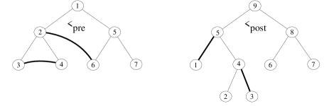
We consider three well-known total orderings on finite ordered trees. The pre-order $\leq_{pre}$ corresponds to a depth-first left-to-right traversal of a tree. If XML-documents are represented as trees in the usual way, the pre-order coincides with the document order. It is given by the sequence of opening tags of the XML elements (corresponding to nodes). The post-order $\leq_{post}$ corresponds to a bottom-up left-to-right traversal of the tree and is given by the sequence of closing tags of elements. Furthermore, we also consider the ordering $\leq_{bflr}$ which is given by the sequence of opening tags if we traverse the tree breadth-first left-to-right.

The $k$-ary conjunctive queries can be defined by positive existential first-order formulas without disjunction and with $k$ free variables. We will usually use the standard (datalog) rule notation for conjunctive queries (cf. [Abiteboul et al. (1995)]).

We call the 0-ary queries Boolean and the unary queries monadic. The containment of queries $Q$ and $Q^{\prime}$ is defined in the normal way: Query $Q$ is said to be contained in $Q^{\prime}$ (denoted $Q\subseteq Q^{\prime}$) iff, for all tree structures ${\cal A}$, $Q^{\prime}$ returns at least all tuples on ${\cal A}$ that $Q$ returns on ${\cal A}$. (To cover Boolean queries, tuples here may be nullary.) Two queries $Q,Q^{\prime}$ are called equivalent iff $Q\subseteq Q^{\prime}$ and $Q^{\prime}\subseteq Q$.

Let $Q$ be a conjunctive query and let $\textit{Var}(Q)$ denote the variables appearing in $Q$. The query graph of $Q$ over unary and binary relations is the directed multigraph $G=(V,E)$ with edge labels and multiple node labels such that $V=\textit{Var}(Q)$, node $x$ is labeled $P$ iff $Q$ contains unary atom $P(x)$, and $E$ contains labeled directed edge $x\stackrel{{\scriptstyle R}}{{\rightarrow}}y$ if and only if $Q$ contains binary atom $R(x,y)$. Figure 1 shows an example of such a query graph. Our notion of query graph is sometimes called positive atomic diagram in model theory or the graph of the canonical database of a query in the database theory literature.

Throughout the article, we use lower case node and variable names and upper case label and relation names.

3 The X-Property

Let $Q$ be a conjunctive query and let $A$ denote the finite domain, i.e. in case of a tree the set of nodes. A pre-valuation for $Q$ is a total function $\Theta:\textit{Var}(Q)\rightarrow 2^{A}$ that assigns to each variable of $Q$ a nonempty subset of $A$. A valuation for $Q$ is a total function $\theta:\textit{Var}(Q)\rightarrow A$.

Let ${\cal A}$ be a relational structure of unary and binary relations. A pre-valuation $\Theta$ is called arc-consistent666This notion is well-known in constraint satisfaction, cf. [Dechter (2003)]. iff for each unary atom $P(x)$ in $Q$ and each $v\in\Theta(x)$, $P(v)$ is true (in ${\cal A}$) and for each binary atom $R(x,y)$ in $Q$, for each $v\in\Theta(x)$ there exists $w\in\Theta(y)$ such that $R(v,w)$ is true and for each $w\in\Theta(y)$ there exists $v\in\Theta(x)$ such that $R(v,w)$ is true.

Proposition 3.1 ((Folklore))

There is an algorithm which checks in time $O(||{\cal A}||\cdot|Q|)$ whether an arc-consistent pre-valuation of $Q$ on ${\cal A}$ exists, and if it does, returns one.

Proof 3.2.

We phrase the problem of computing $\Theta$ by deciding, for each $x,v$, whether $v\not\in\Theta(x)$ as an instance ${\cal P}$ of propositional Horn-SAT. The propositional predicates are the atoms (where $x\in\mathit{Vars}(Q)$, $v\in A$ are constants), and the Horn clauses are

$\{$ $\cup$
$\{$ $\cup$
$\{$

Let be the binary relation defined by ${\cal P}$ and let

$$T=(\mathit{Vars}(Q)\times A)-$$

be the complement of that relation. If there is a variable $x$ such that for no node $v$, $(x,v)\in T$, no arc-consistent pre-valuation of $Q$ on ${\cal A}$ exists and $Q$ is not satisfied. Otherwise, the pre-valuation defined by

$$\Theta(x)\mapsto\{v\mid(x,v)\in T\},$$

for each $x$, is obviously arc-consistent and contains all arc-consistent pre-valuations of $Q$ and ${\cal A}$.

Program ${\cal P}$ can be computed and solved (e.g. using Minoux’ algorithm [Minoux (1988)]), and the solution complemented, in time linear in the size of the program, which is $O(||{\cal A}||\cdot|Q|)$.

Actually, this algorithm computes the unique subset-maximal arc-consistent pre-valuation of $Q$ on ${\cal A}$.

A valuation $\theta$ is called consistent if it satisfies the query. In this case, for a Boolean query, we also say that the structure is a model of the query and the valuation a satisfaction. Obviously, a valuation is consistent if and only if the pre-valuation $\Theta$ defined by $\Theta(x)\mapsto\{\theta(x)\}$ is arc-consistent. Let $<$ be a total order on $A=|{\cal A}|$ and $\Theta$ be a pre-valuation. Then the valuation $\theta$ with $\theta(x)\mapsto v$ iff $v$ is the smallest node in $\Theta(x)$ w.r.t.  $<$ is called the minimum valuation w.r.t. $<$ in $\Theta$.

Definition 3.3.

Let ${\cal A}$ be a relational structure, $R$ a binary relation in ${\cal A}$, and $<$ a total order on $A=|{\cal A}|$. Then, $R$ is said to have the $\underline{X}$-property w.r.t. $<$ iff for all $n_{0},n_{1},n_{2},n_{3}\in A$ such that $n_{0}<n_{1}$ and $n_{2}<n_{3}$,

$$R(n_{1},n_{2})\land R(n_{0},n_{3})\Rightarrow R(n_{0},n_{2}).$$
\blacken\ellipse4848\ellipse4848\blacken\ellipse4848\ellipse4848\blacken\ellipse4848\ellipse4848\blacken\ellipse4848\ellipse4848\blacken\ellipse4848\ellipse4848\blacken\ellipse4848\ellipse4848\blacken\ellipse4848\ellipse4848\blacken\ellipse4848\ellipse4848\blacken\ellipse4848\ellipse4848\blacken\ellipse4848\ellipse4848\blacken\ellipse4848\ellipse4848\blacken\ellipse4848\ellipse4848\blacken\ellipse4848\ellipse4848\blacken\ellipse4848\ellipse4848\blacken\ellipse4848\ellipse4848\blacken\ellipse4848\ellipse4848\blacken\ellipse4848\ellipse4848\blacken\ellipse4848\ellipse48482177,1470)2177,345) 2177,345)2927,795) \blacken2870.405,743.550)2927.000,795.000)(2854.971,769.275)(2870.405,743.550) 2177,345)2927,570) \blacken2859.473,534.082)2927.000,570.000)(2850.853,562.816)(2859.473,534.082) 2927,1470)2927,345) 602,1320)602,870) \blacken587.000,945.000)602.000,870.000)(617.000,945.000)(587.000,945.000) \blacken194.426,933.640)152.000,870.000)(215.640,912.426)(194.426,933.640) 152,870)602,1320) 602,1320)1052,870) \blacken988.360,912.426)1052.000,870.000)(1009.574,933.640)(988.360,912.426) 2177,345)2927,1020) \blacken2881.287,958.678)2927.000,1020.000)(2861.218,980.977)(2881.287,958.678) 2177,345)2927,1245) \blacken2890.509,1177.781)2927.000,1245.000)(2867.463,1196.986)(2890.509,1177.781) 2177,795)2927,1020) \blacken2859.473,984.082)2927.000,1020.000)(2850.853,1012.816)(2859.473,984.082) 2177,345)2927,1470) \blacken2897.878,1399.276)2927.000,1470.000)(2872.917,1415.917)(2897.878,1399.276) 2177,795)2927,1245) \blacken2870.405,1193.550)2927.000,1245.000)(2854.971,1219.275)(2870.405,1193.550) 602,870)827,420) \blacken780.043,480.374)827.000,420.000)(806.875,493.790)(780.043,480.374) 602,870)377,420) \blacken397.125,493.790)377.000,420.000)(423.957,480.374)(397.125,493.790) 602,1320)827,420) \blacken794.258,489.123)827.000,420.000)(823.362,496.399)(794.258,489.123) 602,1320)377,420) \blacken380.638,496.399)377.000,420.000)(409.742,489.123)(380.638,496.399) 123456123564124563(b)(a)
Figure 2: The $\underline{X}$-property. Graph (a) and its illustration by arcs between two bars (b). For crossing arcs $R(u,v)$ and $R(u^{\prime},v^{\prime})$, say $u<u^{\prime}$ and $v^{\prime}<v$, there must be an arc $R(u,v^{\prime})$.

Figure 2 illustrates why the property is called $\underline{X}$ (read as “X-underbar”). Let us consider two vertical bars both representing the order $<$ bottom-up (i.e., with the smallest value at the bottom). Let each edge $(u,v)$ in $R$ be represented by an arc from node $u$ on the left bar to node $v$ on the right bar. Then, whenever there are two crossing arcs $(u,v)$ and $(u^{\prime},v^{\prime})$ in this diagram, then there must be an arc $(\mbox{min}(u,u^{\prime}),\mbox{min}(v,v^{\prime}))$, the “underbar”, in the diagram as well.

Remark 3.4.

The $\underline{X}$-property777In [Gottlob et al. (2004)], this property was called hemichordality. was introduced in [Gutjahr et al. (1992)], where it was shown that the $H$-coloring problem (or equivalently the conjunctive query evaluation problem) on graphs $H$ with the $\underline{X}$-property is polynomial-time solvable (see also [Hell and Nesetril (2004)]). In the remainder of this section, we rephrase this result as a tool for efficiently evaluating conjunctive queries.

Let ${\cal A}$ be a structure of unary and binary relations and let $<$ be a total order on $|{\cal A}|$. Structure ${\cal A}$ is said to have the $\underline{X}$-property w.r.t. $<$ if all binary relations $R$ in ${\cal A}$ have the $\underline{X}$-property w.r.t. $<$.

Lemma 3.5.

Let ${\cal A}$ be a structure with the $\underline{X}$-property w.r.t. $<$ and let $\Theta$ be an arc-consistent pre-valuation on ${\cal A}$ for a given conjunctive query over the relations of ${\cal A}$. Then, the minimum valuation in $\Theta$ w.r.t. $<$ is consistent.

Proof 3.6.

Let $\theta$ denote the minimum valuation in $\Theta$ w.r.t. $<$. To prove $\theta$ consistent, we only need to show the following: If $R(x,y)$ is any binary atom of $Q$ with variables $x,y$ then $R(x,y)$ holds under assignment $\theta$, i.e. $R(\theta(x),\theta(y))$ is true in ${\cal A}$.

Let $\theta(x)=n_{0}$ and $\theta(y)=n_{2}$. Since $\Theta$ is arc-consistent there exists a node $n_{1}\in\Theta(x)$ such that $R(n_{1},n_{2})$ and a node $n_{3}\in\Theta(y)$ such that $R(n_{0},n_{3})$. If $n_{0}=n_{1}$ or $n_{2}=n_{3}$ then $R(\theta(x),\theta(y))=R(n_{0},n_{2})$ is true and we are done. Otherwise, since $\theta$ is a minimum valuation we have $n_{0}<n_{1}$ (because $n_{0}=\theta(x)=\min\Theta(x)$, $n_{1}\in\Theta(x)$, and $n_{0}\neq n_{1}$) and $n_{2}<n_{3}$ (because $n_{2}=\theta(y)=\min\Theta(y)$, $n_{3}\in\Theta(y)$, and $n_{2}\neq n_{3}$). Then it follows from Definition 3.3 that $R(n_{0},n_{2})$.

Clearly, if no arc-consistent pre-valuation of $Q$ on ${\cal A}$ exists, there is no consistent valuation for $Q$ on ${\cal A}$.

Theorem 3.7.

Given a structure ${\cal A}$ with the $\underline{X}$-property w.r.t. $<$ and a Boolean conjunctive query $Q$ over ${\cal A}$, $Q$ can be evaluated on ${\cal A}$ in time $O(||{\cal A}||\cdot|Q|)$.

Proof 3.8.

By Lemma 3.5, all we need to do to check whether a Boolean query $Q$ is satisfied is to try to compute the subset-maximal arc-consistent pre-valuation $\Theta$ with respect to $Q$. By Proposition 3.1, this can be done in time $O(||{\cal A}||\cdot|Q|)$. If it exists, $Q$ returns true; otherwise, $Q$ returns false.

If follows that checking whether a given tuple ${\langle a_{1},\dots,a_{k}\rangle}$ is in the result of a $k$-ary conjunctive query on structures with the $\underline{X}$-property w.r.t. some order can be decided in time $O(||{\cal A}||\cdot|Q|)$ as well. All we need to do is to add (new) singleton unary relations $X_{1}=\{a_{1}\},\dots,X_{k}=\{a_{k}\}$ to ${\cal A}$ and to rewrite the query $Q(x_{1},\dots,x_{k})\leftarrow\Phi(x_{1},\dots,x_{k})$ into the Boolean query $Q\leftarrow\Phi(x_{1},\dots,x_{k})\land X_{1}(x_{1})\land\dots\land X_{k}(x_{k}).$ A $k$-ary conjunctive query $Q$ over ${\cal A}$ with $A=|{\cal A}|$ can thus be evaluated on ${\cal A}$ in time $O(|A|^{k}\cdot||{\cal A}||\cdot|Q|)$.

For relations that are subsets of the given total order $\leq$ (the reflexive closure of $<$), a slightly stronger condition for the $\underline{X}$-property w.r.t. $<$ can be given.

Lemma 3.9.

Let ${\cal A}$ be a structure, $<$ a total order on $A=|{\cal A}|$, and $R$ a binary relation of ${\cal A}$ such that $R\subseteq\leq$. Then, $R$ has the $\underline{X}$-property w.r.t. $<$ iff for all $n_{0},n_{1},n_{2},n_{3}\in A$ such that $n_{0}<n_{1}\leq n_{2}<n_{3}$,

$$R(n_{1},n_{2})\land R(n_{0},n_{3})\Rightarrow R(n_{0},n_{2}).$$
Proof 3.10.

Obviously, if $R$ has the $\underline{X}$-property w.r.t. $<$, then the condition of Definition 3.3 implies that the condition of our lemma holds. Conversely, since for all $n_{1},n_{2}$, $R(n_{1},n_{2})\Rightarrow n_{1}\leq n_{2}$, by our lemma, for all $n_{0},n_{1},n_{2},n_{3}\in A$ such that $n_{0}<n_{1}$ and $n_{2}<n_{3}$, $R(n_{1},n_{2})\land R(n_{0},n_{3})\Rightarrow R(n_{0},n_{2})$.

A symmetric version of Lemma 3.5 holds for relations $R\subseteq\geq$.

Lemma 3.11.

Let ${\cal A}$ be a structure, $<$ a total order on $A=|{\cal A}|$, and $R$ a binary relation of ${\cal A}$ such that $R\subseteq\geq$. Then, $R$ has the $\underline{X}$-property w.r.t. $<$ iff for all $n_{0},n_{1},n_{2},n_{3}\in A$ such that $n_{0}<n_{1}\leq n_{2}<n_{3}$,

$$R(n_{2},n_{1})\land R(n_{3},n_{0})\Rightarrow R(n_{2},n_{0}).$$
Proof 3.12.

Let $R^{\prime}=R^{-1}$. By Lemma 3.9, $R^{\prime}$ has the $\underline{X}$-property w.r.t. $<$ precisely if for all $n_{0},n_{1},n_{2},n_{3}\in A$, $n_{0}<n_{1}\leq n_{2}<n_{3}\land R^{\prime}(n_{1},n_{2})\land R^{\prime}(n_{0},n_{3})\Rightarrow R^{\prime}(n_{0},n_{2})$. Thus, $R$ has the $\underline{X}$-property w.r.t. $<$ iff the condition of our lemma holds.

4 Polynomial-Time Results

The results of Section 3 provide us with a simple technique for proving polynomial-time complexity results for conjunctive queries over trees. Indeed, there is a wealth of inclusions of axis relations in the total orders introduced in Section 2:

  1. 1.

    all the axes in ${\bf Ax}$ are subsets of the pre-order ${\leq_{\textit{\footnotesize pre}}}$,

  2. 2.

    $\textit{Child}^{-1}$, $(\textit{Child}^{+})^{-1}$, $(\textit{Child}^{*})^{-1}$, Following, NextSibling, $\textit{NextSibling}^{+}$, and $\textit{NextSibling}^{*}$ are subsets of the post-order ${\leq_{\textit{\footnotesize post}}}$, and

  3. 3.

    Child, $\textit{Child}^{+}$, $\textit{Child}^{*}$, NextSibling, $\textit{NextSibling}^{+}$, and $\textit{NextSibling}^{*}$ are subsets of the order ${\leq_{\textit{\footnotesize bflr}}}$.

Using Lemma 3.9, it is straightforward to show that

Theorem 4.1.

The axes

  1. 1.

    $\textit{Child}^{+}$ and $\textit{Child}^{*}$ have the $\underline{X}$-property w.r.t. ${<_{\textit{\footnotesize pre}}}$,

  2. 2.

    Following has the $\underline{X}$-property w.r.t. ${<_{\textit{\footnotesize post}}}$, and

  3. 3.

    Child, NextSibling, $\textit{NextSibling}^{*}$, and $\textit{NextSibling}^{+}$ have the $\underline{X}$-property w.r.t. $<_{\textit{\footnotesize bflr}}$.

Proof 4.2.

All proof arguments use Lemma 3.9.

We first show that $\textit{Child}^{*}$ has the $\underline{X}$-property w.r.t. ${<_{\textit{\footnotesize pre}}}$. (The proof for $\textit{Child}^{+}$ is similar.) Consider the nodes $n_{0},\dots,n_{3}$ such that $n_{0}\,{<_{\textit{\footnotesize pre}}}\,n_{1}\,{\leq_{\textit{\footnotesize pre}}}\,n_{2}\,{<_{\textit{\footnotesize pre}}}\,n_{3}$, $\textit{Child}^{*}(n_{0},n_{3})$, and $\textit{Child}^{*}(n_{1},n_{2})$. It is simple to see that ${\leq_{\textit{\footnotesize pre}}}$ is the disjoint union of $\textit{Child}^{*}$ and Following. Therefore, either $\textit{Child}^{*}(n_{0},n_{1})$, which implies $\textit{Child}^{*}(n_{0},n_{2})$, or $\textit{Following}(n_{0},n_{1})$. The latter case would yield $n_{3}{<_{\textit{\footnotesize pre}}}n_{1}$, a contradiction.

Next, we show that Following has the $\underline{X}$-property w.r.t. ${<_{\textit{\footnotesize post}}}$. Assume that

$$n_{0}\,{<_{\textit{\footnotesize post}}}\,n_{1}\,{\leq_{\textit{\footnotesize post}}}\,n_{2}\,{<_{\textit{\footnotesize post}}}\,n_{3}$$

and $\textit{Following}(n_{1},n_{2})$, $\textit{Following}(n_{0},n_{3})$. Clearly, the relation ${\leq_{\textit{\footnotesize post}}}$ is the disjoint union of Following and the inverse of $\textit{Child}^{*}$. Since $n_{0}{<_{\textit{\footnotesize post}}}n_{1}$ is true, either $\textit{Child}^{*}(n_{1},n_{0})$ or $\textit{Following}(n_{0},n_{1})$ must hold. In both cases it follows that $\textit{Following}(n_{0},n_{2})$. Thus, Following has the $\underline{X}$-property w.r.t. ${<_{\textit{\footnotesize post}}}$.

The fact that Child has the $\underline{X}$-property w.r.t. $<_{\textit{\footnotesize bflr}}$ follows vacuously from the characterization of Lemma 3.9: Assume that $n_{0}<_{\textit{\footnotesize bflr}}n_{1}\leq_{\textit{\footnotesize bflr}}n_{2}<_{\textit{\footnotesize bflr}}n_{3}$ and that $\textit{Child}(n_{1},n_{2})$ (thus $n_{0}<_{\textit{\footnotesize bflr}}n_{1}<_{\textit{\footnotesize bflr}}n_{2}<_{\textit{\footnotesize bflr}}n_{3}$) and $\textit{Child}(n_{0},n_{3})$. Because of $\textit{Child}(n_{0},n_{3})$, the node $n_{1}$ is at most one level below $n_{0}$ in the tree. There are two cases, (1) $\textit{Following}(n_{0},n_{1})$ and $n_{0}$, $n_{1}$ are on the same level in the tree or (2) $\textit{Following}(n_{1},n_{3})$ and $n_{1}$, $n_{3}$ are on the same level in the tree. In case (1), since $n_{3}$ is a child of $n_{0}$ and $n_{2}$ is a child of $n_{1}$, $n_{3}<_{\textit{\footnotesize bflr}}n_{2}$, contradiction. In case (2), since $n_{2}$ is a child of $n_{1}$, $n_{2}$ is one level below $n_{3}$ in the tree and thus $n_{3}<_{\textit{\footnotesize bflr}}n_{2}$, contradiction.

It is easy to verify that NextSibling, $\textit{NextSibling}^{*}$, and $\textit{NextSibling}^{+}$ have the $\underline{X}$-property w.r.t. $<_{\textit{\footnotesize bflr}}$ using Lemma 3.9.

Now, it follows immediately from Theorem 3.7 that

Corollary 4.3 ([Gottlob and Koch (2002)]).

Conjunctive queries over

$$\tau_{1}:=\langle(\textit{Label}_{a})_{a\in\Sigma},\textit{Child}^{+},\textit{Child}^{*}\rangle$$

are in polynomial time w.r.t. combined complexity.

Corollary 4.4.

Conjunctive queries over the signature

$$\tau_{2}:=\langle(\textit{Label}_{a})_{a\in\Sigma},\textit{Following}\rangle$$

are in polynomial time w.r.t. combined complexity.

Corollary 4.5.

Conjunctive queries over the signature

$$\tau_{3}:=\langle(\textit{Label}_{a})_{a\in\Sigma},\textit{Child},\textit{NextSibling},\textit{NextSibling}^{*},\textit{NextSibling}^{+}\rangle$$

are in polynomial time w.r.t. combined complexity.

Refer to caption

(a)                                     (b)

Figure 3: (a) Following does not have the $\underline{X}$-property w.r.t. ${<_{\textit{\footnotesize pre}}}$; (b) $\textit{Descendant}^{-1}$ and $\textit{Descendant-or-self}^{-1}$ do not have the $\underline{X}$-property w.r.t. ${<_{\textit{\footnotesize post}}}$.
Example 4.6.

The remaining inclusions between axis relations and total orders introduced at the beginning of this section do not extend to the $\underline{X}$-property. For example, Figure 3 (a) illustrates that Following does not satisfy Lemma 3.9 w.r.t. pre-order ${<_{\textit{\footnotesize pre}}}$. (While $2{<_{\textit{\footnotesize pre}}}3{<_{\textit{\footnotesize pre}}}4{<_{\textit{\footnotesize pre}}}6$, $\textit{Following}(2,6)$ and $\textit{Following}(3,4)$ hold, $\textit{Following}(2,4)$ does not hold.)

Figure 3 (b) shows that $\textit{Descendant}^{-1}$ and $\textit{Descendant-or-self}^{-1}$ do not satisfy the condition of Lemma 3.11 w.r.t. post-order ${<_{\textit{\footnotesize post}}}$. (While $1{<_{\textit{\footnotesize post}}}3{<_{\textit{\footnotesize post}}}4{<_{\textit{\footnotesize post}}}5$, $\textit{Descendant}^{-1}(1,5)$ and $\textit{Descendant}^{-1}(3,4)$ hold, $\textit{Descendant}^{-1}(1,4)$ does not hold.)

For total order $<$, let $\textit{Succ}_{<}:=\{{\langle x,y\rangle}\mid x<y\;\land\nexists z\;x<z<y\}.$ It is trivial to verify that $\textit{Succ}_{<}$, $<$, and $\leq$ have the $\underline{X}$-property w.r.t. $<$. Thus, we may for instance add the relations $<_{pre}$ (document order) and $\textit{Succ}_{<_{pre}}$ (“next node in document order”) to $\tau_{1}$, while retaining polynomial-time combined complexity.

5 NP-Hardness Results

In this section, we study the complexity of the conjunctive query evaluation problem for the remaining sets of axis relations. For all cases for which our techniques based on the $\underline{X}$-property do not yield a polynomial-time complexity result, we are able to prove NP-hardness. All NP-hardness results hold already for query complexity, i.e., in a setting where the data tree, and thus in particular the labeling alphabet, is fixed and only the query is assumed variable.

All reductions are from one-in-three 3SAT, which is the following NP-complete problem: Given a set $U$ of variables, a collection ${\mathbf{C}}$ of clauses over $U$ such that each clause $C\in{\mathbf{C}}$ has $|C|=3$, is there a truth assignment for $U$ such that each clause in ${\mathbf{C}}$ has exactly one true literal? 1-in-3 3SAT remains NP-complete if all clauses contain only positive literals [Schaefer (1978)].

Below, we will use shortcuts of the form $\chi^{k}(x,y)$, where $\chi$ is an axis, in queries to denote chains of $k$ $\chi$-atoms leading from variable $x$ to $y$. For example, $\textit{Child}^{2}(x,y)$ is a shortcut for $\textit{Child}(x,z),\textit{Child}(z,y)$, where $z$ is a new variable.

The first theorem strengthens a known result for combined complexity [Meuss et al. (2001)] to query complexity.

Theorem 5.1.

Conjunctive queries over the signatures

$\displaystyle\tau_{4}$ $\displaystyle:=$ $\displaystyle\langle(\textit{Label}_{a})_{a\in\Sigma},\textit{Child},\textit{Child}^{+}\rangle$
$\displaystyle\tau_{5}$ $\displaystyle:=$ $\displaystyle\langle(\textit{Label}_{a})_{a\in\Sigma},\textit{Child},\textit{Child}^{*}\rangle$

are NP-complete w.r.t. query complexity.

Proof 5.2.

Here, as in all other proofs of this section, we only need to show NP-hardness. Let $C_{1},\ldots,C_{m}$ be a 1-in-3 3SAT instance with positive literals only. We assume that $C_{i}$ is an ordered sequence of three positive literals. We may assume without loss of generality that no clause contains a particular literal more than once. We reduce this instance to one of the Boolean conjunctive query evaluation problem for $\tau_{4}$ ($\tau_{5}$).

The fixed data tree over alphabet $\{X,Y,L_{1},L_{2},L_{3}\}$ is shown in Figure 4.

For the query, we introduce variables $x_{i},y_{i}$ for $1\leq i\leq m$ and in addition a variable $z_{k,l,i,j}$ whenever the $k$-th literal of $C_{i}$ coincides with the $l$-th literal of $C_{j}$ ($1\leq i\leq m$, $1\leq j\leq m$, $i\neq j$, $1\leq k,l\leq 3$).

The Boolean query consists of the following atoms:

  • for $1\leq i\leq m$,

    $$X(x_{i}),\;Y(y_{i}),\;\textit{Child}^{3}(x_{i},y_{i}),$$
  • for each variable $z_{k,l,i,j}$,

    $$L_{k}(z_{k,l,i,j}),\textit{Child}^{\circ}(y_{i},z_{k,l,i,j}),\mbox{\sl Child}^{8+k-l}(x_{j},z_{k,l,i,j})$$

    where $\circ$ is “$+$” on signature $\tau_{4}$ and “$\ast$” on $\tau_{5}$.

$L_{1},L_{2}$\drawline(90,2551)(90,2281) \drawline(90,2281)(90,2011) \drawline(1080,2551)(1080,2281) \drawline(1080,2281)(1080,2011) \drawline(1080,3091)(1080,2821) \drawline(1080,3361)(1080,3091) \drawline(2070,2551)(2070,2281) \drawline(2070,2281)(2070,2011) \drawline(1080,2821)(90,2551) \drawline(1080,2821)(2070,2551) \drawline(1080,2821)(1080,2551) \drawline(90,1201)(90,931) \drawline(1080,1201)(1080,931) \drawline(2070,1201)(2070,931) \drawline(90,931)(90,661) \drawline(90,661)(90,391) \drawline(90,391)(90,121) \drawline(1080,931)(1080,661) \drawline(1080,661)(1080,391) \drawline(1080,391)(1080,121) \drawline(2070,931)(2070,661) \drawline(2070,661)(2070,391) \drawline(2070,391)(2070,121) \drawline(90,2011)(90,1741) \drawline(90,1741)(90,1471) \drawline(90,1471)(90,1201) \drawline(1080,2011)(1080,1741) \drawline(1080,1741)(1080,1471) \drawline(1080,1471)(1080,1201) \drawline(2070,2011)(2070,1741) \drawline(2070,1741)(2070,1471) \drawline(2070,1471)(2070,1201) $Y$ $X$ $v_{3}$ $v_{2}$ $v_{1}$ $X$ $X$ $Y$ $w_{1,2}$ $w_{2,2}$ $w_{3,2}$ $w_{1,1}$ $w_{2,1}$ $w_{3,1}$ $L_{1},L_{3}$ $L_{2},L_{3}$ $L_{1},L_{2}$ $L_{1},L_{3}$ $w_{1,7}$ $w_{1,8}$ $w_{1,9}$ $w_{1,10}$ $w_{2,10}$ $w_{2,8}$ $w_{2,7}$ $w_{3,7}$ $w_{3,8}$ $w_{3,9}$ $w_{3,10}$ $L_{2},L_{3}$ $Y$ $L_{1},L_{3}$ $L_{1},L_{2}$ $L_{2},L_{3}$ $L_{1},L_{2}$ $L_{1},L_{3}$ $w_{1,3}$ $w_{1,4}$ $w_{1,5}$ $w_{1,6}$ $w_{2,6}$ $w_{2,5}$ $w_{2,4}$ $w_{2,3}$ $w_{3,3}$ $w_{3,4}$ $w_{3,5}$ $w_{3,6}$ $L_{2},L_{3}$ $L_{2},L_{3}$ $L_{2},L_{3}$ $L_{1},L_{2},L_{3}$ $L_{1},L_{2},L_{3}$ $L_{1},L_{3}$ $L_{1},L_{2}$ $L_{1},L_{2}$ $L_{1},L_{3}$ $L_{1},L_{2},L_{3}$ $w_{2,9}$
Figure 4: Data tree of the proof of Theorem 5.1.

$\Rightarrow$”. To prove correctness of the reduction, we first show that given any solution mapping $\sigma:\{1,\ldots,m\}\rightarrow\{1,2,3\}$ of $C_{1},\ldots,C_{m}$ (i.e., $\sigma(i)=k^{\prime}$ iff $\sigma$ selects the $k^{\prime}$-th literal from $C_{i}$) we can define a satisfaction $\theta$ of the query. We first define a valuation $\theta$ of our query and then show that all query atoms are satisfied. We set

  • $\theta(x_{i}):=v_{\sigma(i)}$ for $1\leq i\leq m$,

  • $\theta(y_{i}):=w_{\sigma(i),\sigma(i)}$ for $1\leq i\leq m$, and

  • for each variable $z_{k,l,i,j}$, $\theta(z_{k,l,i,j}):=w_{\sigma(i),5+k-l+\sigma(j)}$.

We now prove that $\theta$ is a satisfaction of the query. Our choice of $\theta$ implies that the variables $x_{i}$ and $y_{i}$ are mapped to nodes with labels $X$ and $Y$, respectively. Furthermore, $\theta(y_{i})=w_{\sigma(i),\sigma(i)}$ can be reached from $\theta(x_{i})=v_{\sigma(i)}$ with three child-steps. For any variable of the form $z_{k,l,i,j}$, $\theta(z_{k,l,i,j})=w_{\sigma(i),5+k-l+\sigma(j)}$ is always a $\textit{Child}^{\circ}$ of $w_{\sigma(i),\sigma(i)}$. If $\sigma(i)\neq k$, then $\theta(z_{k,l,i,j})=w_{\sigma(i),5+k-l+\sigma(j)}$ has label $L_{k}$ because $4\leq 5+k-l+\sigma(j)\leq 10$ and the nodes $w_{\sigma(i),4},\dots,w_{\sigma(i),10}$ all have (at least) the two labels $L_{k^{\prime}}$ for which $\sigma(i)\neq k^{\prime}$. If $\sigma(i)=k$, then $\sigma(j)=l$. By going $8+k-l$ steps downward from $v_{\sigma(j)}$, passing through $w_{k,k}$, we reach node $w_{k,5+k}$, which has label $L_{k}$. Since $\theta(z_{k,l,i,j})=w_{\sigma(i),5+k-l+\sigma(j)}=w_{k,5+k}$, the query atoms $\textit{Child}^{8+k-l}(x_{j},z_{k,l,i,j})$ are satisfied. Therefore, $\theta$ is indeed a satisfaction of our query.

$\Leftarrow$”. To finish the proof we show that from any satisfaction $\theta$ of the query we obtain a corresponding solution for the 1-in-3 3SAT instance $C_{1},\ldots,C_{m}$. If $\theta(x_{i})=v_{k}$, we interpret this as the $k$-th literal of clause $C_{i}$ being chosen to be true. Obviously, under any valuation of the query, we select precisely one literal from each clause $C_{i}$. We have to verify that if a literal $L$ occurs in two clauses $C_{i}$ and $C_{j}$ and we select $L$ in $C_{i}$, we also select $L$ in $C_{j}$. Let $L$ be the $k$-th literal of $C_{i}$ and let $\theta(x_{i})=v_{k}$ (i.e., $L$ is selected in $C_{i}$). Then $\theta(z_{k,l,i,j})=w_{k,5+k}$ because that is the only node below $\theta(y_{i})=w_{k,k}$ that has label $L_{k}$. The query contains the atom $\textit{Child}^{8+k-l}(x_{j},z_{k,l,i,j})$ for variable $z_{k,l,i,j}$. From node $w_{k,5+k}$, by $8+k-l$ upward steps we arrive at node $v_{l}$. Hence $\theta(x_{j})=v_{l}$, and we select $L$ from clause $C_{j}$.

Some nodes in the data tree carry multiple labels. However, since the Child axis is available in both $\tau_{4}$ and $\tau_{5}$, multiple labels can be eliminated by pushing them down to new children in the data tree and modifying the queries accordingly.

Theorem 5.3.

Conjunctive queries over the signature

$$\tau_{6}:=\langle(\textit{Label}_{a})_{a\in\Sigma},\textit{Child},\textit{Following}\rangle$$

are NP-complete w.r.t. query complexity.

7\drawline(1648,3550)(1648,3145) \drawline(1648,3550)(343,3145) \drawline(1648,3550)(2953,3145) \drawline(1648,3145)(1648,2740) \drawline(1648,3145)(1018,2740) \drawline(1648,3145)(1333,2740) \drawline(1648,3145)(2278,2740) \drawline(1648,3145)(1963,2740) \drawline(1333,2740)(1333,2335) \drawline(1963,2740)(1963,2335) \drawline(343,3145)(343,2740) \drawline(343,3145)(658,2740) \drawline(343,2740)(343,2335) \drawline(343,3145)(28,2740) \drawline(2953,3145)(2638,2740) \drawline(2953,3145)(2953,2740) \drawline(2953,3145)(3268,2740) \drawline(2953,2740)(2953,2335) \drawline(1648,1210)(1648,445) \blacken\drawline(1633.000,520.000)(1648.000,445.000)(1663.000,520.000)(1633.000,520.000) \drawline(478,1210)(1648,1210) \blacken\drawline(1573.000,1195.000)(1648.000,1210.000)(1573.000,1225.000)(1573.000,1195.000) \drawline(478,1210)(478,445) \blacken\drawline(463.000,520.000)(478.000,445.000)(493.000,520.000)(463.000,520.000) \drawline(1648,1210)(2818,1210) \blacken\drawline(2743.000,1195.000)(2818.000,1210.000)(2743.000,1225.000)(2743.000,1195.000) \drawline(2818,1210)(2818,445) \blacken\drawline(2803.000,520.000)(2818.000,445.000)(2833.000,520.000)(2803.000,520.000) \drawline(478,445)(1648,445) \blacken\drawline(1573.000,430.000)(1648.000,445.000)(1573.000,460.000)(1573.000,430.000) \drawline(1648,445)(2818,445) \blacken\drawline(2743.000,430.000)(2818.000,445.000)(2743.000,460.000)(2743.000,430.000) (a)$B$ $B$ $B$ $L_{2}$ $C$ $L_{3}$ $L_{1}$ $A$631$L_{2}$ $L_{3}$5ChildFollowing7ChildChild$B$Following4$C$ $A$Following4(b)$L_{2}$ $L_{3}$ $L_{1}$Following2Following2$A$ $C$ $L_{1}$ $L_{2}$24\drawline(2818.000,1210.000)(2755.094,1245.230)(2691.128,1278.497) (2626.163,1309.770)(2560.262,1339.017)(2493.488,1366.212) (2425.904,1391.329)(2357.576,1414.342)(2288.569,1435.231) (2218.948,1453.975)(2148.781,1470.556)(2078.135,1484.959) (2007.076,1497.169)(1935.674,1507.176)(1863.997,1514.968) (1792.113,1520.540)(1720.091,1523.885)(1648.000,1525.000) (1575.909,1523.885)(1503.887,1520.540)(1432.003,1514.968) (1360.326,1507.176)(1288.924,1497.169)(1217.865,1484.959) (1147.219,1470.556)(1077.052,1453.975)(1007.431,1435.231) (938.424,1414.342)(870.096,1391.329)(802.512,1366.212) (735.738,1339.017)(669.837,1309.770)(604.872,1278.497) (540.906,1245.230)(478.000,1210.000) \blacken\drawline(2745.157,1233.321)(2818.000,1210.000)(2759.730,1259.544)(2745.157,1233.321)
Figure 5: Clause gadget of proof of Theorem 5.3.
Proof 5.4.

Figure 5 shows (a) the fragment of a data tree and (b) a query over the labeling alphabet $\Sigma=\{A,B,C,L_{1},L_{2},L_{3}\}$.

Observe that the labels $L_{1}$, $L_{2}$, and $L_{3}$ occur only once each in Figure 5 (b). We will refer to the nodes (= query variables) labeled $L_{1}$, $L_{2}$, and $L_{3}$ by $v_{1}$, $v_{2}$, and $v_{3}$, respectively. For the following discussion, we have annotated some of the nodes of the data tree with numbers (1–7). Below, node $1$ (resp. $3$, $6$) is called the topmost position of variable $v_{1}$ (resp. $v_{2}$, $v_{3}$). We start with two simple observations.

  1. 1.

    In any satisfaction $\theta$ of the query on the data tree, at most one of the variables $v_{1}$, $v_{2}$, and $v_{3}$ is mapped to its topmost position under $\theta$. In fact, assume, e.g., that $\theta(v_{1})=1$. From node 1, node 3 (resp. 6) cannot be reached by a sequence of $2$ (resp. $7$) Following-steps. Hence we have $\theta(v_{2})\neq 3$ and $\theta(v_{3})\neq 6$.

  2. 2.

    In any solution $\theta$ of the problem, at least one of the variables $v_{1}$, $v_{2}$, and $v_{3}$ is mapped to its topmost position under $\theta$. In fact, assume that $\theta(v_{1})=2$ and $\theta(v_{2})\neq 3$. The atoms in the query (in particular, on the variables corresponding to nodes on the bottom of the query graph) require that $\theta(v_{2})\neq 4$. Hence $\theta(v_{2})=5$ is the only remaining possibility. But now the query requires that $\theta(v_{3})\neq 7$. Hence $\theta(v_{3})=6$.

Thus, precisely the three partial assignments

$\displaystyle(a)$ $\displaystyle\theta(v_{1}):=1,\;\theta(v_{2}):=4,\;\theta(v_{3}):=7$
$\displaystyle(b)$ $\displaystyle\theta(v_{1}):=2,\;\theta(v_{2}):=3,\;\theta(v_{3}):=7$
$\displaystyle(c)$ $\displaystyle\theta(v_{1}):=2,\;\theta(v_{2}):=5,\;\theta(v_{3}):=6$

can be extended to a satisfaction of the query. Precisely one of the variables $v_{1}$, $v_{2}$, and $v_{3}$ is mapped to its topmost position under each of the above assignments. Conversely, for each variable there is a satisfying assignment in which it takes its topmost position.

Given a clause $C$, an ordered list of three positive literals, we interpret a satisfaction $\theta$ in which variable $v_{k}$ is mapped to its topmost position as the selection of the $k$-th literal from $C$ to be true. The encoding described above thus assures that exactly one variable of clause $C$ is selected and becomes true.

Now consider a 1-in-3 3SAT problem instance over positive literals with clauses $C_{1},\ldots,C_{m}$. We encode such an instance as a conjunctive query over $\tau_{6}$ and a fixed data tree over labeling alphabet $\Sigma=\{A,B,C,L_{1},L_{2},L_{3}\}$. This tree consists of two copies of the tree of Figure 5 (a) under a common root, i.e.,

\drawline(330,422)(15,17) \drawline(318,417)(633,12) \drawline(12,19)(642,19) \drawline(1590,422)(1275,17) \drawline(1578,417)(1893,12) \drawline(1272,19)(1902,19) \drawline(957,604)(327,424) \drawline(957,604)(1587,424) $T$ $T$

where $T$ denotes the tree of Figure 5 (a).

$k\backslash l$ 1 2 3
1 10 13 18
2 5 8 13
3 2 5 10
Table 2: The function $\textit{NAND}(k,l)$.

The query is obtained as follows. Each clause $C_{i}$ is represented using two copies of the query gadget of Figure 5 (b) (a “left” copy $Q_{i}$ and a “right” copy $Q_{i}^{\prime}$). We wire the two sets of subqueries $Q_{1},\dots,Q_{m},Q_{1}^{\prime},\dots,Q_{m}^{\prime}$ as follows.

Consider first the integer function $\textit{NAND}(k,l)$ defined by Table 2. We can enforce that two variables, $x$ and $y$, labeled $L_{k}$ and $L_{l}$ in their respective subqueries, cannot both match the topmost node labeled $L_{k}$ resp. $L_{l}$ in the left, respective right, part of the data tree by adding an atom of the form $\textit{Following}^{\textit{NAND}(k,l)}(x,y)$ to the query.

For each pair of clauses $C_{i}$, $C_{j}$, variable $x$ such that $Q_{i}$ (resp., $Q_{i}^{\prime}$) contains the unary atom $L_{k}(x)$, and variable $y$ such that $Q_{j}^{\prime}$ (resp., $Q_{j}$) contains the unary atom $L_{l}(y)$, if

  • the $k$-th literal of $C_{i}$ occurs also in $C_{j}$ and

  • the $k$-th literal of $C_{i}$ and the $l$-th literal of $C_{j}$ are different,

then we add an atom $\textit{Following}^{\textit{NAND}(k,l)}(x,y)$ to the query.

These query atoms make sure that if a literal is chosen to be true in one clause, it must be selected to be true in all other clauses as well. In the case that $i=j$, the idea is to make sure that both copies of the query gadget of each clause, $Q_{i}$ and $Q_{i}^{\prime}$, make the same choice of selected literal. The case that $i\neq j$ models the interaction between distinct clauses. Thus our query assures that each literal is assigned the same truth value in all clauses.

Using two copies of the query gadget for each clause and two copies of the tree gadget of Figure 5 (a) in the data tree is necessary, as we cannot use $\textit{Following}^{k}$-atoms to make sure that two variables are not both assigned their topmost positions in the data tree (corresponding to “true”) if the data tree consists just of the tree of Figure 5 (a) and these two topmost positions in the data tree coincide.

This concludes the construction, which can be easily implemented to run in logarithmic space. It is not difficult to verify that the fixed data tree satisfies the query precisely if the 1-in-3 3SAT instance is satisfiable.

Theorem 5.5.

Conjunctive queries over the signatures

$\displaystyle\tau_{7}$ $\displaystyle:=$ $\displaystyle\langle(\textit{Label}_{a})_{a\in\Sigma},\textit{Child}^{+},\textit{Following}\rangle,$
$\displaystyle\tau_{8}$ $\displaystyle:=$ $\displaystyle\langle(\textit{Label}_{a})_{a\in\Sigma},\textit{Child}^{*},\textit{Following}\rangle$

are NP-complete w.r.t. query complexity.

Proof 5.6.

The same encoding as in the previous proof can be used, with the only difference that $\textit{Child}^{*}$ resp.  $\textit{Child}^{+}$ is used instead of Child in the query. In fact, if the topmost position for $v_{1}$ (resp. $v_{2}$, $v_{3}$) is chosen, there are two possible matches for “A” (resp.  three for “B” and two for “C”). This has no impact on the constraints across clauses or the constraints that at most one variable of each clause is assigned to its topmost position. To make sure that at least one variable of each clause is assigned its topmost position, the constraints of the query assure that either “A”, “B”, or “C” are assigned to the correspondingly labeled node at depth two in the subtree of the clause (rather than depth three).

Since Following can be defined by a conjunctive query over $\textit{Child}^{*}$ and $\textit{NextSibling}^{+}$ (see Equation (1) in Section 2),

Corollary 5.7.

Conjunctive queries over the signature

$$\tau_{9}:=\langle(\textit{Label}_{a})_{a\in\Sigma},\textit{Child}^{*},\textit{NextSibling}^{+}\rangle$$

are NP-complete w.r.t. query complexity.

Theorem 5.8.

Conjunctive queries over the signature

$$\tau_{10}:=\langle(\textit{Label}_{a})_{a\in\Sigma},\textit{Child}^{*},\textit{NextSibling}\rangle$$

are NP-complete w.r.t. query complexity.

Proof 5.9.

If we replace Following by

$$\textit{Following}^{\prime}(x,y):=\exists z_{1}\exists z_{2}\;\textit{Child}^{*}(z_{1},x)\land\textit{NextSibling}(z_{1},z_{2})\land\textit{Child}^{*}(z_{2},y),$$

we can reuse the construction of the proof of Theorem 5.3 (in the modified form of the proof of Theorem 5.5).

Theorem 5.10.

Conjunctive queries over the signature

$$\tau_{11}:=\langle(\textit{Label}_{a})_{a\in\Sigma},\textit{Child}^{*},\textit{NextSibling}^{*}\rangle$$

are NP-complete w.r.t. query complexity.

\drawline(2503,1030)(2188,625) \drawline(2503,1030)(2503,625) \drawline(2503,1030)(2818,625) \drawline(2503,625)(2503,220) \drawline(2503,1030)(2413,805) \drawline(2503,1030)(2593,805) $C$ $L_{3}$6$C$ $H$ $H$7$L_{3}$\drawline(343,1030)(343,625) \drawline(343,1030)(658,625) \drawline(343,625)(343,220) \drawline(343,1030)(28,625) \drawline(343,1030)(253,805) \drawline(343,1030)(433,805) $A$1$L_{1}$ $A$ $H$ $H$2$L_{1}$\drawline(1423,1435)(1423,1030) \drawline(1423,1435)(343,1030) \drawline(1423,1435)(2503,1030) \drawline(1423,1030)(1423,625) \drawline(1423,1030)(793,625) \drawline(1423,1030)(1108,625) \drawline(1423,1030)(2053,625) \drawline(1423,1030)(1738,625) \drawline(1108,625)(1108,220) \drawline(1738,625)(1738,220) \drawline(1423,1435)(1198,1210) \drawline(1423,1435)(1648,1210) \drawline(1423,1030)(1198,805) \drawline(1423,1030)(1333,805) \drawline(1423,1030)(1513,805) \drawline(1423,1030)(1648,805) $B$ $B$ $B$ $L_{2}$3$H$ $H$ $H$ $H$ $H$ $H$4$L_{2}$5$L_{2}$\drawline(5653,1030)(5338,625) \drawline(5653,1030)(5653,625) \drawline(5653,1030)(5968,625) \drawline(5653,625)(5653,220) \drawline(5653,1030)(5563,805) \drawline(5653,1030)(5743,805) $C$ $L_{3}$6$C$ $H$ $H$7$L_{3}$\drawline(3493,1030)(3493,625) \drawline(3493,1030)(3808,625) \drawline(3493,625)(3493,220) \drawline(3493,1030)(3178,625) \drawline(3493,1030)(3403,805) \drawline(3493,1030)(3583,805) $A$1$L_{1}$ $A$ $H$ $H$2$L_{1}$\drawline(4573,1435)(4573,1030) \drawline(4573,1435)(3493,1030) \drawline(4573,1435)(5653,1030) \drawline(4573,1030)(4573,625) \drawline(4573,1030)(3943,625) \drawline(4573,1030)(4258,625) \drawline(4573,1030)(5203,625) \drawline(4573,1030)(4888,625) \drawline(4258,625)(4258,220) \drawline(4888,625)(4888,220) \drawline(4573,1435)(4348,1210) \drawline(4573,1435)(4798,1210) \drawline(4573,1030)(4348,805) \drawline(4573,1030)(4483,805) \drawline(4573,1030)(4663,805) \drawline(4573,1030)(4798,805) $B$ $B$ $B$ $L_{2}$3$H$ $H$ $H$ $H$ $H$ $H$4$L_{2}$5$L_{2}$\drawline(2998,1885)(2998,1660) $H$\drawline(2998,1885)(4573,1435) \drawline(1423,1435)(2998,1885)
Figure 6: Data tree of proof of Theorem 5.10.
Proof 5.11.

The proof basically uses the same argument as Corollary 5.7. However, to deal with $\textit{NextSibling}^{*}$ rather than $\textit{NextSibling}^{+}$, we need a way to ensure that $\textit{NextSibling}^{*}$ moves at least one step to the right. We thus replace each occurrence of Following in the construction of the proof of Theorem 5.3 by

$$\textit{Following}^{\prime}(x,y):=\exists z_{1}\exists z_{2}\exists z_{3}\;\textit{Child}^{*}(z_{1},x)\land\textit{NextSibling}^{*}(z_{1},z_{2})\,\land\\ H(z_{2})\land\textit{NextSibling}^{*}(z_{2},z_{3})\land\textit{Child}^{*}(z_{3},y).$$

The modified data tree is as shown in Figure 6. It uses specially labeled auxiliary nodes inserted between each pair of adjacent siblings in the data tree of the proof of Theorem 5.3.

Theorem 5.12.

Conjunctive queries over the signatures

$\displaystyle\tau_{12}$ $\displaystyle:=$ $\displaystyle\langle(\textit{Label}_{a})_{a\in\Sigma},\textit{Child}^{+},\textit{NextSibling}\rangle,$
$\displaystyle\tau_{13}$ $\displaystyle:=$ $\displaystyle\langle(\textit{Label}_{a})_{a\in\Sigma},\textit{Child}^{+},\textit{NextSibling}^{+}\rangle,$
$\displaystyle\tau_{14}$ $\displaystyle:=$ $\displaystyle\langle(\textit{Label}_{a})_{a\in\Sigma},\textit{Child}^{+},\textit{NextSibling}^{*}\rangle$

are NP-complete w.r.t. query complexity.

Proof 5.13.

The proofs are analogous to the proofs for the respective signatures with $\textit{Child}^{*}$ rather than $\textit{Child}^{+}$, except that we modify the respective data trees as follows: Each edge ${\langle u,w\rangle}$ is replaced by two edges ${\langle u,v\rangle},{\langle v,w\rangle}$, where $v$ is a new node. Now, to make a Following-step between two nodes corresponding to original tree nodes, we can use the relation

$$\textit{Following}^{\prime\prime}(x,y):=\exists z_{1}\exists z_{2}\exists z_{3}\;\textit{Child}^{+}(z_{1},x)\land\textit{NextSibling}^{\alpha}(z_{2},z_{3})\land\textit{Child}^{+}(z_{3},y).$$

where $\alpha$ is “$1$” for $\tau_{12}$, “$+$” for $\tau_{13}$, and “$*$” for $\tau_{14}$.

Theorem 5.14.

Conjunctive queries over the signatures

$\displaystyle\tau_{15}$ $\displaystyle:=$ $\displaystyle\langle(\textit{Label}_{a})_{a\in\Sigma},\textit{Following},\textit{NextSibling}\rangle,$
$\displaystyle\tau_{16}$ $\displaystyle:=$ $\displaystyle\langle(\textit{Label}_{a})_{a\in\Sigma},\textit{Following},\textit{NextSibling}^{+}\rangle,$
$\displaystyle\tau_{17}$ $\displaystyle:=$ $\displaystyle\langle(\textit{Label}_{a})_{a\in\Sigma},\textit{Following},\textit{NextSibling}^{*}\rangle$

are NP-complete w.r.t. query complexity.

\drawline(2818.000,1215.000)(2755.094,1250.230)(2691.128,1283.497) (2626.163,1314.770)(2560.262,1344.017)(2493.488,1371.212) (2425.904,1396.329)(2357.576,1419.342)(2288.569,1440.231) (2218.948,1458.975)(2148.781,1475.556)(2078.135,1489.959) (2007.076,1502.169)(1935.674,1512.176)(1863.997,1519.968) (1792.113,1525.540)(1720.091,1528.885)(1648.000,1530.000) (1575.909,1528.885)(1503.887,1525.540)(1432.003,1519.968) (1360.326,1512.176)(1288.924,1502.169)(1217.865,1489.959) (1147.219,1475.556)(1077.052,1458.975)(1007.431,1440.231) (938.424,1419.342)(870.096,1396.329)(802.512,1371.212) (735.738,1344.017)(669.837,1314.770)(604.872,1283.497) (540.906,1250.230)(478.000,1215.000) \blacken\drawline(2745.157,1238.321)(2818.000,1215.000)(2759.730,1264.544)(2745.157,1238.321) \drawline(1648,4005)(1648,3600) \drawline(1648,4005)(343,3600) \drawline(1648,4005)(2953,3600) \drawline(1648,3600)(1648,3195) \drawline(1648,3600)(1018,3195) \drawline(1648,3600)(2278,3195) \drawline(343,3600)(658,3195) \drawline(343,3195)(343,2790) \drawline(343,3600)(28,3195) \drawline(2953,3600)(2638,3195) \drawline(2953,3600)(2953,3195) \drawline(2953,3600)(3268,3195) \drawline(2953,3195)(2953,2790) \drawline(1652,3188)(1022,2783) \drawline(1645,3190)(2275,2785) \drawline(1018,2790)(1018,2385) \drawline(1009,2797)(694,2392) \drawline(1015,2788)(1330,2383) \drawline(2275,2788)(2590,2383) \drawline(2275,2792)(1960,2387) \drawline(2278,2790)(2278,2385) \drawline(2944,3202)(2629,2797) \drawline(2959,3200)(3274,2795) \drawline(340,3197)(25,2792) \drawline(340,3193)(655,2788) \drawline(343,3600)(343,3195) \drawline(478,1215)(1648,1215) \blacken\drawline(1573.000,1200.000)(1648.000,1215.000)(1573.000,1230.000)(1573.000,1200.000) \drawline(1648,1215)(2818,1215) \blacken\drawline(2743.000,1200.000)(2818.000,1215.000)(2743.000,1230.000)(2743.000,1200.000) \drawline(2818,1215)(3043,450) \blacken\drawline(3007.447,517.720)(3043.000,450.000)(3036.228,526.185)(3007.447,517.720) \drawline(253,450)(1423,450) \blacken\drawline(1348.000,435.000)(1423.000,450.000)(1348.000,465.000)(1348.000,435.000) \drawline(1873,450)(3043,450) \blacken\drawline(2968.000,435.000)(3043.000,450.000)(2968.000,465.000)(2968.000,435.000) \drawline(251,451)(476,1216) \blacken\drawline(469.228,1139.815)(476.000,1216.000)(440.447,1148.280)(469.228,1139.815) \drawline(1648,1215)(1423,450) \blacken\drawline(1429.772,526.185)(1423.000,450.000)(1458.553,517.720)(1429.772,526.185) \drawline(1873,450)(1648,1215) \blacken\drawline(1683.553,1147.280)(1648.000,1215.000)(1654.772,1138.815)(1683.553,1147.280) $L_{2}$ $L_{2}$ $L_{2}$ $L_{3}$ $L_{1}$(a)Following11(b)$L_{2}$ $L_{3}$ $L_{1}$Following4Following4Following8Following8NextSiblingNextSiblingNextSiblingNextSibling3245761$L_{1}$ $L_{3}$
Figure 7: Encoding the selection of exactly one of the positive literals of a clause as a conjunctive query over signature $\tau_{15}$.
Proof 5.15.

We first look at signature $\tau_{15}$. Consider the data tree shown in Figure 7 (a) and the query of Figure 7 (b).

As in the proof of Theorem 5.3, there is again one variable per label $L_{1}$ ($L_{2}$, $L_{3}$), which we call $v_{1}$ ($v_{2}$, $v_{3}$). Again, at most one variable $v_{1}$, $v_{2}$, and $v_{3}$ can be mapped to its topmost position. The query shown in Figure 7 (a) requires that precisely the partial assignments

$\displaystyle\theta(v_{1}):=1,\;\theta(v_{2}):=4,\;\theta(v_{3}):=7$
$\displaystyle\theta(v_{1}):=2,\;\theta(v_{2}):=3,\;\theta(v_{3}):=7$
$\displaystyle\theta(v_{1}):=2,\;\theta(v_{2}):=5,\;\theta(v_{3}):=6$

can be extended to solutions of the query.

This provides us with an encoding for the selection of exactly one literal from a given clause with three positive literals. The full reduction from 1-in-3 3SAT over positive literals can be obtained analogously to the proof of Theorem 5.3.

The same reduction can be used to prove the corresponding result for the signatures $\tau_{16}$ and $\tau_{17}$.

6 Expressiveness

In this section, we study the expressive power of conjunctive queries over trees. The main result is that for each conjunctive query over trees, an equivalent acyclic positive query (APQ) can be found. However, these APQs are in general exponentially larger. As we show in Section 7, this is necessarily so.

We introduce a number of technical notions. In Section 2, query graphs were introduced as directed (multi)graphs. Below, we will deal with two kinds of cycles in query graphs; directed cycles, the standard notion of cycles in directed graphs, and the more general undirected cycles, which are cycles in the undirected shadows of query graphs.888The shadow of a directed graph is obtained by replacing each directed edge from node $u$ to node $v$ by an undirected edge between $u$ and $v$. The standard notion of conjunctive query acyclicity in the case that relations are at most binary refers to the absence of undirected cycles from the shadow of the query graph.

Let $F\subseteq{\bf Ax}$ be a set of axes. We denote by CQ[$F$] the conjunctive queries over signature ${\langle(\textit{Label}_{a})_{a\in\Sigma},F\rangle}$. By PQ[$F$] we denote the positive (first-order) queries (written as finite unions of conjunctive queries) over $F$. We denote the acyclic positive queries – that is, unions of acyclic conjunctive queries – over $F$ by APQ[$F$].

Remark 6.1.

Given a set of XPath axes $F$, let $F^{-1}$ denote their inverses (e.g., Parent for Child; see [World Wide Web Consortium (1999)] for the names of the inverse XPath axes). It is easy to show that for any set $F$ of XPath axes, positive Core XPath[$F\cup F^{-1}$], the positive, navigation-only fragment of the XPath language [Gottlob et al. (2005)], captures the unary APQ[$F$] on trees in which each node has (at most) one label. No proof of this is presented here because a formal definition of XPath is tedious and the result follows immediately from such a definition. (Positive Core XPath queries are acyclic and support logical disjunction.)

Before we can get to the main result of this section, Theorem 6.8, we need to define the notion of a join lifter, for which we will subsequently give an intuition and an example. After providing two lemmata, we will be able to prove Theorem 6.8. The proof of the main result employs a rewrite system whose workings are illustrated in a detailed example in Figure 8 (Example 6.11). The reader may find it helpful to start with that example before reading on sequentially from here.

Definition 6.2.

Let $F$ be a set of binary relations. A positive quantifier-free formula $\psi_{R,S}(x,y,z)$ in Disjunctive Normal Form (DNF) is called a join lifter over $F$ for binary relations $R$ and $S$ if

  1. 1.

    each conjunction of $\psi_{R,S}(x,y,z)$ is of one of the following five forms:

    1. (a)

      $P(x,y)\land P^{\prime}(y,z)$

    2. (b)

      $P(y,x)\land P^{\prime}(x,z)$

    3. (c)

      $P(x,z)\land y=z$

    4. (d)

      $P(y,z)\land x=z$

    5. (e)

      $P(x,z)\land x=y$

    where $P,P^{\prime}\in F$ and

  2. 2.

    for all trees ${\cal A}$ and nodes $a,b,c$,

    $$({\cal A},a,b,c)\vDash\phi_{R,S}[a,b,c]\;\Leftrightarrow\;({\cal A},a,b,c)\vDash\psi_{R,S}[a,b,c].$$

    where $\phi_{R,S}(x,y,z)=R(x,z)\land S(y,z)$.

    (Subsequently, we will write this as $\psi_{R,S}\equiv\phi_{R,S}$.)

A join lifter $\psi_{R,S}$ can be used to rewrite a conjunctive query $Q$ that contains atoms $R(x,z),S(y,z)$ – the role of such pairs of atoms will be clarified below, in the proof of Lemma 6.6– into a union of conjunctive queries (one conjunctive query for each conjunction $C$ of the DNF formula $\psi_{R,S}$, by replacing $R(x,z),S(y,z)$ by $C$) such that none of the conjunctive queries obtained is larger than $Q$. In fact, each of conjunctive queries obtained is either shortened (because equality atoms $v=w$ in conjunctions of form (c), (d) or (e) can be eliminated after substituting variable $v$ by $w$ everywhere in the query) or the join on $z$ is intuitively lifted “up” in the query graph using a conjunction of form (a) or (b).

Example 6.3.

The formula

$$\psi_{\textit{Child},\textit{NextSibling}}(x,y,z)=\textit{Child}(x,y)\land\textit{NextSibling}(y,z)$$

is a join lifter for Child and NextSibling because it satisfies the syntactic requirement (1) – the formula is a single conjunction of form (a) – and the equivalence (2)

$$\psi_{\textit{Child},\textit{NextSibling}}(x,y,z)\equiv\phi_{\textit{Child},\textit{NextSibling}}(x,y,z)=\textit{Child}(x,z)\land\textit{NextSibling}(y,z).$$

of Definition 6.2. Conjunctions of form (a) such as this one lift the join occurring in $\phi_{\textit{Child},\textit{NextSibling}}$ one level up in the query graph – here from variable $z$ in $\phi_{\textit{Child},\textit{NextSibling}}$ to variable $y$ in $\psi_{\textit{Child},\textit{NextSibling}}$ when rewriting $\phi_{\textit{Child},\textit{NextSibling}}$ by $\psi_{\textit{Child},\textit{NextSibling}}$.

Moving joins upward is only meaningful in queries whose query graphs do not have directed cycles. As demonstrated by the following lemma, such cycles can always be eliminated.

Lemma 6.4.

Let $Q$ be a $CQ[{\bf Ax}]$ that contains a directed cycle

$$R_{1}(x_{1},x_{2}),R_{2}(x_{2},x_{3}),\dots,R_{k-1}(x_{k-1},x_{k}),R_{k}(x_{k},x_{1}).$$

If $R_{1},\dots,R_{k}\in\{\textit{Child}^{*},\textit{NextSibling}^{*}\}$, then $Q$ is equivalent to the query obtained by adding $x_{1}=x_{2}=\dots=x_{k}$ to the body of $Q$. Otherwise, $Q$ is unsatisfiable.

Proof 6.5.

The graph of the relation $\textit{Child}\cup\textit{NextSibling}\cup\textit{Following}$ is acyclic. Therefore, a query with a cycle can only be satisfied if all variables in the cycle are mapped to the same node. If the cycle contains an irreflexive axis (any axis besides $\textit{Child}^{*}$ and $\textit{NextSibling}^{*}$), the query is unsatisfiable.

Lemma 6.6.

Let $F\subseteq{\bf Ax}$ be a set of axes and let there be join lifters $\psi_{R,S}$ over $F$ for each pair $(R,S)$ of relations in $F$. Then, each $CQ[F]$ can be rewritten into an equivalent $APQ[F]$ in singly exponential time.

Proof 6.7.

Given a conjunctive query $Q_{0}$, we execute the following algorithm. Let ${\cal Q}$ be a set of conjunctive queries, initially $\{Q_{0}\}$. Repeat the following until the query graphs of all queries in ${\cal Q}$ are forests.

  1. 1.

    Choose any conjunctive query $Q$ from ${\cal Q}$ whose query graph is not a forest.

  2. 2.

    If $Q$ contains a directed cycle in which a predicate other than $\textit{NextSibling}^{*}$ or $\textit{Child}^{*}$ appears, $Q$ is unsatisfiable (by Lemma 6.4) and is removed from ${\cal Q}$.

  3. 3.

    For each directed cycle in $Q$ that consists exclusively of $\textit{Child}^{*}$ and $\textit{NextSibling}^{*}$ atoms, we identify the variables occurring in it. (That is, if $x_{1},\dots,x_{n}$ are precisely all the variables of the cycle, we replace each occurrence of any of these variables in the body or head of $Q$ by $x_{1}$.) Atoms of the form $\textit{Child}^{*}(x_{1},x_{1})$ or $\textit{NextSibling}^{*}(x_{1},x_{1})$ are removed.

    In order to assure safety, we add an atom $\mathit{Node}(x_{1})$ if $x_{1}$ now does not occur in any remaining atom. (The predicate $\mathit{Node}$ matches any node and can be defined as $R(x_{1},x_{1}^{\prime})$, where $R$ is a predicate of the directed cycle just eliminated – either $\textit{Child}^{*}$ or $\textit{NextSibling}^{*}$ – and $x_{1}^{\prime}$ is a new variable.)

    By Lemma 6.4, the outcome of this transformation is equivalent to the input query.

  4. 4.

    Now there are no directed cycles left in the query graph, but undirected cycles may remain. If $Q$ contains undirected cycles, we choose a variable $z$ that is in an undirected cycle such that there is no directed path in the query graph leading from $z$ to another variable that is in an undirected cycle as well. (Such a choice is possible because there are no directed cycles in the query graph.) The cycle contains two atoms $R(x,z),S(y,z)$.

    Now, we use join lifter $\psi_{R,S}$ to replace these two atoms. Let $\psi_{R,S}$ be the DNF $\psi_{R,S}^{(1)}\lor\dots\lor\psi_{R,S}^{(k)}$ such that the $\psi_{R,S}^{(i)}$ are conjunctions of atoms. We create copies $Q_{1},\dots,Q_{k}$ of $Q$ and replace $R(x,z),S(y,z)$ in each $Q_{i}$ by $\psi_{R,S}^{(i)}$. If $\psi_{R,S}^{(i)}$ contains an equality atom $v=w$, we replace each occurrence of variable $w$ in $Q_{i}$ by $v$ and remove the equality atom. Finally, we replace $Q$ in ${\cal Q}$ by $Q_{1},\dots,Q_{k}$.

First we show that this algorithm indeed terminates. The elimination of directed cycles – steps (2) and (3) – is straightforward, but we need to consider in more detail how the algorithm deals with undirected cycles. The idea here is to eliminate undirected cycles from the bottom to the top (with respect to the direction of edges in the query graph.) This is done by rewriting bottom atoms $R(x,z),S(y,z)$ of undirected cycles using the join lifters $\psi_{R,S}$. While $R(x,z),S(y,z)$ are two binary atoms that involve $z$, each conjunction in join lifter $\psi_{R,S}$ contains only one binary atom over $z$ apart from a possible equality atom. Therefore, each rewrite step either removes $z$ from at least one cycle or identifies $z$ with either $x$ or $y$ via an equality atom (which, for our purposes, means to remove $z$ entirely, and thus also from any cycle it appears in).

Let $|V|$ be the number of variables and $|E|$ be the number of binary atoms in $Q_{0}$. The number of atoms in a conjunctive query never increases by the rewrite steps (each conjunction of the formulae $\psi_{R,S}$ is of length two). For a given bottommost variable $z$ of the query graph that is in an undirected cycle, there can be at most $|E|$ incoming edges (i.e., binary atoms) for $z$. After at most $|E|-1$ appropriate iterations of our algorithm, there is only one incoming edge for $z$ or $z$ has been eliminated. Consequently, after no more than $|V|\cdot|E|$ iterations of our algorithm on a conjunctive query (in each of which a join lifter can be applied), the conjunctive query is necessarily acyclic.

In each such loop, a single query may be replaced by at most $k$ others, where $k$ is the maximum number of conjunctions occurring in a join lifter – a constant (no greater than three in this article). Thus, we make no more than $k^{|V|\cdot|E|}$ iterations in total until all conjunctive queries in ${\cal Q}$ are acyclic, i.e. their query graphs are forests. This is the termination condition of our algorithm.

Thus, ${\cal Q}$ cannot contain more than $k^{|V|\cdot|E|}$ conjunctive queries, all of size $\leq|Q_{0}|$. Since the cycle detection and transformation procedures in (2) to (4) can be easily implemented to run in polynomial time each, the overall running time of our algorithm is singly exponential.

The query computed by the algorithm is equivalent to $Q_{0}$. This follows by induction from the fact that the steps (2) to (4) each produce equivalent rewritings. (The individual arguments are provided with steps (2) to (4).) Thus, on termination, ${\cal Q}$ is a union of acyclic conjunctive queries – an APQ – equivalent to $Q_{0}$.

Note that step (4) can introduce new directed cycles into a query; therefore, it may be necessary to repeat steps (2) and (3) after an application of step (4), as done by our algorithm.

Note that the rewriting technique of the previous algorithm is nondeterministic (by the choice of next query to rewrite in step (1)), but we do not prove confluence of our rewrite system since it is not essential to our main theorem, stated next.

Theorem 6.8.

(1) For $F\subseteq\{\textit{Child},\textit{Child}^{*},\textit{Child}^{+}\}$, $CQ[F]\subseteq APQ[F].$
(2) For $F\subseteq\{\textit{Child},\textit{Child}^{+},\textit{NextSibling},\textit{NextSibling}^{*},\textit{NextSibling}^{+}\}$,

$$CQ[F]\subseteq APQ[F].$$

(3) For $F\subseteq\{\textit{Child},\textit{Child}^{*},\textit{Child}^{+},\textit{NextSibling},\textit{NextSibling}^{*},\textit{NextSibling}^{+}\}$,

$$CQ[F]\subseteq APQ[F\cup\{\textit{Child}^{+}\}].$$
Proof 6.9.

Consider the DNF formulae

$$\psi_{R,S}(x,y,z)=\left\{\begin{array}[]{lll}R(x,z)\land x=y&\dots&\mbox{$R=S\in\{\textit{Child},\textit{NextSibling}\}$,}\\[4.30554pt] (R(x,z)\land R(y,x))\;\lor&\dots&\mbox{$R=S\in\{\textit{Child}^{*},\textit{NextSibling}^{*}\}$}\\ \;(R(x,y)\land R(y,z))&&\\[4.30554pt] (R(x,z)\land R(y,x))\;\lor&\dots&\mbox{$R=S\in\{\textit{Child}^{+},\textit{NextSibling}^{+}\}$}\\ \;(R(x,y)\land R(y,z))\;\lor&&\\ \;(R(x,z)\land x=y)&&\\[4.30554pt] (R(x,z)\land y=z)\;\lor&\dots&\mbox{$R\in\{\textit{Child},\textit{NextSibling}\}$, $S=R^{*}$}\\ \;(R(x,z)\land S(y,x))&&\\[4.30554pt] (R(x,z)\land x=y)\;\lor&\dots&\mbox{$R\in\{\textit{Child},\textit{NextSibling}\}$, $S=R^{+}$}\\ \;(R(x,z)\land S(y,x))&&\\[4.30554pt] (R(x,z)\land y=z)\;\lor&\dots&\mbox{$R=\chi^{+}$, $S=\chi^{*}$}\\ \;(R(x,z)\land S(y,x))\;\lor&&\mbox{where $\chi\in\{\textit{Child},\textit{NextSibling}\}$}\\ \;(R(y,z)\land S(x,y))&&\\[4.30554pt] R(x,z)\land S(y,x)&\dots&R\in\{N,N^{*},N^{+}\},N=\textit{NextSibling},\\ &&S\in\{\textit{Child},\textit{Child}^{+}\}\\[4.30554pt] (R(x,z)\land y=z)\;\lor&\dots&R\in\{N,N^{*},N^{+}\},N=\textit{NextSibling},\\ \;(R(x,z)\land\textit{Child}^{+}(y,x))&&S=\textit{Child}^{*}\\[4.30554pt] \psi_{S,R}(y,x,z)&\dots&\mbox{otherwise}\end{array}\right.$$

which are defined for all

$$R,S\in\{\textit{Child},\textit{Child}^{*},\textit{Child}^{+},\textit{NextSibling},\textit{NextSibling}^{*},\textit{NextSibling}^{+}\}.$$

The $\psi_{R,S}$ are join lifters for each $R,S$. The syntactic properties of join lifters of Definition 6.2 can be easily verified by inspection. Moreover, indeed for all $R$, $S$, $\psi_{R,S}(x,y,z)\equiv\phi_{R,S}(x,y,z)=R(x,z)\land S(y,z)$. The arguments required to show this are very simple and are omitted. (For example, $\phi_{\textit{Child},\textit{Child}}\equiv\textit{Child}(x,z)\land x=y$ because each node in a tree can have only at most one parent.)

Thus, the $\psi_{R,S}$ are indeed join lifters. Now observe that $\psi_{R,\textit{Child}^{*}}$ for $R\in\{\textit{NextSibling},\textit{NextSibling}^{+},\textit{NextSibling}^{*}\}$ uses the $\textit{Child}^{+}$ axis, but all other $\psi_{R,S}$ only use the relations $R$ and $S$ (plus equality). From Lemma 6.6, it follows that for $F$ such that $\textit{Child}^{*}\not\in F$ or $\textit{NextSibling},\textit{NextSibling}^{+},\textit{NextSibling}^{*}\not\in F$, each $CQ[F]$ can be translated into an equivalent $APQ[F]$ (parts 1 and 2 of our theorem) and otherwise, each $CQ[F]$ can be translated into an equivalent $APQ[F\cup\{\textit{Child}^{+}\}]$ (part 3).

In all three cases of Theorem 6.8, the conjunctive queries can be rewritten into equivalent APQs in singly exponential time.

Similar techniques to those of the previous two proofs were used in [Olteanu et al. (2002)] to eliminate backward axes from XPath expressions and in [Schwentick (2000)] to rewrite first-order queries over trees given by certain regular path relations. The special cases of Theorem 6.8 that $CQ[\{\textit{Child}\}]\subseteq APQ[\{\textit{Child}\}]$ and $CQ[\{\textit{Child},\textit{Child}^{*}\}]\subseteq APQ[\{\textit{Child},\textit{Child}^{*}\}]$ are implicit in [Benedikt et al. (2003)].

Example 6.10.

Consider the query $Q_{0}(x,y)\leftarrow\textit{Child}^{*}(x,y)\land\textit{NextSibling}^{*}(x,y)$. Since $\psi_{\textit{NextSibling}^{*},\textit{Child}^{*}}(x,x,y)=(\textit{NextSibling}^{*}(x,y)\land x=y)\lor(\textit{NextSibling}^{*}(x,y)\land\textit{Child}^{+}(x,x))$, we set ${\cal Q}=\{Q,Q^{\prime}\}$ with $Q(x,x)\leftarrow\textit{NextSibling}^{*}(x,x)$, which is further simplified to $Q(x,x)\leftarrow\mathit{Node}(x)$, and $Q^{\prime}(x,y)\leftarrow\textit{NextSibling}^{*}(x,y)\land\textit{Child}^{+}(x,x))$. $Q^{\prime}$ is unsatisfiable due to the directed cycle defined by its second atom and is removed from ${\cal Q}$. We obtain the APQ $\{Q\}$ which is equivalent to $Q_{0}$.

\drawline(1240,6870)(115,5895) \blacken\drawline(161.853,5955.455)(115.000,5895.000)(181.501,5932.784)(161.853,5955.455) \drawline(1240,6870)(2365,5895) \blacken\drawline(2298.499,5932.784)(2365.000,5895.000)(2318.147,5955.455)(2298.499,5932.784) \drawline(790,6120)(115,5895) \blacken\drawline(181.408,5932.947)(115.000,5895.000)(190.895,5904.487)(181.408,5932.947) \drawline(1690,6120)(2365,5895) \blacken\drawline(2289.105,5904.487)(2365.000,5895.000)(2298.592,5932.947)(2289.105,5904.487) \drawline(790,6120)(1690,6120) \blacken\drawline(1615.000,6105.000)(1690.000,6120.000)(1615.000,6135.000)(1615.000,6105.000) $x$ $y$ $\textit{Child}^{*}$ $\textit{Child}^{+}$ $\textit{Child}^{+}$ $z$ $\textit{Child}^{*}$ $\textit{NextSibling}^{+}$ $v$ $u$\drawline(7165,5070)(6040,4095) \blacken\drawline(6086.853,4155.455)(6040.000,4095.000)(6106.501,4132.784)(6086.853,4155.455) \drawline(6715,4320)(7165,5070) \blacken\drawline(7139.275,4997.971)(7165.000,5070.000)(7113.550,5013.405)(7139.275,4997.971) \drawline(7615,4320)(6715,4320) \blacken\drawline(6790.000,4335.000)(6715.000,4320.000)(6790.000,4305.000)(6790.000,4335.000) \drawline(6715,4245)(7615,4245) \blacken\drawline(7540.000,4230.000)(7615.000,4245.000)(7540.000,4260.000)(7540.000,4230.000) \drawline(7167,5073)(8292,4098) \blacken\drawline(8225.499,4135.784)(8292.000,4098.000)(8245.147,4158.455)(8225.499,4135.784) $x$ $y$ $\textit{Child}^{+}$ $z$ $\textit{Child}^{+}$ $\textit{NextSibling}^{+}$ $v$ $u$ $\textit{Child}^{*}$ $\textit{Child}^{*}$\drawline(7165,6870)(6040,5895) \blacken\drawline(6086.853,5955.455)(6040.000,5895.000)(6106.501,5932.784)(6086.853,5955.455) \drawline(7165,6870)(7615,6120) \blacken\drawline(7563.550,6176.595)(7615.000,6120.000)(7589.275,6192.029)(7563.550,6176.595) \drawline(6715,6120)(7165,6870) \blacken\drawline(7139.275,6797.971)(7165.000,6870.000)(7113.550,6813.405)(7139.275,6797.971) \drawline(6715,6120)(7615,6120) \blacken\drawline(7540.000,6105.000)(7615.000,6120.000)(7540.000,6135.000)(7540.000,6105.000) \drawline(7615,6120)(8297,5918) \blacken\drawline(8220.828,5924.917)(8297.000,5918.000)(8229.348,5953.682)(8220.828,5924.917) $x$ $y$ $z$ $\textit{Child}^{*}$ $\textit{NextSibling}^{+}$ $u$ $\textit{Child}^{+}$ $\textit{Child}^{+}$ $\textit{Child}^{*}$ $v$\drawline(4240,5070)(3115,4095) \blacken\drawline(3161.853,4155.455)(3115.000,4095.000)(3181.501,4132.784)(3161.853,4155.455) \drawline(4240,5070)(5365,4095) \blacken\drawline(5298.499,4132.784)(5365.000,4095.000)(5318.147,4155.455)(5298.499,4132.784) \drawline(3790,4320)(4240,5070) \blacken\drawline(4214.275,4997.971)(4240.000,5070.000)(4188.550,5013.405)(4214.275,4997.971) \drawline(4690,4320)(4240,5070) \blacken\drawline(4291.450,5013.405)(4240.000,5070.000)(4265.725,4997.971)(4291.450,5013.405) \drawline(3790,4320)(4690,4320) \blacken\drawline(4615.000,4305.000)(4690.000,4320.000)(4615.000,4335.000)(4615.000,4305.000) $x$ $y$ $\textit{Child}^{+}$ $z$ $v$ $\textit{NextSibling}^{+}$ $u$ $\textit{Child}^{+}$ $\textit{Child}^{*}$ $\textit{Child}^{*}$\drawline(7165,3345)(6040,2370) \blacken\drawline(6086.853,2430.455)(6040.000,2370.000)(6106.501,2407.784)(6086.853,2430.455) \drawline(7615,2595)(7165,3345) \blacken\drawline(7216.450,3288.405)(7165.000,3345.000)(7190.725,3272.971)(7216.450,3288.405) \drawline(6715,2595)(7615,2595) \blacken\drawline(7540.000,2580.000)(7615.000,2595.000)(7540.000,2610.000)(7540.000,2580.000) \drawline(6715,2520)(7615,2520) \blacken\drawline(7540.000,2505.000)(7615.000,2520.000)(7540.000,2535.000)(7540.000,2505.000) \drawline(7167,3348)(8292,2373) \blacken\drawline(8225.499,2410.784)(8292.000,2373.000)(8245.147,2433.455)(8225.499,2410.784) $x$ $y$ $\textit{Child}^{+}$ $z$ $\textit{Child}^{+}$ $\textit{NextSibling}^{+}$ $v$ $u$ $\textit{Child}^{*}$ $\textit{Child}^{*}$\drawline(7165,8670)(6040,7695) \blacken\drawline(6086.853,7755.455)(6040.000,7695.000)(6106.501,7732.784)(6086.853,7755.455) \drawline(7240,8670)(6790,7920) \blacken\drawline(6815.725,7992.029)(6790.000,7920.000)(6841.450,7976.595)(6815.725,7992.029) \drawline(6715,7920)(7165,8670) \blacken\drawline(7139.275,8597.971)(7165.000,8670.000)(7113.550,8613.405)(7139.275,8597.971) \drawline(6715,7920)(7615,7920) \blacken\drawline(7540.000,7905.000)(7615.000,7920.000)(7540.000,7935.000)(7540.000,7905.000) \drawline(7615,7920)(8297,7718) \blacken\drawline(8220.828,7724.917)(8297.000,7718.000)(8229.348,7753.682)(8220.828,7724.917) $x$ $y$ $z$ $\textit{Child}^{*}$ $\textit{NextSibling}^{+}$ $u$ $\textit{Child}^{+}$ $\textit{Child}^{*}$ $\textit{Child}^{+}$ $v$\drawline(3715.000,645.000)(3646.124,616.392)(3593.431,563.610) (3564.938,494.686)(3564.979,420.105)(3593.549,351.212) (3646.301,298.490)(3715.209,269.958)(3789.791,269.958) (3858.699,298.490)(3911.451,351.212)(3940.021,420.105) (3940.062,494.686)(3911.569,563.610)(3858.876,616.392) (3790.000,645.000) \blacken\drawline(3864.872,629.372)(3790.000,645.000)(3853.101,601.777)(3864.872,629.372) \drawline(4240,1470)(3115,495) \blacken\drawline(3161.853,555.455)(3115.000,495.000)(3181.501,532.784)(3161.853,555.455) \drawline(4690,720)(4240,1470) \blacken\drawline(4291.450,1413.405)(4240.000,1470.000)(4265.725,1397.971)(4291.450,1413.405) \drawline(3790,645)(4690,645) \blacken\drawline(4615.000,630.000)(4690.000,645.000)(4615.000,660.000)(4615.000,630.000) \drawline(4242,1473)(5367,498) \blacken\drawline(5300.499,535.784)(5367.000,498.000)(5320.147,558.455)(5300.499,535.784) $x$ $y$ $\textit{Child}^{+}$ $z$ $\textit{Child}^{+}$ $v$ $u$ $\textit{Child}^{*}$ $\textit{NextSibling}^{+}$ $\textit{Child}^{+}$\drawline(7615.000,720.000)(7586.392,788.876)(7533.610,841.569) (7464.686,870.062)(7390.105,870.021)(7321.212,841.451) (7268.490,788.699)(7239.958,719.791)(7239.958,645.209) (7268.490,576.301)(7321.212,523.549)(7390.105,494.979) (7464.686,494.938)(7533.610,523.431)(7586.392,576.124) (7615.000,645.000) \blacken\drawline(7599.753,570.050)(7615.000,645.000)(7572.099,581.679)(7599.753,570.050) \drawline(7165,1470)(6040,495) \blacken\drawline(6086.853,555.455)(6040.000,495.000)(6106.501,532.784)(6086.853,555.455) \drawline(7615,720)(7165,1470) \blacken\drawline(7216.450,1413.405)(7165.000,1470.000)(7190.725,1397.971)(7216.450,1413.405) \drawline(7167,1473)(8292,498) \blacken\drawline(8225.499,535.784)(8292.000,498.000)(8245.147,558.455)(8225.499,535.784) $x$ $y$ $\textit{Child}^{+}$ $z$ $\textit{Child}^{+}$ $v$ $\textit{Child}^{*}$ $\textit{NextSibling}^{+}$\drawline(4240,3345)(3565,2595) \blacken\drawline(3604.023,2660.782)(3565.000,2595.000)(3626.322,2640.713)(3604.023,2660.782) \drawline(4240,3345)(5365,2370) \blacken\drawline(5298.499,2407.784)(5365.000,2370.000)(5318.147,2430.455)(5298.499,2407.784) \drawline(4690,2595)(4240,3345) \blacken\drawline(4291.450,3288.405)(4240.000,3345.000)(4265.725,3272.971)(4291.450,3288.405) \drawline(3565,2595)(4690,2595) \blacken\drawline(4615.000,2580.000)(4690.000,2595.000)(4615.000,2610.000)(4615.000,2580.000) \drawline(3565,2595)(3565,2220) \blacken\drawline(3550.000,2295.000)(3565.000,2220.000)(3580.000,2295.000)(3550.000,2295.000) $x$ $\textit{Child}^{+}$ $z$ $y$ $\textit{Child}^{*}$ $\textit{Child}^{+}$ $v$ $\textit{NextSibling}^{+}$ $\textit{Child}^{*}$ $u$\drawline(1240,8370)(790,7920) \blacken\drawline(832.426,7983.640)(790.000,7920.000)(853.640,7962.426)(832.426,7983.640) \drawline(1240,8370)(1690,7920) \blacken\drawline(1626.360,7962.426)(1690.000,7920.000)(1647.574,7983.640)(1626.360,7962.426) \drawline(790,7920)(1690,7920) \blacken\drawline(1615.000,7905.000)(1690.000,7920.000)(1615.000,7935.000)(1615.000,7905.000) \drawline(1240,3345)(565,2595) \blacken\drawline(604.023,2660.782)(565.000,2595.000)(626.322,2640.713)(604.023,2660.782) \drawline(565,2595)(1915,2595) \blacken\drawline(1840.000,2580.000)(1915.000,2595.000)(1840.000,2610.000)(1840.000,2580.000) \drawline(565,2595)(565,2220) \blacken\drawline(550.000,2295.000)(565.000,2220.000)(580.000,2295.000)(550.000,2295.000) \drawline(1915,2595)(1915,2220) \blacken\drawline(1900.000,2295.000)(1915.000,2220.000)(1930.000,2295.000)(1900.000,2295.000) \drawline(4240,6870)(3115,5895) \blacken\drawline(3161.853,5955.455)(3115.000,5895.000)(3181.501,5932.784)(3161.853,5955.455) \drawline(4240,6870)(5365,5895) \blacken\drawline(5298.499,5932.784)(5365.000,5895.000)(5318.147,5955.455)(5298.499,5932.784) \drawline(3790,6120)(4240,6870) \blacken\drawline(4214.275,6797.971)(4240.000,6870.000)(4188.550,6813.405)(4214.275,6797.971) \drawline(4690,6120)(5365,5895) \blacken\drawline(5289.105,5904.487)(5365.000,5895.000)(5298.592,5932.947)(5289.105,5904.487) \drawline(3790,6120)(4690,6120) \blacken\drawline(4615.000,6105.000)(4690.000,6120.000)(4615.000,6135.000)(4615.000,6105.000) \drawline(1240,5145)(565,4395) \blacken\drawline(604.023,4460.782)(565.000,4395.000)(626.322,4440.713)(604.023,4460.782) \drawline(1240,5145)(2365,4170) \blacken\drawline(2298.499,4207.784)(2365.000,4170.000)(2318.147,4230.455)(2298.499,4207.784) \drawline(1690,4395)(2365,4170) \blacken\drawline(2289.105,4179.487)(2365.000,4170.000)(2298.592,4207.947)(2289.105,4179.487) \drawline(565,4395)(1690,4395) \blacken\drawline(1615.000,4380.000)(1690.000,4395.000)(1615.000,4410.000)(1615.000,4380.000) \drawline(565,4395)(565,4020) \blacken\drawline(550.000,4095.000)(565.000,4020.000)(580.000,4095.000)(550.000,4095.000) \drawline(1240,1470)(565,720) \blacken\drawline(604.023,785.782)(565.000,720.000)(626.322,765.713)(604.023,785.782) \drawline(565,720)(1915,720) \blacken\drawline(1840.000,705.000)(1915.000,720.000)(1840.000,735.000)(1840.000,705.000) \drawline(565,720)(565,345) \blacken\drawline(550.000,420.000)(565.000,345.000)(580.000,420.000)(550.000,420.000) \drawline(1915,720)(1915,345) \blacken\drawline(1900.000,420.000)(1915.000,345.000)(1930.000,420.000)(1900.000,420.000) \drawline(1240,3345)(1915,2595) \blacken\drawline(1853.678,2640.713)(1915.000,2595.000)(1875.977,2660.782)(1853.678,2640.713) $x$ $\textit{Child}^{+}$ $\textit{Child}^{+}$ $z$ $y$Following$x$ $y$ $\textit{Child}^{*}$ $\textit{Child}^{+}$ $\textit{Child}^{+}$ $\textit{NextSibling}^{+}$ $\textit{Child}^{*}$ $z$ $x$ $y$ $\textit{Child}^{+}$ $z$ $\textit{Child}^{*}$ $v$ $\textit{NextSibling}^{+}$ $u$ $\textit{Child}^{+}$ $\textit{Child}^{*}$ $\Downarrow$ $\Downarrow$ $\Downarrow$ $\Downarrow$ $\Rightarrow$ $\Rightarrow$ $\Downarrow$ $\Uparrow$(unsatisfiable)

$\Downarrow$

$\Downarrow$

$x$ $\textit{Child}^{+}$ $z$ $\textit{Child}^{*}$ $v$ $\textit{NextSibling}^{+}$ $y$ $\textit{Child}^{*}$ $\textit{Child}^{+}$ $u$ $u$ $x$ $y$ $\textit{Child}^{*}$ $\textit{Child}^{+}$ $\textit{NextSibling}^{+}$ $\textit{Child}^{*}$ $z$ $u$ $v$ $v$ $\Rightarrow$(unsatisfiable)(unsatisfiable)$\Downarrow$

$\Downarrow$

(unsatisfiable)(unsatisfiable)
Figure 8: Translation of a conjunctive query into an APQ.
Example 6.11.

Figure 8 illustrates the query rewriting algorithm of the proof of Lemma 6.6 using the join lifters of the proof of Theorem 6.8 by means of an example. The example query $Q$ is that from the introduction, but since Theorem 6.8 does not handle the Following axis, we first rewrite it using $\textit{Child}^{*}$ and $\textit{NextSibling}^{+}$. All conjunctive queries that we obtain are unsatisfiable, except for one, shown at the bottom left corner of Figure 8. Thus, for $Q$ there exists an equivalent acyclic conjunctive query.

Note that in Figure 8 we make an exception from the conventions followed throughout this article by labeling the nodes of the query graphs with the variable names in order to allow for the variables to be tracked through the rewrite steps more easily. $\Box$

We complement Theorem 6.8 by two further translation theorems.

Theorem 6.12.

If $Q$ is a $CQ[F]$ such that

$$F\subseteq\{\textit{Child},\textit{NextSibling},\textit{NextSibling}^{*},\textit{NextSibling}^{+},\textit{Following}\},$$

then $Q$ can be rewritten into an equivalent $APQ[F\cup\{\textit{NextSibling}^{+}\}]$ in singly exponential time.

Proof 6.13.

We extend $\psi_{R,S}$ from the proof of Theorem 6.8 by join lifter formulae for $S=\textit{Following}$ and $R\in F$:

$\displaystyle\psi_{\textit{NextSibling},\textit{Following}}(x,y,z)$ $\displaystyle:=$ $\displaystyle(\textit{NextSibling}(x,z)\land x=y)\;\lor$
$\displaystyle(\textit{NextSibling}(x,z)\land\textit{Following}(y,x))$
$\displaystyle\psi_{\textit{NextSibling}^{+},\textit{Following}}(x,y,z)$ $\displaystyle:=$ $\displaystyle(\textit{NextSibling}^{+}(x,z)\land x=y)\;\lor$
$\displaystyle(\textit{NextSibling}^{+}(x,z)\land\textit{Following}(y,x))\;\lor$
$\displaystyle(\textit{NextSibling}^{+}(x,y)\land\textit{NextSibling}^{+}(y,z))$
$\displaystyle\psi_{\textit{NextSibling}^{*},\textit{Following}}(x,y,z)$ $\displaystyle:=$ $\displaystyle(\textit{NextSibling}^{*}(x,z)\land\textit{Following}(y,x))\;\lor$
$\displaystyle(\textit{NextSibling}^{*}(x,y)\land\textit{NextSibling}^{+}(y,z))$
$\displaystyle\psi_{\textit{Child},\textit{Following}}(x,y,z)$ $\displaystyle:=$ $\displaystyle(\textit{Child}(x,z)\land x=y)\;\lor$
$\displaystyle(\textit{Child}(x,z)\land\textit{Following}(y,x))\;\lor$
$\displaystyle(\textit{Child}(x,y)\land\textit{NextSibling}^{+}(y,z))$
$\displaystyle\psi_{\textit{Following},\textit{Following}}(x,y,z)$ $\displaystyle:=$ $\displaystyle(\textit{Following}(x,z)\land x=y)\;\lor$
$\displaystyle(\textit{Following}(x,z)\land\textit{Following}(y,x))\;\lor$
$\displaystyle(\textit{Following}(x,y)\land\textit{Following}(y,z))$

Each $\psi_{R,S}$ is defined using only relations $R,S,=$ and $\textit{NextSibling}^{+}$. Now the theorem follows immediately from Lemma 6.6.

Theorem 6.14.

If $Q$ is a $CQ[F]$ such that $F\subseteq{\bf Ax}$, then $Q$ can be rewritten into an equivalent $APQ[F\cup\{\textit{Child}^{+},\textit{NextSibling}^{+}\}]$ in singly exponential time.

Proof 6.15.

Given query $Q$, we first rewrite all occurrences of Following using $\textit{Child}^{*}$ and $\textit{NextSibling}^{+}$ using Equation (1) from Section 2. In order to be economical with axes, we rewrite all $n$ occurrences of $\textit{Child}^{*}$ using $\textit{Child}^{+}$. We define an APQ consisting of $2^{n}$ copies of $Q$ such that in the $m$-th copy of $Q$, the $k$-th $\textit{Child}^{*}(x,y)$ atom is replaced by $\textit{Child}^{+}(x,y)$ if the $k$-th bit of $m$ represented in binary is, say, $1$ and by $x=y$ otherwise (that is, all occurrences of variable $y$ in the query are replaced by $x$). Clearly, since $\textit{Child}^{*}(x,y)\Leftrightarrow\textit{Child}^{+}(x,y)\lor x=y$, the APQ obtained in this way is equivalent to $Q$. Then we apply the algorithm of the proof of Lemma 6.6 using the join lifters as in the proof of Theorem 6.8 (3) to each of the $2^{n}$ modified conjunctive queries and compute the union of the APQs obtained. Of course, the overall transformation can be again effected in exponential time.

It follows that the acyclic positive queries capture the positive queries over trees.

Corollary 6.16.

$PQ[{\bf Ax}]=APQ[{\bf Ax}]$.

Remark 6.17.

Since $\textit{Child}^{+}$ and $\textit{NextSibling}^{+}$ are XPath axes (“descendant” and “following-sibling”), it follows from Theorem 6.14 that each unary conjunctive query over XPath axes can also be formulated as an XPath query. This is in contrast to full first-order logic (i.e., with negation) on trees, which is known to be stronger than acyclic first-order logic on trees resp. Core XPath [Marx (2005)].

Obviously, the $CQ[F]$ are not closed under union. On trees of one node only, conjunctive queries are equivalent to ones which do not use binary atoms. It is easy to see that the query $\{x\mid A(x)\lor B(x)\}$ has no conjunctive counterpart.

Proposition 6.18.

For any $F\subseteq{\bf Ax}$, $CQ[F]\neq APQ[F]$.

There are signatures with axes for which all conjunctive queries can be rewritten into APQ’s in polynomial time.999As shown in the next section, there are also signatures for which this is not possible.

Proposition 6.19 ([Gottlob and Koch (2004)]).

Any $CQ[\{\textit{Child},\textit{NextSibling}\}]$ can be rewritten into an equivalent acyclic $CQ[\{\textit{Child},\textit{NextSibling},\textit{NextSibling}^{*}\}]$ in linear time.

Remark 6.20.

It is easy to verify by inspecting the proof in [Gottlob and Koch (2004)] that rewriting each CQ[$\textit{Child},\textit{NextSibling}$] into an equivalent acyclic CQ[$\textit{Child},\textit{NextSibling}$] in linear time is also possible. (The proof there also deals with relations such as FirstChild. If these are not present, $\textit{NextSibling}^{*}$ is not required.)

7 Succinctness

The translations from conjunctive queries into APQs of the Theorems 6.8, 6.12 and 6.14 run in exponential time and can produce APQs of exponential size. In this section, we show that this situation cannot be improved upon: there are conjunctive queries over trees that cannot be polynomially translated into equivalent APQs.

By the size $|Q|$ of a Boolean conjunctive query $Q$, we denote the number of atoms in its body. The size of an APQ is given by the sum of the sizes of the constituent conjunctive queries.

Let $D_{n}$ denote the $n$-diamond Boolean conjunctive query

$$D_{n}\leftarrow Y_{1}(y_{1})\land\bigwedge_{i=1}^{n}\big{(}\textit{Child}^{+}(y_{i},x_{i})\land X_{i}(x_{i})\land\textit{Child}^{+}(x_{i},y_{i+1})\land\\ \textit{Child}^{+}(y_{i},x_{i}^{\prime})\land X_{i}^{\prime}(x_{i}^{\prime})\land\textit{Child}^{+}(x_{i}^{\prime},y_{i+1})\land Y_{i+1}(y_{i+1})\big{)}.$$

A graphical representation of $D_{n}$ is provided in Figure 9 (a).

The following is the main result of this section:

Theorem 7.1.

There is no family $({\cal Q}_{n})_{n\geq 1}$ of queries in $APQ[{\bf Ax}]$ such that each ${\cal Q}_{n}$ is of size polynomial in $n$ and is equivalent to $D_{n}$.

Before we can show this, we have to provide a few definitions.

We use the acronyms ABCQ for acyclic Boolean conjunctive queries and DABCQ (directed ABCQ) for Boolean conjunctive queries whose query graphs are acyclic. That is, the query graph of a DABCQ is a directed acyclic graph, while the query graph of an ABCQ is a forest (because conjunctive query acyclicity is defined with respect to the undirected shadows of query graphs). By Lemma 6.4, an equivalent $DABCQ[F]$ exists (and can be computed efficiently) for each Boolean $CQ[F]$ that is satisfiable, for any $F\subseteq{\bf Ax}$. The queries $D_{n}$ are $DABCQ[\{\textit{Child}^{+}\}]$.

For a DABCQ $Q$, let $\Pi_{Q}\subseteq\textit{Var}(Q)^{*}$ denote the set of variable-paths in the query graph of $Q$ from variables that have in-degree zero to variables that have out-degree zero. For example, if $Q$ is the left- and bottommost query of Figure 8, then $\Pi(Q)=\{xuy,xuvz\}$. We say that a label $L$ occurs in variable-path $\pi\in\Pi_{Q}$ iff there is a variable $x$ in $\pi$ for which $Q$ contains a unary atom $L(x)$.

By a path-structure, we denote a tree structure in which the graph of the Child-relation is a path. Given a variable-path $x_{1}.\cdots.x_{k}$, the associated label-path is the path-structure of $k$ nodes in which the $i$-th node is labeled $L$ iff $Q$ contains atom $L(x_{i})$. Observe that some nodes of this structure may be unlabeled, and some may have several labels. Given a set $P$ of variable-paths, let $LP(P)$ denote the corresponding label-paths.

We say that a path-structure is $k$-scattered if (*) it consists of at least $k$ nodes, (*) each node has at most one label, (*) no two nodes have the same label, and (*) if node $v$ has a label and node $v^{\prime}$ ($v\neq v^{\prime}$) either is the topmost node, the bottommost node, or has a label, then the distance between $v$ and $v^{\prime}$ is at least $k$.

In order to prove our theorem, we need two technical lemmata. The first states, essentially, that on sufficiently scattered path structures, each ABCQ is equivalent to an ABCQ that only uses the axes $\textit{Child}^{+}$ and $\textit{Child}^{*}$. This is somewhat reminiscent of results on the locality of first-order queries (cf. e.g. [Libkin (2004)]).

Lemma 7.2.

Let $Q$ be an $ABCQ[{\bf Ax}]$ that is true on at least one $|Q|$-scattered path-structure. Then, there is an $ABCQ[\{\textit{Child}^{+},\textit{Child}^{*}\}]$ $Q^{\prime}$ such that $Q^{\prime}\subseteq Q$, $|Q^{\prime}|\leq|Q|$, and $Q^{\prime}$ is true on all $|Q|$-scattered path-structures on which $Q$ is true.

The second lemma states that two $DABCQ[\{\textit{Child}^{*},\textit{Child}^{+}\}]$ $Q$ and $Q^{\prime}$ with $LP(\Pi_{Q})\neq LP(\Pi_{Q^{\prime}})$ differ in the sets of path structures on which they are true.

Lemma 7.3.

Let $Q$ and $Q^{\prime}$ be two $DABCQ[\{\textit{Child}^{*},\textit{Child}^{+}\}]$ and $\Gamma$ be a set of labels. If there is a label-path in $LP(\Pi_{Q^{\prime}})$ in which all labels from $\Gamma$ occur, but there is no label-path in $LP(\Pi_{Q})$ in which all labels from $\Gamma$ occur, then there is a path-structure ${\cal M}$ on which $Q$ is true but $Q^{\prime}$ is not.

Now we can prove our theorem. The proofs of the two lemmata follow at the end of the section.

\drawline(462,3720)(12,3270) \blacken\drawline(54.426,3333.640)(12.000,3270.000)(75.640,3312.426)(54.426,3333.640) \drawline(462,3720)(912,3270) \blacken\drawline(848.360,3312.426)(912.000,3270.000)(869.574,3333.640)(848.360,3312.426) \drawline(912,3270)(462,2820) \blacken\drawline(504.426,2883.640)(462.000,2820.000)(525.640,2862.426)(504.426,2883.640) \drawline(12,3270)(462,2820) \blacken\drawline(398.360,2862.426)(462.000,2820.000)(419.574,2883.640)(398.360,2862.426) \drawline(462,2820)(12,2370) \blacken\drawline(54.426,2433.640)(12.000,2370.000)(75.640,2412.426)(54.426,2433.640) \drawline(462,2820)(912,2370) \blacken\drawline(848.360,2412.426)(912.000,2370.000)(869.574,2433.640)(848.360,2412.426) \drawline(912,2370)(462,1920) \blacken\drawline(504.426,1983.640)(462.000,1920.000)(525.640,1962.426)(504.426,1983.640) \drawline(12,2370)(462,1920) \blacken\drawline(398.360,1962.426)(462.000,1920.000)(419.574,1983.640)(398.360,1962.426) \drawline(462,1395)(12,945) \blacken\drawline(54.426,1008.640)(12.000,945.000)(75.640,987.426)(54.426,1008.640) \drawline(462,1395)(912,945) \blacken\drawline(848.360,987.426)(912.000,945.000)(869.574,1008.640)(848.360,987.426) \drawline(912,945)(462,495) \blacken\drawline(504.426,558.640)(462.000,495.000)(525.640,537.426)(504.426,558.640) \drawline(12,945)(462,495) \blacken\drawline(398.360,537.426)(462.000,495.000)(419.574,558.640)(398.360,537.426) $\vdots$ $\cdots$ $\vdots$ $Y_{n}$ $X_{n}$ $X_{n}^{\prime}$ $Y_{n+1}$ $Y_{1}$ $X_{1}$ $X_{1}^{\prime}$ $Y_{2}$ $\vdots$ $Y_{n}$ $Y_{n+1}$ $Y_{1}$ $Y_{2}$ $\vdots\;\big{\}}p(n)$ $X_{n}$ $X_{n}^{\prime}$ $X_{1}$ $X_{1}^{\prime}$ $\vdots\;\big{\}}p(n)$ $\vdots\;\big{\}}p(n)$ $\vdots\;\big{\}}p(n)$ $\vdots\;\big{\}}p(n)$ $\vdots\;\big{\}}p(n)$ $\vdots\;\big{\}}p(n)$ $\vdots\;\big{\}}p(n)$ $\vdots\;\big{\}}p(n)$ $\vdots\;\big{\}}p(n)$ $\vdots\;\big{\}}p(n)$ $\vdots\;\big{\}}p(n)$ $\vdots\;\big{\}}p(n)$ $\vdots\;\big{\}}p(n)$ $\vdots\;\big{\}}p(n)$ $\vdots\;\big{\}}p(n)$(a)(b)$\textit{Child}^{+}$ $\textit{Child}^{+}$ $\textit{Child}^{+}$ $\textit{Child}^{+}$ $\textit{Child}^{+}$ $\textit{Child}^{+}$ $\textit{Child}^{+}$ $\textit{Child}^{+}$ $Y_{3}$ $X_{2}$ $X_{2}^{\prime}$ $X_{1}$ $X_{1}^{\prime}$ $Y_{1}$ $Y_{2}$ $Y_{n}$ $\textit{Child}^{+}$ $\textit{Child}^{+}$ $X_{n}$ $X_{n}^{\prime}$ $Y_{n+1}$ $\textit{Child}^{+}$ $\textit{Child}^{+}$
Figure 9: Query $D_{n}$ (a) and path structures $\mathit{PS}(n,p(n))$ (b).
Proof 7.4 (of Theorem 7.1).

By contradiction. Assume there is a (Boolean) APQ ${\cal Q}$, that is, a finite union of ABCQs, which is equivalent to $D_{n}$, and that ${\cal Q}$ is of size bounded by polynomial $p(n)$. Let $s$ be a path of $p(n)$ unlabeled nodes. The regular expression

$$s.Y_{1}.s.(X_{1}.s.X_{1}^{\prime}\mid X_{1}^{\prime}.s.X_{1}).s.Y_{2}.s.(X_{2}.s.X_{2}^{\prime}\mid X_{2}^{\prime}.s.X_{2}).s.Y_{3}.s.\cdots.\\ s.Y_{n}.s.(X_{n}.s.X_{n}^{\prime}\mid X_{n}^{\prime}.s.X_{n}).s.Y_{n+1}.s$$

defines a set of $p(n)$-scattered path-structures over alphabet

$$\Sigma=\{X_{1},\dots,X_{n},X_{1}^{\prime},\dots,X_{n}^{\prime},Y_{1},\dots,Y_{n+1}\},$$

as sketched in Figure 9 (b). We refer to the set of these structures as $\mathit{PS}(n,p(n))$. It is easy to see that $D_{n}$ is true on each of the structures in $\mathit{PS}(n,p(n))$.

There are $2^{n}$ structures in $\mathit{PS}(n,p(n))$ and $D_{n}$ is true on all of them, but there are no more than $p(n)$ ABCQs in ${\cal Q}$. Therefore, there is an ABCQ $Q\in{\cal Q}$ which is true for at least $2^{n-\mathrm{log}\,p(n)}$ structures in $\mathit{PS}(n,p(n))$ and is not true on any structure on which $D_{n}$ is not true.

As the path structures in $\mathit{PS}(n,p(n))$ are ($p(n)\geq|Q|$)-scattered, by Lemma 7.2, there is an $ABCQ[\{\textit{Child}^{+},\textit{Child}^{*}\}]$ $Q^{\prime}$ with $|Q^{\prime}|\leq|Q|$, $Q^{\prime}\subseteq Q$, and which is true on all structures in $\mathit{PS}(n,p(n))$ on which $Q$ is true.

In each path-structure ${\cal A}$ of $\mathit{PS}(n,p(n))$, for any $1\leq j\leq n$, precisely one node $v$ is labeled $X_{j}$ and precisely one different node $w$ is labeled $X_{j}^{\prime}$. Thus if query $Q^{\prime}$ contains unary atoms $X_{j}(x_{j})$ and $X_{j}^{\prime}(x_{j}^{\prime})$, a mapping $\theta$ can only be a satisfaction of $Q^{\prime}$ on ${\cal A}$ if $\theta(x_{j})=v$ and $\theta(x_{j}^{\prime})=w$. But if there is a variable-path in $\Pi_{Q^{\prime}}$ with $x_{j}$ above $x_{j}^{\prime}$ (respectively, $x_{j}^{\prime}$ above $x_{j}$) and $w$ above $v$ (respectively, $v$ above $w$) in ${\cal A}$, no satisfaction of $Q^{\prime}$ on the structure can exist. Let $i_{1},\dots,i_{m}$ be precisely those pairwise distinct indexes for which, for $1\leq j\leq m$, $Q^{\prime}$ does not contain a variable-path containing two variables $x_{i_{j}}$ and $x^{\prime}_{i_{j}}$ such that $X_{i_{j}}(x_{i_{j}})$ and $X^{\prime}_{i_{j}}(x^{\prime}_{i_{j}})$ are unary atoms of $Q^{\prime}$. Then $Q^{\prime}$ is true on at most $2^{m}$ path-structures of $\mathit{PS}(n,p(n))$.

We assumed that $Q$ is true on at least $2^{n-\mathrm{log}\,p(n)}$ structures of $\mathit{PS}(n,p(n))$ and showed that $Q^{\prime}$ is true on the same. But then $m\geq n-\mathrm{log}\;p(n)$.

Since the (undirected) query graph of $Q^{\prime}$ is a forest, the number of paths in $\Pi_{Q^{\prime}}$ is not greater than the square of the number of its variables. As $|Q^{\prime}|\leq p(n)$, $|\Pi_{Q^{\prime}}|\leq p(n)^{2}$.

Now, if $n>3\cdot\mathrm{log}\;p(n)$, then $m>2\cdot\mathrm{log}\;p(n)$ and there are more choices

$$\Gamma=\{E_{1}\in\{X_{i_{1}},X^{\prime}_{i_{1}}\},\dots,E_{m}\in\{X_{i_{m}},X^{\prime}_{i_{m}}\}\}$$

than there are paths in $\Pi_{Q^{\prime}}$. Assume there are two distinct such choices $\Gamma,\Gamma^{\prime}$ and a variable-path $\pi\in\Pi_{Q^{\prime}}$ such that all labels of $\Gamma\cup\Gamma^{\prime}$ occur in $\pi$. Then there is an index $i_{j}$ such that $X_{i_{j}},X^{\prime}_{i_{j}}\in\Gamma\cup\Gamma^{\prime}$. This is in contradiction to the assumptions we made about the indexes $i_{1},\dots,i_{m}$. Thus there must be (at least) one such choice $\Gamma$ such that no single path in $\Pi_{Q^{\prime}}$ exists in which all the labels of $\Gamma$ occur. Since there is a path in $D_{n}$ which contains all the labels of $\Gamma$, by Lemma 7.3, there is a model ${\cal M}$ of $Q^{\prime}$ which is not a model of $D_{n}$. Since $Q^{\prime}\subseteq Q$, ${\cal M}$ is also a model of $Q$.

This is in contradiction with our assumption that $Q\subseteq D_{n}$. Consequently, for $n>3\cdot\mathrm{log}\;p(n)$, there cannot be an ABCQ of size bounded by polynomial $p(n)$ that is contained in $D_{n}$ and is true on exponentially many structures of $\mathit{PS}(n,p(n))$. It follows that for sufficiently large $n$ there cannot be an APQ equivalent to $D_{n}$ that is of polynomial size.

Now it remains to prove the two technical lemmata we used in the proof of our succinctness result.

Proof of Lemma 7.2

We say that a Boolean query $Q^{\prime}$ is a faithful simplification of a Boolean query $Q$ w.r.t. a class of structures ${\bf A}$ if $|Q^{\prime}|\leq|Q|$, $Q^{\prime}\subseteq Q$, and $Q^{\prime}$ is true on structures of ${\bf A}$ on which $Q$ is true.

Below, by $G_{Q}$, we refer to the directed graph obtained from the query graph of $Q$ by removing all edges besides the Child edges. We will in particular consider the connected components of this graph, subsequently called the $G_{Q}$-components. We say that $C_{0}$ is a parent component of connected component $C$ of such a graph iff there is a variable $x$ in $C_{0}$ and a variable $y$ in $C$ such that there is an atom $\textit{Child}^{+}(x,y)$ or $\textit{Child}^{*}(x,y)$ in $Q$. (Of course, $C\neq C_{0}$ because the query graph of $Q$ is a forest.) The ancestors of a component are obtained by upward reachability through the parent relation on $G_{Q}$-components.

Lemma 7.2 immediately follows from the following four lemmata.

Lemma 7.5.

Let $Q$ be an $ABCQ[{\bf Ax}]$ that is true on at least one path structure. Then there is an $ABCQ[\{\textit{Child},\textit{Child}^{*},\textit{Child}^{+}\}]$ $Q^{\prime}$ that is a faithful simplification of $Q$ w.r.t. the path-structures and in which each $G_{Q^{\prime}}$-component is a path.

Proof 7.6.

Query $Q$ cannot contain a NextSibling, $\textit{NextSibling}^{+}$, or Following-atom, because if it does, $Q$ is false on all path-structures, contradicting our assumption that $Q$ is true on at least one path-structure.

Let $Q^{\prime}$ be the query obtained from $Q$ by iteratively applying the following three rules until a fixpoint is reached.

  • if $Q^{\prime}$ contains atom $\textit{NextSibling}^{*}(x,y)$, remove it and substitute all occurrences of variable $y$ in $Q^{\prime}$ by $x$;

  • if there are atoms $\textit{Child}(x,z),\textit{Child}(y,z)$ in $Q^{\prime}$, remove $\textit{Child}(y,z)$ and substitute every occurrence of $y$ in $Q^{\prime}$ by $x$;

  • if there are atoms $\textit{Child}(x,y),\textit{Child}(x,z)$ in $Q^{\prime}$, remove $\textit{Child}(x,z)$ and substitute every occurrence of $z$ in $Q^{\prime}$ by $y$.

It is easy to verify that $Q^{\prime}$ is a faithful simplification of $Q$ w.r.t. the path structures. Moreover, none of the rewrite rules can introduce a cycle into $Q^{\prime}$, thus it is an $ABCQ[\{\textit{Child},\textit{Child}^{*},\textit{Child}^{+}\}]$. There are neither atoms $\textit{Child}(x,y)$ and $\textit{Child}(x,z)$ with $y\neq z$ nor atoms $\textit{Child}(x,z)$ and $\textit{Child}(y,z)$ with $x\neq y$ in $Q^{\prime}$, so each $G_{Q^{\prime}}$-component is a path.

Since each $G_{Q}$-component is a path, we may give the $k$ variables inside $G_{Q}$-component $C$ the names $x^{C}_{1},\dots,x^{C}_{k}$. We use $|C|$ to denote the number of variables $k$ in $G_{Q}$-component $C$. We will think of the node names of a path structure as an initial segment of the integers, thus $v>w$ if and only if $v$ is below $w$ in the path.

\drawline(2006,1170)(2006,570) \drawline(2606,1770)(2606,1170) \drawline(3281,2370)(3281,1770) \drawline(3806,2370)(3806,1770) \drawline(3806,1770)(3806,1170) \drawline(3806,1170)(3806,570) \drawline(131,2370)(131,1770) \drawline(506,1770)(506,1170) \drawline(881,1170)(881,570) \drawline(131,2370)(506,1170) \blacken\drawline(469.312,1237.112)(506.000,1170.000)(497.947,1246.060)(469.312,1237.112) \drawline(502,1769)(877,569) \blacken\drawline(840.312,636.112)(877.000,569.000)(868.947,645.060)(840.312,636.112) $A$ $B$ $\textit{Child}^{*}$ $\textit{Child}^{*}$ $(a)$\drawline(2006,1170)(2606,1170) \blacken\drawline(2531.000,1155.000)(2606.000,1170.000)(2531.000,1185.000)(2531.000,1155.000) \drawline(2606,1770)(3281,1770) \blacken\drawline(3206.000,1755.000)(3281.000,1770.000)(3206.000,1785.000)(3206.000,1755.000) \dottedline45(2006,570)(3806,570) \blacken\drawline(3731.000,555.000)(3806.000,570.000)(3731.000,585.000)(3731.000,555.000) \dottedline45(3281,2370)(3806,2370) \blacken\drawline(3731.000,2355.000)(3806.000,2370.000)(3731.000,2385.000)(3731.000,2355.000) $\textit{Child}^{*}$ $\textit{Child}^{*}$ $A$ $B$ $B$ $A$ $\left.\begin{array}[]{l}\\[3.44444pt] \\ \\ \\ \\ \\ \\ \\[12.91663pt] \end{array}\right\}<|Q|$ $\theta$ $(b)$
Figure 10: A query (a) and the query embedded into a path structure with $B$ as high above $A$ as possible (b). The unlabeled edges are child-edges.
Lemma 7.7.

Let $Q$ be an $ABCQ[\{\textit{Child},\textit{Child}^{*},\textit{Child}^{+}\}]$ in which each $G_{Q}$-component is a path and that is true on at least one $|Q|$-scattered path structure ${\cal A}$. Then,

  1. (a)

    any $G_{Q}$-component contains at most one label atom and

  2. (b)

    if $C_{1},\dots,C_{m}$ is a path of $G_{Q}$-components and $Q$ contains unary atoms $L(x^{C_{1}}_{k})$ and $L^{\prime}(x^{C_{m}}_{l})$ with $L\neq L^{\prime}$, then the node labeled $L$ in ${\cal A}$ is above the node labeled $L^{\prime}$.

  3. (c)

    if $C_{1},\dots,C_{m}$ is a path of $G_{Q}$-components and $Q$ contains unary atoms $L(x^{C_{1}}_{k_{1}})$ and $L(x^{C_{m}}_{k_{m}})$, then for no $1\leq j\leq m$ and $L^{\prime}\neq L$ there can be a unary atom $L^{\prime}(x^{C_{j}}_{k_{j}})$ in $Q$.

Proof 7.8.

(a) Assume that there is a $G_{Q}$-component $C$ with two label atoms,

$$\textit{Child}(x^{C}_{1},x^{C}_{2}),\dots,\textit{Child}(x^{C}_{|C|-1},x^{C}_{|C|}),L(x^{C}_{k}),L^{\prime}(x^{C}_{l})$$

with either $L\neq L^{\prime}$ or $k\neq l$, a $|Q|$-scattered path-structure ${\cal A}$, and a satisfaction $\theta$ of $Q$ on ${\cal A}$. Since $|C|\leq|Q|-2$, $|\theta(x^{C}_{k})-\theta(x^{C}_{l})|<|Q|-2$. However, ${\cal A}$ is a $|Q|$-scattered path-structure and thus cannot contain two labels on a subpath of length $|Q|$. Contradiction.

(b) Let $\theta$ be a satisfaction of $Q$ on ${\cal A}$. Assume that $\theta(x^{C_{1}}_{k})>\theta(x^{C_{m}}_{l})$, i.e., the node labeled $L$ is below the node labeled $L^{\prime}$ in ${\cal A}$. Then, for each $1\leq i<m$, there is an atom $R(x^{C_{i}}_{j_{i}},x^{C_{i+1}}_{j_{i+1}})$ in $Q$ with $R$ either $\textit{Child}^{+}$ or $\textit{Child}^{*}$. So $\theta(x^{C_{i}}_{j_{i}})\leq\theta(x^{C_{i+1}}_{j_{i+1}})$ and consequently $\theta(x^{C_{i}}_{1})\leq\theta(x^{C_{i+1}}_{|C_{i+1}|})=\theta(x^{C_{i+1}}_{1})+|C_{i+1}|-1$. But then $\theta(x^{C_{1}}_{k})-\theta(x^{C_{m}}_{l})\leq\Sigma_{i=1}^{m}(|C_{i}|-1)<|Q|$. (See Figure 10 for an illustration.) This is in contradiction with our assumption that ${\cal A}$ is a $|Q|$-scattered path structure and thus $|\theta(x^{C_{1}}_{k})-\theta(x^{C_{m}}_{l})|\geq|Q|$.

(c) follows immediately from (b) and the fact that in a $|Q|$-scattered path structure each label occurs at at most one node.

Below, we will call the $G_{Q}$-components of an $ABCQ[\{\textit{Child},\textit{Child}^{*},\textit{Child}^{+}\}]$ $Q$ successor-repellent if for any two atoms $R(x,y),R^{\prime}(x^{\prime},y^{\prime})$ in $Q$ with $x=x^{\prime},y\neq y^{\prime}$ or $x\neq x^{\prime},y=y^{\prime}$, neither $R=\textit{Child}$ nor $R^{\prime}=\textit{Child}$. The naming of this term is due to the following fact: Let $Q$ be a successor-repellent $ABCQ[\{\textit{Child},\textit{Child}^{*},\textit{Child}^{+}\}]$. Then for any two components $C,C^{\prime}$ such that $C^{\prime}$ is a successor of $C$ and for any satisfaction $\theta$ of $Q$ (on a path structure), $\theta(x^{C}_{|C|})\leq\theta(x^{C^{\prime}}_{1})$.

Lemma 7.9.

Let $Q$ be an $ABCQ[\{\textit{Child},\textit{Child}^{*},\textit{Child}^{+}\}]$ that is true on at least one $|Q|$-scattered path structure and in which each $G_{Q}$-component is a path. Then there is an $ABCQ[\{\textit{Child},\textit{Child}^{*},\textit{Child}^{+}\}]$ $Q^{\prime}$ that is a faithful simplification of $Q$ w.r.t. the $|Q|$-scattered path-structures and whose $G_{Q^{\prime}}$-components are successor-repellent.

Proof 7.10.

We construct the query $Q^{\prime}$ as follows. Initially, let $Q^{\prime}:=Q$. As often as possible, for any path of $G_{Q}$-components $C_{1},\dots,C_{m}$ such that there are atoms

$$R_{1}(x^{C_{1}}_{j_{1}},x^{C_{2}}_{j_{1}^{\prime}}),\dots R_{m-1}(x^{C_{m-1}}_{j_{m-1}},x^{C_{m}}_{j_{m-1}^{\prime}}),L(x^{C_{1}}_{k}),L(x^{C_{m}}_{l})$$

in $Q^{\prime}$ with $R_{1},\dots R_{m-1}\in\{\textit{Child}^{+},\textit{Child}^{*}\}$, but there is no label atom over components $C_{2},\dots,C_{m-1}$, replace all occurrences of variable $x^{C_{m}}_{l}$ in $Q^{\prime}$ by $x^{C_{1}}_{k}$ and delete atom $R_{m-1}(x^{C_{m-1}}_{j_{m-1}},x^{C_{m}}_{j_{m-1}^{\prime}})$. Moreover, for each $1\leq i<m-1$, if $R_{i}=\textit{Child}^{*}$, remove the atom $\textit{Child}^{*}(x^{C_{i}}_{j_{i}},x^{C_{i+1}}_{j_{i}^{\prime}})$ and substitute $x^{C_{i+1}}_{j_{i}^{\prime}}$ by $x^{C_{i}}_{j_{i}}$ and if $R_{i}=\textit{Child}^{+}$, replace $R_{i}$ by Child. Note that this query is an ABCQ. Then apply the algorithm of Lemma 7.5 to turn the $G_{Q^{\prime}}$-components into paths. (See Figure 11 for an example of this construction.) To conclude with our construction, we replace each atom $R(x^{C_{i}}_{k},x^{C_{j}}_{l})$ of $Q^{\prime}$, where $R$ is either $\textit{Child}^{+}$ or $\textit{Child}^{*}$, by $R(x^{C_{i}}_{|C_{i}|},x^{C_{j}}_{1})$.

\blacken\ellipse4848\ellipse4848\blacken\ellipse4848\ellipse4848\blacken\ellipse4848\ellipse4848877,1320)877,720) \blacken\ellipse4848\ellipse4848\blacken\ellipse4848\ellipse4848\blacken\ellipse4848\ellipse48481627,1020)1627,420) \blacken\ellipse4848\ellipse4848\blacken\ellipse4848\ellipse4848\blacken\ellipse4848\ellipse48482977,1320)2977,720) \blacken\ellipse4848\ellipse4848\blacken\ellipse4848\ellipse4848\blacken\ellipse4848\ellipse48484102,1620)4102,1020) \blacken\ellipse4848\ellipse4848\blacken\ellipse4848\ellipse4848\blacken\ellipse4848\ellipse48484102,1020)4102,420) \blacken\ellipse4848\ellipse4848\blacken\ellipse4848\ellipse4848\blacken\ellipse4848\ellipse48484627,1620)4627,1020) \blacken\ellipse4848\ellipse4848\blacken\ellipse4848\ellipse4848\blacken\ellipse4848\ellipse48484627,1320)4627,720) 4102,1320)4627,1020) (b)$x^{C_{1}}_{1}$ $x^{C_{1}}_{2}$ $x^{C_{1}}_{3}$ $x^{C_{4}}_{2}$ $x^{C_{4}}_{3}$ $x^{C_{3}}_{1}$ $x^{C_{2}}_{1}$ $x^{C_{2}}_{2}$ $x^{C_{2}}_{3}$ $A$\blacken\ellipse4848\ellipse4848\blacken\ellipse4848\ellipse4848\blacken\ellipse4848\ellipse48485902,1620)5902,1020) \blacken\ellipse4848\ellipse4848\blacken\ellipse4848\ellipse4848\blacken\ellipse4848\ellipse48485902,1020)5902,420) $x^{C_{1}}_{1}$ $x^{C_{1}}_{2}$ $x^{C_{1}}_{3}$ $x^{C_{4}}_{2}$ $x^{C_{4}}_{3}$(c)$A$\blacken\ellipse4848\ellipse4848\blacken\ellipse4848\ellipse4848877,1020)1627,720) \blacken1551.793,733.927)1627.000,720.000)(1562.935,761.781)(1551.793,733.927) 1627,1020)2302,1020) \blacken2227.000,1005.000)2302.000,1020.000)(2227.000,1035.000)(2227.000,1005.000) 2302,1320)2302,1020) 2302,1020)2977,1020) \blacken2902.000,1005.000)2977.000,1020.000)(2902.000,1035.000)(2902.000,1005.000) $A$ $\textit{Child}^{*}$ $x^{C_{4}}_{1}$ $\textit{Child}^{*}$ $x^{C_{1}}_{1}$ $x^{C_{1}}_{2}$ $x^{C_{1}}_{3}$ $x^{C_{4}}_{2}$ $x^{C_{4}}_{3}$ $x^{C_{3}}_{1}$ $x^{C_{3}}_{2}$ $x^{C_{2}}_{3}$ $A$(a)$x^{C_{2}}_{2}$ $\textit{Child}^{+}$ $x^{C_{2}}_{1}$
Figure 11: A path of components with two occurrences of the same label (a), the same query after atom replacement and variable substitution (b), and (c) the query after applying the algorithm of Lemma 7.5. The unlabeled edges are child-edges.

Clearly, $Q^{\prime}$ is a successor-repellent ABCQ with $|Q^{\prime}|\leq|Q|$. Since $Q$ is true on at least one $|Q|$-scattered path structure, it follows from Lemma 7.7 (a) and (c) that there are no two $G_{Q^{\prime}}$-components $C_{1},C_{m}$ such that both are labeled $L$ and $C_{1}$ is an ancestor of $C_{m}$.

It is also easy to verify that $Q^{\prime}\subseteq Q$: Given an arbitrary tree structure ${\cal A}$ and a satisfaction $\theta^{\prime}$ for $Q^{\prime}$ on ${\cal A}$, we can construct a satisfaction $\theta$ of $Q$ as $x\mapsto\theta^{\prime}(y)$ if the construction of $Q^{\prime}$ from $Q$ substituted $x$ by $y$ and $x\mapsto\theta^{\prime}(x)$ otherwise. That $\theta$ is a satisfaction is obvious for all atoms of $Q$ apart from atom $R_{m-1}(x^{C_{m-1}}_{j_{m-1}},x^{C_{m}}_{j_{m-1}^{\prime}})$, which we simply deleted. But it is not hard to convince oneself that if $R_{m-1}(\theta(x^{C_{m-1}}_{j_{m-1}}),\theta(x^{C_{m}}_{j_{m-1}^{\prime}}))$ does not hold, then it must be true that for every satisfaction $\theta_{0}$ of $Q$ on ${\cal A}$, $\textit{Child}^{*}(\theta(x^{C_{m-1}}_{j_{m-1}}),\theta_{0}(x^{C_{m-1}}_{j_{m-1}}))$ and therefore $\textit{Child}^{+}(\theta(x^{C_{m}}_{j_{m-1}^{\prime}}),\theta_{0}(x^{C_{m}}_{j_{m-1}^{\prime}}))$. But then, $\theta_{0}(x^{C_{1}}_{k})\neq\theta_{0}(x^{C_{m}}_{l})$ and ${\cal A}$ must have at least two distinct nodes labeled $L$. This is in contradiction with our assumption that $Q$ is true on at least one $|Q|$-scattered path structure.

Moreover, $Q^{\prime}$ is true on all $|Q|$-scattered path-structures on which $Q$ is true. To show this, let $Q$ be true on some $|Q|$-scattered path-structure ${\cal A}$ with satisfaction $\theta$. We construct a satisfaction $\theta^{\prime}$ for $Q^{\prime}$ on ${\cal A}$ using the following algorithm.

1 for each $G_{Q^{\prime}}$-component $C_{j}$ do
// process components according to some topological ordering w.r.t.
// $\textit{Child}^{+},\textit{Child}^{*}$: if there is an atom $\textit{Child}^{+}(x^{C_{i}}_{k},x^{C_{j}}_{l})$ or $\textit{Child}^{+}(x^{C_{i}}_{k},x^{C_{j}}_{l})$
// in $Q^{\prime}$, then $\theta^{\prime}(x^{C_{i}}_{1}),\dots,\theta^{\prime}(x^{C_{i}}_{|C_{i}|})$ has been computed before.
2 begin
3 if $Q^{\prime}$ contains a label atom $L(x^{C_{j}}_{l})$ then
4 $\theta^{\prime}(x^{C_{j}}_{1}):=\theta(x^{C_{j}}_{l})-l+1$;
// $\theta(x^{C_{j}}_{l})$ is the unique node of the path structure which has label $L$;
5 else $\theta^{\prime}(x^{C_{j}}_{1}):=1+\mbox{max}\{\theta^{\prime}(x^{C_{i}}_{|C_{i}|})\mid\mbox{$C_{i}$ is a parent $G_{Q^{\prime}}$-component of $C_{j}$}\}$;
// let max($\emptyset$) = 0
6 for the remaining $1<k\leq|C_{j}|$ do
7 $\theta^{\prime}(x^{C_{j}}_{k}):=\theta^{\prime}(x^{C_{j}}_{1})+k-1$;
8 end;

Clearly, this algorithm defines $\theta^{\prime}$ for all variables of $Q^{\prime}$. Since for any $x$, $\theta^{\prime}(x)$ cannot be greater than max$\{v\mid\mbox{path-structure node $v$ has a label}\}+|Q^{\prime}|$, $\theta^{\prime}$ maps into the ($|Q|$-scattered) path structure.

Lines 6-7 assure that all the Child-atoms of $Q^{\prime}$ are true. Line 4 assures that the label-atoms are true: otherwise, $\theta$ could not be a satisfaction of $Q$. For a component $C_{j}$ without a label-atom, line 5 assures that all atoms of the form $R(x^{C_{i}}_{|C_{i}|},x^{C_{j}}_{1})$, for $R$ either $\textit{Child}^{+}$ or $\textit{Child}^{*}$, are satisfied because $\theta^{\prime}(x^{C_{j}}_{1})=\theta^{\prime}(x^{C_{i}}_{|C_{i}|})+1$.

Finally, lines 3-4 handle the case that component $C_{j}$ contains a label atom $L(x^{C_{j}}_{l})$. By Lemma 7.7 (a) the choice of label atom for the component in line 3 is deterministic. What has to be shown is that

$$\theta^{\prime}(x^{C_{j}}_{1})\geq 1+\mbox{max}\{\theta^{\prime}(x^{C_{i}}_{|C_{i}|})\mid\mbox{$C_{i}$ is a parent $G_{Q^{\prime}}$-component of $C_{j}$}\}.$$

It is easy to verify by induction that

$$\mbox{max}\{\theta^{\prime}(x^{C_{i}}_{|C_{i}|})\mid\mbox{$C_{i}$ is a parent $G_{Q^{\prime}}$-component of $C_{j}$}\}<v+|Q|-|C_{j}|,$$

where $v$ is the bottommost among the nodes of the path structure carrying labels $L_{0}$ that appear in the ancestor components of $C_{j}$. Thus, if all these labels $L_{0}$ occur above $\theta(x^{C_{j}}_{l})$, we are done. (In a $|Q|$-scattered path structure, $|\theta(x^{C_{j}}_{l})-v|\geq|Q|$.)

We know that by our construction, label $L$ does not occur in any of the ancestor-components of $C_{j}$. But then, if all labels that occur in ancestor-components of $C_{j}$ differ from $L$, by Lemma 7.7 (b) the path-structure node $v$ must be above $\theta^{\prime}(x^{C_{j}}_{1})$, otherwise $\theta$ would not be a satisfaction of $Q$.

Lemma 7.11.

Let $Q$ be an $ABCQ[\{\textit{Child},\textit{Child}^{*},\textit{Child}^{+}\}]$ such that the components of $G_{Q}$ are successor-repellent and each $G_{Q}$-component contains at most one label-atom. Then, the query $Q^{\prime}$ obtained from $Q$ by replacing each occurrence of predicate Child by $\textit{Child}^{+}$ is equivalent to $Q$.

Proof 7.12.

Since $\textit{Child}\subseteq\textit{Child}^{+}$, it is obvious that $Q\subseteq Q^{\prime}$. For the other direction, let $\theta^{\prime}$ be any satisfaction of $Q^{\prime}$. We define a valuation $\theta$ for $Q$ from $\theta^{\prime}$. For every $G_{Q}$-component $C$, let $\theta(x^{C}_{k}):=\theta^{\prime}(x^{C}_{l})+k-l$ if there is a label-atom over variable $x^{C}_{l}$ – as shown above, there is at most one such variable per component – or $\theta(x^{C}_{k}):=\theta^{\prime}(x^{C}_{1})+k-1$ if component $C$ does not contain a label-atom. It is now easy to verify that $\theta$ is indeed a satisfaction for $Q$: The label- and Child-atoms of $Q$ are satisfied by definition. Since $\theta(x^{C_{i}}_{|C_{i}|})\leq\theta^{\prime}(x^{C_{i}}_{|C_{i}|})$ and $\theta(x^{C_{j}}_{1})\geq\theta^{\prime}(x^{C_{j}}_{1})$, $R(\theta^{\prime}(x^{C_{i}}_{|C_{i}|}),\theta^{\prime}(x^{C_{j}}_{1}))$, where $R$ is either $\textit{Child}^{*}$ or $\textit{Child}^{+}$, implies $R(\theta(x^{C_{i}}_{|C_{i}|}),\theta(x^{C_{j}}_{1}))$. Thus, $Q^{\prime}\subseteq Q$ and consequently $Q^{\prime}\equiv Q$.

Proof of Lemma 7.3

Proof 7.13 (of Lemma 7.3).

We define a number of restrictions of the set $\Pi_{Q}$ of variable-paths in $Q$. For labels $X$, let $\Pi_{Q}|_{X}$ denote the set of variable-paths in $\Pi_{Q}$ which contain a variable with label $X$. Let $\Pi_{Q}|_{\neg X}=\Pi_{Q}-\Pi_{Q}|_{X}$ and $\Pi_{Q}|_{\phi\land\psi}=\Pi_{Q}|_{\phi}\cap\Pi_{Q}|_{\psi}$. For variables $x$, let $\Pi_{Q}|_{x}$ denote the set of all variable-paths in $\Pi_{Q}$ in which $x$ occurs. Let $LC(\psi)$ denote the label-paths in $LP(\Pi_{Q}|_{\psi})$ concatenated in any (say, lexicographic) order.

Let $\Gamma=\{E_{1},\dots,E_{m}\}$. There is a variable-path $x_{1}.\cdots.x_{k}\in\Pi_{Q^{\prime}}$ and query $Q^{\prime}$ contains atoms $E_{1}(x_{i_{1}}),\dots,E_{m}(x_{i_{m}})$ such that, w.l.o.g., $1\leq i_{1}\leq\dots\leq i_{m}\leq k$. By assumption, there is no such variable-path in $\Pi_{Q}$.

Construction of path-structure ${\cal M}$

We define ${\cal M}$ as the path structure

$$LC(\neg E_{1}).LC(E_{1}\land\neg E_{2}).LC(E_{1}\land E_{2}\land\neg E_{3}).\cdots.LC(E_{1}\land\dots\land E_{m-1}\land\neg E_{m})$$

Since $\Pi_{Q}|_{E_{1}\land\dots\land E_{m}}$ is empty, ${\cal M}$ is a concatenation of all paths in $LP(\Pi_{Q})$.

${\cal M}$ is a model of $Q$

We show that $Q$ is true on any concatenation of the label-paths of $LP(\Pi_{Q})$. Consider the partial function $\theta$ from variables of $Q$ to nodes in ${\cal M}$ defined as

$\displaystyle\theta(x)=v$ $\displaystyle\Leftrightarrow$ $\displaystyle\mbox{$v$ is the topmost node in ${\cal M}$ such that for all $\pi.x.\pi^{\prime}\in\Pi_{Q}|_{x}$},$
$\pi.x$ can be matched in the path from the root of ${\cal M}$ to $v$.

We say that a variable-path $\pi\in\Pi_{Q}$ can be matched in a subpath $\pi^{\prime}$ of a path structure iff each of the variables $x$ in $\pi$ can be mapped to a node $\alpha(x)$ in $\pi^{\prime}$ such that if $L(x)$ is an atom in $Q$, $\alpha(x)$ carries label $L$, and if $x$ occurs before $y$ in $\pi$, $\alpha(x)$ occurs before $\alpha(y)$ in $\pi^{\prime}$.

As ${\cal M}$ is a concatenation of all paths in $LP(\Pi_{Q})$, for each $x$, the label-paths of all prefixes of paths in $\Pi_{Q}(x)$ occur in ${\cal M}$. Thus $\theta$ is defined for all variables in $Q$.

The valuation $\theta$ is also consistent. By definition, $\theta$ satisfies all unary (“label”) atoms. Consider a binary atom $\textit{Child}^{+}(x,y)$ or $\textit{Child}^{*}(x,y)$. (Thus there is a path $\pi.x.y.\pi^{\prime}\in\Pi_{Q}$.) Assume that $\theta(x)=v$ and $\theta(y)=w$. By definition, $v$ is the topmost node such that all variable-paths with a prefix $\pi_{0}.x$ can be matched in the subpath of ${\cal M}$ from the root to $v$. For each such $\pi_{0}.x$, $\pi_{0}.x.y$ must match the path from the root of ${\cal M}$ to $w$. Thus, $w$ must be below $v$ in ${\cal M}$.

${\cal M}$ is not a model of $Q^{\prime}$

Assume there is a satisfaction $\theta$ of $Q^{\prime}$ on ${\cal M}$.

  • (1)

    By definition, $\theta(x_{i_{1}})$ cannot be a node in $LC(\neg E_{1})$.

  • ($j\rightarrow j+1$)

    Induction step: Assume that $\theta(x_{i_{j}})$ cannot be a node in the prefix $LC(\neg E_{1}).\cdots.LC(E_{1}\land\dots\land E_{j-1}\land\neg E_{j})$ of ${\cal M}$. For $\theta$ to be a satisfaction, $\theta(x_{i_{j+1}})$ must either be a descendant of $\theta(x_{i_{j}})$ or $\theta(x_{i_{j+1}})=\theta(x_{i_{j}})$. By the induction hypothesis, $\theta(x_{i_{j+1}})$ cannot be in $LC(\neg E_{1}).\cdots.LC(E_{1}\land\dots\land E_{j-1}\land\neg E_{j})$. But by definition $\theta(x_{i_{j+1}})$ cannot be a node in $LC(E_{1}\land\dots\land E_{j}\land\neg E_{j+1})$ either. It follows that $\theta(x_{i_{j+1}})$ cannot be a node in $LC(\neg E_{1}).\cdots.LC(E_{1}\land\dots\land E_{j}\land\neg E_{j+1})$.

So $\theta(x_{i_{m}})$ must remain undefined. Contradiction with our assumption that $\theta$ is a satisfaction of $Q^{\prime}$ on ${\cal M}$.

We illustrate the construction by an example.

\drawline(1433,2295)(1433,1845) \blacken\drawline(1418.000,1920.000)(1433.000,1845.000)(1448.000,1920.000)(1418.000,1920.000) \drawline(533,2295)(533,1845) \blacken\drawline(518.000,1920.000)(533.000,1845.000)(548.000,1920.000)(518.000,1920.000) \drawline(533,1845)(983,1395) \blacken\drawline(919.360,1437.426)(983.000,1395.000)(940.574,1458.640)(919.360,1437.426) \drawline(1433,1845)(983,1395) \blacken\drawline(1025.426,1458.640)(983.000,1395.000)(1046.640,1437.426)(1025.426,1458.640) \drawline(1868,4950)(1418,4500) \blacken\drawline(1460.426,4563.640)(1418.000,4500.000)(1481.640,4542.426)(1460.426,4563.640) \drawline(1868,4950)(2318,4500) \blacken\drawline(2254.360,4542.426)(2318.000,4500.000)(2275.574,4563.640)(2254.360,4542.426) \drawline(2318,4500)(1868,4050) \blacken\drawline(1910.426,4113.640)(1868.000,4050.000)(1931.640,4092.426)(1910.426,4113.640) \drawline(1418,4500)(1868,4050) \blacken\drawline(1804.360,4092.426)(1868.000,4050.000)(1825.574,4113.640)(1804.360,4092.426) \drawline(1868,4050)(1418,3600) \blacken\drawline(1460.426,3663.640)(1418.000,3600.000)(1481.640,3642.426)(1460.426,3663.640) \drawline(1868,4050)(2318,3600) \blacken\drawline(2254.360,3642.426)(2318.000,3600.000)(2275.574,3663.640)(2254.360,3642.426) \drawline(2318,3600)(1868,3150) \blacken\drawline(1910.426,3213.640)(1868.000,3150.000)(1931.640,3192.426)(1910.426,3213.640) \drawline(1418,3600)(1868,3150) \blacken\drawline(1804.360,3192.426)(1868.000,3150.000)(1825.574,3213.640)(1804.360,3192.426) $\textit{Child}^{+}$ $\textit{Child}^{+}$ $\textit{Child}^{+}$ $\textit{Child}^{+}$ $\textit{Child}^{+}$ $\textit{Child}^{+}$ $\textit{Child}^{+}$ $\textit{Child}^{+}$ $Y_{3}$ $X_{2}$ $X_{2}^{\prime}$ $X_{1}$ $X_{1}^{\prime}$ $Y_{1}$ $Y_{2}$\drawline(3983.000,2295.000)(3935.041,2237.108)(3895.526,2173.155) (3865.209,2104.363)(3844.669,2032.046)(3834.301,1957.588) (3834.301,1882.412)(3844.669,1807.954)(3865.209,1735.637) (3895.526,1666.845)(3935.041,1602.892)(3983.000,1545.000) \blacken\drawline(3923.857,1593.499)(3983.000,1545.000)(3947.060,1612.515)(3923.857,1593.499) \drawline(983,945)(1883,495) \blacken\drawline(1809.210,515.125)(1883.000,495.000)(1822.626,541.957)(1809.210,515.125) \drawline(2783,945)(1883,495) \blacken\drawline(1943.374,541.957)(1883.000,495.000)(1956.790,515.125)(1943.374,541.957) \drawline(983,1395)(983,945) \blacken\drawline(968.000,1020.000)(983.000,945.000)(998.000,1020.000)(968.000,1020.000) \drawline(2783,1395)(2783,945) \blacken\drawline(2768.000,1020.000)(2783.000,945.000)(2798.000,1020.000)(2768.000,1020.000) \drawline(2333,2295)(2333,1845) \blacken\drawline(2318.000,1920.000)(2333.000,1845.000)(2348.000,1920.000)(2318.000,1920.000) \drawline(2333,1845)(2783,1395) \blacken\drawline(2719.360,1437.426)(2783.000,1395.000)(2740.574,1458.640)(2719.360,1437.426) \drawline(4305,4680)(4305,480) $Y_{3}$ $\textit{Child}^{+}$ $\textit{Child}^{+}$ $X_{2}$ $X_{2}^{\prime}$ $\textit{Child}^{+}$ $\textit{Child}^{+}$ $Y_{2}$ $Y_{2}$ $\textit{Child}^{+}$ $X_{1}$ $Y_{1}$ $\textit{Child}^{+}$ $\textit{Child}^{+}$ $X_{1}^{\prime}$ $X_{1}$ $Y_{1}$ $Y_{1}$ $\textit{Child}^{+}$ $\textit{Child}^{+}$(a)(b)(c)$Y_{1}$ $X_{1}$ $Y_{2}$ $X_{2}$ $Y_{3}$ $Y_{1}$ $X_{1}$ $Y_{2}$ $X_{2}^{\prime}$ $Y_{3}$ $Y_{1}$ $X_{1}^{\prime}$ $Y_{2}$ $X_{2}$ $Y_{3}$ $\textit{Child}^{+}$ $\left.\begin{array}[]{l}\\ \\ \\ \\ \\ \\[6.45831pt] \end{array}\right\}LC(X_{1}^{\prime}\land\neg X_{2}^{\prime})$ $\left.\begin{array}[]{l}\\ \\ \\ \\ \\ \\ \\ \\ \\ \\ \\ \\ \\[12.91663pt] \end{array}\right\}LC(\neg X_{1}^{\prime})$
Figure 12: Example of the path structure construction of the proof of Lemma 7.3.
Example 7.14.

Consider the 2-diamond query $D_{2}$ shown in Figure 12 (a) and the ABCQ $Q$ of Figure 12 (b). In $Q$ there is no path that contains both $E_{1}=X_{1}^{\prime}$ and $E_{2}=X_{2}^{\prime}$, while $D_{2}$ contains such a path. The path-structure ${\cal M}=LC(\neg X_{1}^{\prime}).LC(X_{1}^{\prime}\land\neg X_{2}^{\prime})$ constructed as described above is shown in Figure 12 (c). It consists of a concatenation of the two paths $Y_{1}.X_{1}.Y_{2}.X_{2}.Y_{3}$ and $Y_{1}.X_{1}.Y_{2}.X_{2}^{\prime}.Y_{3}$ – which do not contain $X_{1}^{\prime}$ (and which we can add to ${\cal M}$ in any order) – with the path $Y_{1}.X_{1}^{\prime}.Y_{2}.X_{2}.Y_{3}$, which contains $X_{1}^{\prime}$ but not $X_{2}^{\prime}$ and which is therefore appended to ${\cal M}$ after the other two paths. It is easy to see that indeed $Q$ is true on ${\cal M}$. However, $D_{2}$ is false on ${\cal M}$. (The unique occurrence of $X_{1}^{\prime}$ in ${\cal M}$ is a descendant of the unique occurrence of $X_{2}^{\prime}$.) This witnesses that $Q\not\subseteq D_{2}$. $\Box$

References

  • Abiteboul et al. (1995) Abiteboul, S., Hull, R., and Vianu, V. 1995. Foundations of Databases. Addison-Wesley.
  • Baumgartner et al. (2001) Baumgartner, R., Flesca, S., and Gottlob, G. 2001. “Visual Web Information Extraction with Lixto”. In Proceedings of the 27th International Conference on Very Large Data Bases (VLDB). Rome, Italy, 119–128.
  • Benedikt et al. (2003) Benedikt, M., Fan, W., and Kuper, G. 2003. “Structural Properties of XPath Fragments”. In Proc. of the 9th International Conference on Database Theory (ICDT). Siena, Italy, 79–95.
  • Bodirsky et al. (2004) Bodirsky, M., Duchier, D., Niehren, J., and Miele, S. 2004. “A New Algorithm for Normal Dominance Constraints”. In Proc. 15th Annual ACM-SIAM Symposium on Discrete Algorithms (SODA). New Orleans, Louisiana, USA, 59–67.
  • Chandra and Merlin (1977) Chandra, A. K. and Merlin, P. M. 1977. “Optimal Implementation of Conjunctive Queries in Relational Data Bases”. In Conference Record of the Ninth Annual ACM Symposium on Theory of Computing (STOC’77). Boulder, CO, USA, 77–90.
  • Chekuri and Rajaraman (1997) Chekuri, C. and Rajaraman, A. 1997. Conjunctive Query Containment Revisited”. In Proc. of the 6th International Conference on Database Theory (ICDT). Delphi, Greece, 56–70.
  • Dechter (2003) Dechter, R. 2003. “Constraint Processing”. Morgan Kaufmann.
  • Deutsch and Tannen (2003a) Deutsch, A. and Tannen, V. 2003a. “MARS: A System for Publishing XML from Mixed and Redundant Storage”. In Proceedings of the 29th International Conference on Very Large Data Bases (VLDB). Berlin, Germany, 201–212.
  • Deutsch and Tannen (2003b) Deutsch, A. and Tannen, V. 2003b. “Reformulation of XML Queries and Constraints”. In Proc. of the 9th International Conference on Database Theory (ICDT). 225–241.
  • Ebbinghaus and Flum (1999) Ebbinghaus, H.-D. and Flum, J. 1999. Finite Model Theory. Springer-Verlag. Second edition.
  • Flum et al. (2002) Flum, J., Frick, M., and Grohe, M. 2002. “Query Evaluation via Tree-Decompositions”. Journal of the ACM 49, 6, 716–752.
  • Gottlob and Koch (2002) Gottlob, G. and Koch, C. 2002. “Monadic Queries over Tree-Structured Data”. In Proceedings of the 17th Annual IEEE Symposium on Logic in Computer Science (LICS). Copenhagen, Denmark, 189–202.
  • Gottlob and Koch (2004) Gottlob, G. and Koch, C. 2004. “Monadic Datalog and the Expressive Power of Web Information Extraction Languages”. Journal of the ACM 51, 1, 74–113.
  • Gottlob et al. (2005) Gottlob, G., Koch, C., and Pichler, R. 2005. “Efficient Algorithms for Processing XPath Queries”. ACM Transactions on Database Systems 30, 2 (June), 444–491.
  • Gottlob et al. (2005) Gottlob, G., Koch, C., Pichler, R., and Segoufin, L. 2005. “The Complexity of XPath Query Evaluation and XML Typing”. Journal of the ACM 52, 2 (Mar.), 284–335.
  • Gottlob et al. (2004) Gottlob, G., Koch, C., and Schulz, K. U. 2004. “Conjunctive Queries over Trees”. In Proceedings of the 23rd ACM SIGACT-SIGMOD-SIGART Symposium on Principles of Database Systems (PODS’04). Paris, France, 189–200.
  • Gutjahr et al. (1992) Gutjahr, W., Welzl, E., and Woeginger, G. 1992. “Polynomial Graph Colourings”. Discrete Applied Math. 35, 29–46.
  • Hell and Nesetril (2004) Hell, P. and Nesetril, J. 2004. Graphs and Homomorphisms. Oxford University Press.
  • Hell et al. (1996a) Hell, P., Nesetril, J., and Zhu, X. 1996a. “Complexity of Tree Homomorphisms”. Discrete Applied Mathematics 70, 1, 23–36.
  • Hell et al. (1996b) Hell, P., Nesetril, J., and Zhu, X. 1996b. “Duality and Polynomial Testing of Tree Homomorphisms”. Transactions of the American Mathematical Society 348, 4 (Apr.), 1281–1297.
  • Hidders (2003) Hidders, J. 2003. “Satisfiability of XPath Expressions”. In Proc. 9th International Workshop on Database Programming Languages (DBPL). Potsdam, Germany, 21–36.
  • Kolaitis and Vardi (1998) Kolaitis, P. and Vardi, M. 1998. “Conjunctive-Query Containment and Constraint Satisfaction”. In Proceedings of the 17th ACM SIGACT-SIGMOD-SIGART Symposium on Principles of Database Systems (PODS’98). 205–213.
  • LDC (1999) LDC. 1999. “The Penn Treebank Project”. http://www.cis.upenn.edu/$\sim$treebank/home.html.
  • Libkin (2004) Libkin, L. 2004. Elements of Finite Model Theory. Springer.
  • Maier (1983) Maier, D. 1983. The Theory of Relational Databases. Computer Science Press.
  • Marcus et al. (1983) Marcus, M. P., Hindle, D., and Fleck, M. M. 1983. “D-Theory: Talking about Talking about Trees”. In Proc. 21st Annual Meeting of the Association for Computational Linguistics (ACL). 129–136.
  • Marx (2005) Marx, M. 2005. “First Order Paths in Ordered Trees”. In Proc. ICDT 2005. 114–128.
  • Meuss and Schulz (2001) Meuss, H. and Schulz, K. U. 2001. “Complete Answer Aggregates for Tree-like Databases: A Novel Approach to Combine Querying and Navigation”. ACM Transactions on Information Systems 19, 2, 161–215.
  • Meuss et al. (2001) Meuss, H., Schulz, K. U., and Bry, F. 2001. “Towards Aggregated Answers for Semistructured Data”. In Proc. of the 8th International Conference on Database Theory (ICDT’01). 346–360.
  • Minoux (1988) Minoux, M. 1988. “LTUR: A Simplified Linear-Time Unit Resolution Algorithm for Horn Formulae and Computer Implementation”. Information Processing Letters 29, 1, 1–12.
  • Olteanu et al. (2002) Olteanu, D., Meuss, H., Furche, T., and Bry, F. 2002. “XPath: Looking Forward”. In Proc. EDBT Workshop on XML Data Management. Vol. LNCS 2490. Springer-Verlag, Prague, Czech Republic, 109–127.
  • Schaefer (1978) Schaefer, T. 1978. “The Complexity of Satisfiability Problems”. In Proc. 10th Ann. ACM Symp. on Theory of Computing (STOC). 216–226.
  • Schmidt-Schauß and Schulz (1998) Schmidt-Schauß, M. and Schulz, K. U. 1998. “On the Exponent of Periodicity of Minimal Solutions of Context Equations”. In Proc. 9th Int. Conf. on Rewriting Techniques and Applications. 61–75.
  • Schmidt-Schauß and Schulz (2002) Schmidt-Schauß, M. and Schulz, K. U. 2002. “Solvability of Context Equations with Two Context Variables is Decidable”. Journal of Symbolic Computation 33, 1, 77–122.
  • Schmidt-Schauß and Stuber (2001) Schmidt-Schauß, M. and Stuber, J. 2001. “On the Complexity of Linear and Stratified Context Matching Problems”. Unpublished manuscript.
  • Schwentick (2000) Schwentick, T. 2000. “On Diving in Trees”. In Proc. International Symposium on Mathematical Foundations of Computer Science (MFCS). 660–669.
  • Vardi (1982) Vardi, M. Y. 1982. “The Complexity of Relational Query Languages”. In Proc. 14th Annual ACM Symposium on Theory of Computing (STOC’82). San Francisco, CA USA, 137–146.
  • World Wide Web Consortium (1999) World Wide Web Consortium. 1999. XML Path Language (XPath) Recommendation. http://www.w3c.org/TR/xpath/.
  • Yannakakis (1981) Yannakakis, M. 1981. “Algorithms for Acyclic Database Schemes”. In Proceedings of the 7th International Conference on Very Large Data Bases (VLDB’81). Cannes, France, 82–94.