Dense Linear Algebra over Word-Size Prime Fields: the FFLAS and FFPACK packages

Abstract
In the past two decades, some major efforts have been made to reduce exact (e.g. integer, rational, polynomial) linear algebra problems to matrix multiplication in order to provide algorithms with optimal asymptotic complexity. To provide efficient implementations of such algorithms one need to be careful with the underlying arithmetic. It is well known that modular techniques such as the Chinese remainder algorithm or the $p$-adic lifting allow very good practical performance, especially when word size arithmetic are used. Therefore, finite field arithmetic becomes an important core for efficient exact linear algebra libraries. In this paper, we study high performance implementations of basic linear algebra routines over word size prime fields: specially the matrix multiplication; our goal being to provide an exact alternate to the numerical BLAS library. We show that this is made possible by a careful combination of numerical computations and asymptotically faster algorithms. Our kernel has several symbolic linear algebra applications enabled by diverse matrix multiplication reductions: symbolic triangularization, system solving, determinant and matrix inverse implementations are thus studied.

Keywords: Word size prime fields; BLAS level 1-2-3; Linear Algebra Package; Winograd’s symbolic Matrix Multiplication; Matrix Factorization; Exact Determinant; Exact Inverse.

1 Introduction

Finite fields play a crucial role in computational algebra. Indeed, finite fields are the basic representation used to solve many integer problems. The whole solutions are then gathered via the Chinese remainders or lifted p-adically. Among those problems are integer polynomial factorization [47], integer system solving [9, 44], integer matrix normal forms [23] or integer determinant [34]. Finite fields are of intrinsic use in polynomial linear algebra [26] but also in cryptology (e.g. large integer factorization [38], discrete logarithm computations [40]) or for error correcting codes. Moreover, nearly all of these problems involve linear algebra resolutions. Therefore, a fundamental issue is to implement efficient elementary arithmetic operations and very fast linear algebra routines over finite fields.

We propose a way to implement the equivalent of the basic BLAS level 1, 2, and 3 numerical routines (respectively dot product, matrix-vector product and matrix-matrix product), but over finite fields. We will focus on implementations over fields with small cardinality, namely not exceeding machine word size, but with any characteristic (consequently, we do not deal with optimizations for powers of 2 cardinalities). For instance, we show that symbolic matrix multiplication can be as fast as numerical matrix multiplication (see section 3) when using word size prime fields. Our aim is not to rebuild some specialized routines for each field instance. Instead, the main idea is to use a very efficient and automatically tuned numerical library as a kernel (e.g. ATLAS [46]) and to make some conversions in order to perform an exact matrix multiplication (i.e. without any loss of precision). The efficiency will be reached by performing as few conversions as possible. Several alternatives to this approach exist: one would be to implement a core linear algebra with integer arithmetic. Unfortunately, new architectures focus on numerical arithmetic and therefore by using integer arithmetic we would lose a factor of 2 or 4 due to the SIMD (single instruction, multiple data) SSE speed-up of the numerical routines. Note that SSE4 with some integer support is announced for 2008 and might then change some of this point of view. Anyway, another feature of our approach is to rely on a large community of effort for the numerical handling of linear algebra routines. We want to show in this paper that no real gain could be obtained by trying to mimic their effort over just using it.

Then, building on this fast numerical blocks, we can use fast matrix multiplication algorithms, such as Strassen’s or Winograd’s variant [24, §12]. There, we use exact computation on a higher level and therefore do not suffer from instability problems [30].

Many algorithms have been designed to use matrix multiplication in order to be able to prove an optimal theoretical complexity. In practice those exact algorithms are only seldom used. This is the case, for example, in many linear algebra problems such as determinant, rank, inverse, system solution or minimal and characteristic polynomial. We believe that with our kernel, each one of those optimal complexity algorithms can also be the most efficient. One goal of this paper is then to show the actual effectiveness of this belief. In particular we focus on factorization of matrices of any shape and any rank.

Some of the ideas from preliminary versions of this paper [17], in particular the BLAS-based matrix multiplication for small prime fields, are now incorporated into the Maple computer algebra system since its version 8 and also into the 2005 version of the computer algebra system Magma. Therefore an effort towards effective reduction has been made [18] in C++ and within Maple by A. Storjohann[6]. Effective reduction for minimal and characteristic polynomial were proposed in [20] and A. Steel has reported on similar efforts within his implementation of some Magma routines.

In this paper, the matrix factorization, namely the exact equivalent of the LU factorization is thus extensively studied. Indeed, unlike numerical matrices, exact matrices are very often singular, even more so if the matrix is not square ! Consequently, Ibarra, Moran and Hui have developed generalizations of the LU factorization, namely the LSP and LQUP factorizations [33]. Then we adapt this scheme to rank, determinant, inverse (classical or Moore-Penrose), nullspace computations, etc. There, we will give not only the asymptotic complexity measures but the constant factor of the dominant term. Most of these terms will give some constant factor to the multiplication time and we will compare those theoretical ratios to the efficiency that we achieve in practice. This will enable us to give a measure of the effectiveness of our reductions (see especially section 6).

Now, we provide a full C++ package available directly [13] or through the exact linear algebra library LinBox [16]. Extending the work undertaken by the authors et al.[41, 17, 4, 25, 14, 18, 20], this paper focuses on matrix multiplication with an extended Winograd variant optimizing memory allocation ; on simultaneous triangular system solving; on matrix factorization and improved constant factors of complexity for many linear algebra equivalent routines (inverse, squaring, upper-lower or upper-upper triangular multiplication, etc.).

The paper is organized as follows. Section 2 introduces some material for the evaluation of arithmetical costs of recursive algorithms; we also motivate our choice to represent elements of a finite field; Then section 3 presents efficient ways to implement matrix multiplication over generic prime fields, including a study of fast matrix multiplication. Section 4 deals with the matrix multiplication based simultaneous resolution of $n$ triangular systems. Laslty, section 5 presents implementations of several matrix factorizations and their applications with a study of complexity and of efficiency in practice.

2 Preliminaries

2.1 Finite field arithmetic

The first task, to implement exact linear algebra routines, is to develop the underlying arithmetic. Indeed, any finite field, except $GF(2)$, do not map directly to the arithmetical units of nowadays processors and a software emulation is therefore mandatory. This has been well studied in literature, and we refer to [14] and references therein for a survey on this topic. Here, we recall the different ways of implementing such arithmetic and we will motivate our choice of a particular one for efficient linear algebra routines.

2.1.1 Implementations

Representation of finite fields elements plays a crucial role in the efficiency of arithmetic operations. From now on, we will count arithmetic operations in terms of field operations, that is we will count addition, subtraction, multiplication and division in the arithmetic complexity results.

A usual way to implement prime fields arithmetic is to map the elements of the field to integers modulo a prime number, defined by its characteristic. From now on, we will focus on prime fields with characteristic no greater than a word size (e.g. 32 bits). In this basic case, various representations and arithmetics can be used:

• Classical representation with integer divisions.
  Integers between $0$ and $p-1$ or between $(1-p)/2$ and $(p-1)/2$ are used; additive group operations are done with machine integers operations followed by a test and a correction; multiplication is followed by machine remaindering while division is performed via the extended gcd algorithm.

• Montgomery representation.
  This representation, proposed in [37], allows to avoid costly machine remaindering within the multiplication. A shifted representation is used and remaindering is replaced by multiplications. Note that others operations, except the division, stay identical.

• Floating point inverse.
  Another idea to reduce remaindering cost in multiplication is to precompute the inverse of the characteristic $p$ within a floating point number. Therefore, only two floating point multiplications and some rounding are necessary. However, floating point rounding may induce a $\pm 1$ error and then an adjustment is required, as implemented in Shoup’s NTL library [43].

• Discrete logarithm (also called Zech logarithm).
  Here, elements are seen as a power of a generator of the multiplicative group, namely a primitive element. As a consequence, multiplicative group operations can be performed only by addition or subtraction modulo $p-1$. Nevertheless, this representation makes the addition/subtraction more complicated in the field. In particular, these operations need some table lookup; see [14, §2.4].

Extension fields, denoted $GF(p^{k})$, are usually implemented via polynomials over the prime field $\mathbb{Z}$/p$\mathbb{Z}$ modulo an irreducible polynomial of degree $k$. Thus, operations in the extension reduce to polynomial arithmetic. An alternative is to tabulate entries and use the Zech logarithm representation also. As for prime fields, some representations can be used to avoid the costly remaindering phase within the multiplication. We will not discuss any implementations over extension field in this paper. We let the reader refer to [15] for details on data structures, arithmetic and matrix multiplication over small extension fields. From now on, when we will refer to finite fields this will mean word-size prime fields and the extensions for which the trick of [17, §4] is usable.

2.1.2 Ring homomoprphism and delayed reduction

As a primitive tool for implementing linear algebra routines, the efficiency of the finite field representation needs to be well studied. In [14] the author analyzes the efficiency of finite field arithmetic according to a chosen representation. It has been shown that atomic operations (e.g. addition, multiplication) can be performed more efficiently than with the classic method depending on the architecture. In particular, it appears that memory access based implementations (i.e. discrete logarithm) and floating point based implementations (i.e. floating point inverse) are more efficient on older architecture such as Ultra Sparc. Nevertheless, with newer architecture such as Pentium III and Pentium 4, integer machine operations become more efficient and outperform other implementations, except discrete logarithm for multiplicative group operations.

However, for linear algebra, the primary operation is the succession of two operations: a multiplication followed by an addition; this operation is commonly called AXPY (also “fused-mac” or FMA within hardware). This operation clearly influences the efficiency of vectors dot product which is one of the main operations of classic linear algebra. However, optimized AXPY atomic operation is deprecated since one would rather use delayed divisions. This technique consists in successive multiplications and accumulations without any division. Divisions intervene either just before an overflow occurs within the hardware data, or only after a fixed numbers of accumulations.

Indeed, any prime field $\mathbb{Z}_{p}$ can be naturally embedded into $\mathbb{Z}$ by representing its elements with an integer of an interval $[m,M]$, such that $M-m=p-1$. The reverse conversion consists in applying a reduction modulo $p$ to the integer value.

The ring structure being preserved by these homomorphisms, any ring algorithm over $\mathbb{Z}_{p}$ can be transposed into a ring algorithm over $\mathbb{Z}$.

Now the machine integer arithmetic uses a fixed number of bits $\gamma$ for the integer representation: $\gamma=32$ for int, $\gamma=24$ (resp. $\gamma=53$) for single (resp. double) precision floating point values, etc.

Using this approximate integer arithmetic, one has therefore to ensure that the computation of the integer algorithm will not overflow the representation. Hence for each integer algorithm, a bound on the maximal computed value has to be given, depending on $m$ and $M$.

For example, if the representation is interval is $[0,p-1]$, one can perform $\lambda$ accumulations without any divisions if

$$\lambda(p-1)^{2}<2^{\gamma}\leq(\lambda+1)(p-1)^{2}$$ (1)

Note that if signed words are available, a centered representation can be used (i.e. $-\frac{p-1}{2}\leq x\leq\frac{p-1}{2}$ for the storage of an element $x$ of the odd prime field) and the equation 1 becomes

$$\lambda\left(\frac{p-1}{2}\right)^{2}<2^{\gamma-1}\leq(1+\lambda)\left(\frac{p-1}{2}\right)^{2}$$ (2)

which improves $\lambda$ by a factor of $2$.

Hence, the bottleneck of divisions can be amortized since only $\left\lceil\frac{n}{\lambda}\right\rceil$ divisions will occur in a $n$-dimensional vector dotproduct.

Contrary to atomic operations, floating point based implementations for dotproduct tend to be the most efficient on average. In particular, timings are constant and achieve almost half of the peak of arithmetical unit while the timings of others implementations drop as soon as the size of the finite field increases. However, when small primes are used, one can improve these timings to almost the peak of the machine by using others implementations [14, §3.4].

According to these results and the necessity of genericity, we provide implementations based on generic finite fields (e.g. use of C++ template mechanism). However, in this paper, we mainly use a floating point based implementation for our finite fields arithmetic, called Zpz-double. This choice is principally motivated by the use of optimized numerical basic linear algebra operations through the BLAS library. Indeed, one can easily benefit from these libraries by simply mapping linear algebra operations over finite fields to numeric computations and delayed divisions. This will be extensively explained in sections 3 and 4. Therefore, the choice of floating point based representations for finite field elements will be an asset since it will avoid any data conversion. Possibly, we may use a different finite field implementation in order to compare efficiencies. There, we will use the notation Zpz-int, meaning a word size integer based implementation. As we will see throughout the rest of the paper, the combination of BLAS and Zpz-double implementation will allow us to approach numerical efficiency for linear algebra problems over finite fields.

2.2 Recursion materials for arithmetical complexity

The following two lemmas will be useful to study the constant factor of linear algebra algorithms compared to matrix multiplication. The first one gives the order of magnitude when the involved matrices will be square:

Lemma 2.1.

Let $m$ be a positive integer and suppose that

1. $T(m)=CT(\frac{m}{2})+am^{\omega}+\epsilon(m)$, with $\epsilon(m)\leq gm^{2}$ for some constants $C,a,\omega,g$.

2. $T(1)=e$ for some constant $e$.

3. $\log_{2}(C)<\omega$.

Then $T(m)={\cal O}(m^{\omega})$.

Proof.

Let $t=\log_{2}(m)$. The recursion gives,

$$T(m)=C^{t}T(1)+am^{\omega}\frac{1-\left(\frac{C}{2^{\omega}}\right)^{t}}{1-\frac{C}{2^{\omega}}}+\sum_{i=0}^{t-1}C^{i}\epsilon(\frac{m}{2^{i}}).$$

Then, on the one hand, if $C\neq 4$ this yields $T(m)=\frac{a2^{\omega}}{2^{\omega}-C}m^{\omega}+kC^{t}+g^{\prime}m^{2}$, where $g^{\prime}<\frac{4g}{4-C}$ and $k<T(1)-\frac{a2^{\omega}}{2^{\omega}-C}-g^{\prime}$. On the other hand, when $C=4$, we have $T(m)=\frac{a2^{\omega}}{2^{\omega}-C}m^{\omega}+k^{\prime}C^{t}+gm^{2}\log_{2}(m)$, where $k^{\prime}<T(1)-\frac{a2^{\omega}}{2^{\omega}-C}$. In both cases, with $C^{t}=m^{\log_{2}(C)}$, this gives $T(m)=\frac{a2^{\omega}}{2^{\omega}-C}m^{\omega}+o(m^{\omega})$. ∎

Now we give the order of magnitude when the matrix dimensions differ:

Lemma 2.2.

Let $m$ and $n$ be two positive integers and suppose that

1. $T(m,n)=\sum_{i=1}^{k}c_{i}T(\frac{m}{2},n-d_{i}\frac{m}{2})+am^{\omega}+bm^{\omega-1}n+\epsilon(m,n)$, with $C=\sum_{i=1}^{k}c_{i}$, $D=\sum_{i=1}^{k}c_{i}d_{i}$, $2<\omega$ and $\epsilon(m,n)\leq gm^{2}+hmn$ .

2. $T(1,F)\leq eF$ for a constant $e$.

3. $\log_{2}(C)<\omega-1$

Then $T(m,n)={\cal O}(m^{\omega}+m^{\omega-1}n)$.

Proof.

As in the preceding lemma, we use the recursion and geometric sums to get

$$T(m,n)=\sum_{i_{1}=1}^{k}c_{i_{1}}\ldots\sum_{i_{t}=1}^{k}c_{i_{t}}T(1,n-f(d_{1},\ldots,d_{t},m))+\\ m^{\omega}\left(a\frac{1-\left(\frac{C}{2^{\omega}}\right)^{t}}{1-\frac{C}{2^{\omega}}}-bD\frac{1-\left(\frac{C}{2^{\omega-1}}\right)^{t}}{1-\frac{C}{2^{\omega-1}}}\right)+bm^{\omega-1}n\frac{1-\left(\frac{C}{2^{\omega-1}}\right)^{t}}{1-\frac{C}{2^{\omega-1}}}\\ +\sum_{i_{1}=1}^{k}c_{i_{1}}H(m/2,n-d_{i}m/2)\ldots+\sum_{i_{1}=1}^{k}c_{i_{1}}\ldots\sum_{i_{t}=1}^{k}c_{i_{t}}H(1,n-f(d_{1},\ldots,d_{t},m))$$ (3)

Thus, we get

$$\alpha m^{\omega}+\beta m^{\omega-1}n\leq T(m,n)\leq\alpha m^{\omega}+\beta m^{\omega-1}n+C^{t}T(1,n)+\sum_{i=1}^{t}C^{i}H(\frac{m}{2^{i}},n).$$

The last term is bounded by $gm^{2}\frac{1-\left(\frac{C}{4}\right)^{t}}{1-\frac{C}{4}}+fmn\frac{1-\left(\frac{C}{2}\right)^{t}}{1-\frac{C}{2}}$ when $C\neq 4$ and $C\neq 2$. In this case $C^{t}T(1,n)+\sum_{i=1}^{t}C^{i}H(\frac{m}{2^{i}},n)\leq m^{\log_{2}(C)}\left((e+\frac{2g}{C-2})n+\frac{4g}{C-4}\right)={\cal O}(m^{\omega}+m^{\omega-1}n)$. When $C=2$, a supplementary $\log_{2}(m)$ factor arises in the small factors, but the order of magnitude is preserved since $\log_{2}(C)+1=2<\omega$. ∎

These two lemmas are useful in the following sections where we solve (e.g.suppose $T(m)=\alpha m^{\omega}$ in a recurring relation for $\alpha$) to get the actual constant of the dominant term. Thus, when we give an equality on complexities, this equality means that the dominant terms of both complexities are equal. In particular, some lower order terms may differ.

3 Matrix multiplication

We propose a design for a matrix multiplication kernel routine over a word-size finite field, based on the three following features:

1. delayed modular redution, as explained section 2.1.2,

2. cache tuning and floating point arithmetic optimizations using BLAS,

3. Strassen-Winograd fast algorithm.

3.1 Cache tuning using BLAS

In most of the modern computer architecture, a memory access to the RAM is more than one hundred times slower than an arithmetic operation. To circumvent this slowdown, the memory is structured into two or three levels of cache acting as buffers to reduce the number of accesses to the RAM and reuse as much as possible the buffered data. This approach is only valid if the algorithm involves many computations with local data.

In linear algebra, matrix multiplication is the better suited operation for cache optimization: it is the first basic operation, for which the time complexity ${\cal O}(n^{3})$ is an order of magnitude higher than the space complexity ${\cal O}(n^{2})$. Furthermore it plays such a central role in linear algebra, that every other algorithm will take advantage of the tuning of this kernel routine.

These considerations have driven the development of basic linear algebra subroutines (BLAS) [11, 46] for numeric computations. One of its main achievement is the level 3 set of routines, based on a highly tuned matrix multiplication kernel.

For computations on a word-size finite field, a similar approach could be developed, e.g. following [29] for block decomposition. Instead, we propose to simply wrap these numerical routines to form the integer algorithm of the delayed modular approach of the previous section. This will enable to take benefit from both the efficiency of the floating point arithmetic and the cache tuning of the BLAS libraries. Furthermore relying on the generic BLAS interface makes it possible to benefit from the large variety of optimizations for all existing architectures and ensures a long term efficiency thanks to the much larger development effort existing for numerical computations.

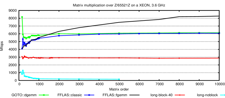
Figure 1: Blocking classical matrix multiplication, on a Xeon, 3.6GHz.

Figure 1 shows the advantage of this method (FFLAS::classic) compared to two other implementations: the naive algorithm (long-noblock), and a hand-made cache tuned implementation, based on block decomposition of the input matrices, so that each block product could be performed locally in the L2 cache memory (long-block-40, for a block dimension $40$). The graph compares the computation speed in millions of field operations per seconds (Mfops) for different matrix orders. As a comparison we also provide the computation speed of the equivalent numerical BLAS routine dgemm. This approach improves on the efficiency of the two other methods over a finite field and the overhead of the modular reductions is limited. Finally, the (FFLAS::fgemm) implementation is the most efficient thanks to the combination of numerical computations and a fast matrix multiplication algorithm which is discussed in the next section.

3.2 Winograd fast algorithm

The third feature of this kernel is the use of a fast matrix multiplication algorithm. We will focus on Winograd’s variant [24, algorithm 12.1] of Strassen’s algorithm [45]. We denote by $\text{MM}(n)$ the dominant term of the arithmetic complexity of the matrix multiplication. The value of $\text{MM}(n)$ thus reflects the choice of algorithm, e.g. $\text{MM}(n)=2n^{3}$ for the classical algorithm, and mean that the actual complexity of the classical algorithm is $2n^{3}+{\cal O}(n^{2})$. We also denote by $\omega$ the asymptotic exponent of $\text{MM}(n)$, it is thus $3$ for the classical algorithm, $\log_{2}(7)\approx 2.807354922$ for the Strassen-Winograd variant, and the best known exponent is about $2.375477$ by [7].

In [30] Winograd’s variant is discarded for numerical computations because of its bad stability and despite its better running time. In [35] aggregation-cancellation techniques of [36] are also compared. They also give better stability than the Winograd variant but worse running time. For exact computation, stability is no longer an issue and Winograd’s faster variant is thus preferred.

3.2.1 A Cascade structure

Asymptotically, this algorithm improves on the number of arithmetic operations required for matrix multiplication from $\text{MM}(n)=2n^{3}$ to $\text{MM}(n)=6n^{2.8074}$. But for a given $n$, the total number of arithmetic operations can be reduced by switching after a few recursive levels of Winograd’s algorithm to the classic algorithm. Table 1 compares the number of arithmetic operations depending on the matrix order and the number of recursive levels.

		Recursive levels of Winograd’s algorithm
$n$	Classic	1	2	3	4	5	6
4	112	144	214
8	960	1024	1248	1738
16	7936	7680	8128	9696	13126
32	64512	59392	57600	60736	71712	95722
64	520192	466944	431104	418560	440512	517344	685414

Table 1: Number of arithmetic operations in the multiplication of two $n\times n$ matrices

This phenomenon is amplified by the fact that additions in classic matrix multiplication are cheaper than the ones in Winograd algorithm since they take advantage of the cache optimization of the BLAS routine. As a consequence, the optimal number of recursive levels depends on the architecture and must be determined experimentally. It can be described by a simple parameter: the matrix order $w$ for which one recursive level is as fast the classic algorithm. Then the number of levels $l$ is given by the formula

$$l=\left\lfloor\text{log}_{2}\frac{n}{w}\right\rfloor+1.$$

3.2.2 Schedule of the algorithm

We based our implementation of Winograd’s algorithm on two different schedules. For the operation $C\leftarrow A\times B$ we use that of [12, Fig. 1] and for the extended $C\leftarrow\alpha A\times B+\beta C$, that of [32, Fig. 6] that we recall in table 2. More details about tasks scheduling and memory efficient variants of Winograd’s algorithm can be found in [21].

#	operation	loc.	#	operation	loc.
1	$S_{1}=A_{21}+A_{22}$	$X_{1}$	12	$S_{4}=A_{12}-S_{2}$	$X_{1}$
2	$T_{1}=B_{12}-B_{11}$	$X_{2}$	13	$T_{4}=T_{2}-B_{21}$	$X_{2}$
3	$P_{5}=\alpha S_{1}T_{1}$	$X_{3}$	14	$C_{12}=\alpha S_{4}B_{22}+C_{12}$	$C_{12}$
4	$C_{22}=P_{5}+\beta C_{22}$	$C_{22}$	15	$U_{5}=U_{2}+C_{12}$	$C_{12}$
5	$C_{12}=P_{5}+\beta C_{12}$	$C_{12}$	16	$P_{4}=\alpha A_{12}T_{4}-\beta C_{21}$	$C_{21}$
6	$S_{2}=S_{1}-A_{11}$	$X_{1}$	17	$S_{3}=A_{11}-A_{21}$	$X_{1}$
7	$T_{2}=B_{22}-T_{1}$	$X_{2}$	18	$T_{3}=B_{22}-B_{12}$	$X_{2}$
8	$P_{1}=\alpha A_{11}B_{11}$	$X_{3}$	19	$U_{3}=\alpha S_{3}T_{3}+U_{2}$	$X_{3}$
9	$C_{11}=P_{1}+\beta C_{11}$	$C_{11}$	20	$U_{7}=U_{3}+C_{22}$	$C_{22}$
10	$U_{2}=\alpha S_{2}T_{2}+P_{1}$	$X_{3}$	21	$U_{6}=U_{3}-C_{21}$	$C_{21}$
11	$U_{1}=\alpha A_{12}B_{21}+C_{11}$	$C_{11}$

Table 2: Schedule for operation $C\leftarrow\alpha A\times B+\beta C$ with 3 temporaries

3.2.3 Control of the overflow

Since Winograd’s algorithms will be used with delayed modular reductions, one has to ensure that any intermediate computation will fit in the underlying fixed-size integer representation being used. Indeed, intermediate values can become large in this algorithm, and the former bound for the dot-product no-longer holds.

The main result of this section is that, in the worst case, the largest intermediate computation occurs during the recursive computation of the sixth recursive product $P_{6}$ (see appendix A). This result generalizes [17, theorem 3.1] for the computation of $AB+\beta C$.

Theorem 3.1.

Let $A\in\mathbb{Z}^{m\times k}$, $B\in\mathbb{Z}^{k\times n}$ $C\in\mathbb{Z}^{m\times n}$ be three matrices and $\beta\in\mathbb{Z}$ with $m_{A}\leq a_{i,j}\leq M_{A}$, $m_{B}\leq b_{i,j}\leq M_{B}$ and $m_{C}\leq c_{i,j}\leq M_{C}$. Moreover, suppose that $0\leq-m_{A}\leq M_{A}$, $0\leq-m_{B}\leq M_{B}$, $0\leq-m_{C}\leq M_{C}$, $M_{C}\leq M_{B}$ and $|\beta|\leq M_{A},M_{B}$. Then every intermediate value $z$ involved in the computation of $A\times B+\beta C$ with $l$ ($l\geq 1$) recursive levels of Winograd algorithm satisfy:

$$\left|z\right|\leq\left(\frac{1+3^{l}}{2}M_{A}+\frac{1-3^{l}}{2}m_{A}\right)\left(\frac{1+3^{l}}{2}M_{B}+\frac{1-3^{l}}{2}m_{B}\right)\left\lfloor{\frac{k}{2^{l}}}\right\rfloor$$

Moreover, this bound is optimal.

The proof is given in appendix A.

Using a positive integer representation of the prime field elements (integers between $0$ and $p-1$), the following corollary holds:

Corollary 3.2 (Positive modular representation).

Using the same notations, with $a_{i,j},b_{i,j},c_{i,j},\beta\in[0\dots p-1]$, we have

$$\left|z\right|\leq\left(\frac{1+3^{l}}{2}\right)^{2}\left\lfloor{\frac{k}{2^{l}}}\right\rfloor(p-1)^{2}$$

Instead, using a balanced representation (integers between $-\frac{p-1}{2}$ and $\frac{p-1}{2}$), this bound can be improved:

Corollary 3.3 (Balanced modular representation).

Using the same notations with $a_{i,j},b_{i,j},c_{i,j},\beta\in[-\frac{p-1}{2}\dots\frac{p-1}{2}]$, we have

$$\left|z\right|\leq\left(\frac{3^{l}}{2}\right)^{2}\left\lfloor{\frac{k}{2^{l}}}\right\rfloor\left(p-1\right)^{2}$$

Corollary 3.4.

One can compute $l$ recursive levels of Winograd algorithm without modular reduction over integers of $\gamma$ bits as long as $k<k_{\text{Winograd}}$ where

$$k_{\text{Winograd}}=\left(\frac{2^{\gamma+2}}{\left((1+3^{l})(p-1)\right)^{2}}+1\right)2^{l}$$

for a positive modular representation and

$$k_{\text{Winograd}}=\left(\frac{2^{\gamma+2}}{\left(3^{l}(p-1)\right)^{2}}+1\right)2^{l}$$

for a balanced modular representation.

3.3 Timings and comparison with numerical routines

This section presents experiments of our implementation of the matrix multiplication kernel described above.

The experiments use two different BLAS library: the automatically tuned BLAS ATLAS [46], and the BLAS by Kazushige Goto [28] refered to as GOTO. We used the gcc compiler version 4.1 on the Xeon machine and the icc compiler version 9.0 on the Itanium. We recall that dgemm refers to the BLAS matrix multiplication routine over double precision floating point numbers. Similarly, we named our routine over a word-size finite field fgemm.

		$n$	1000	2000	3000	5000	7000	8000	9000	10000
		fgemm	$0.38$s	$2.73$s	$8.59$s	$36.34$s	$95.21$	$134.03$s	$190.21$s	$258.08$
		dgemm	$0.37$s	$2.98$s	$10.02$s	$46.10$s	$126.38$s	$188.97$s	$267.83$s	$368.30$s
	ATLAS	$\frac{fgemm}{dgemm}$	1.02	0.92	0.86	0.79	0.75	0.71	0.71	0.70
		fgemm	$0.36$s	$2.53$s	$7.95$s	$33.44$s	$87.46$s	$124.86$s	$177.25$s	$238.00$s
		dgemm	$0.34$s	$2.65$s	$8.90$s	$41.01$s	$112.31$s	$167.20$s	$237.16$s	$325.62$s
	GOTO	$\frac{fgemm}{dgemm}$	1.05	0.96	0.89	0.82	0.78	0.75	0.75	0.73

Table 3: Comparison between fgemm and dgemm on a Xeon, 3.6GHz

		$n$	1000	2000	3000	5000	7000	8000	9000	10000
		fgemm	$0.46$s	$3.22$s	$10.14$s	$42.28$s	$110.64$s	$163.53$s	$225.08$s	$296.56$s
		dgemm	$0.45$s	$3.49$s	$11.45$s	$53.12$s	$144.45$s	$215.53$s	$305.21$s	$419.00$s
	ATLAS	$\frac{fgemm}{dgemm}$	1.01	0.92	0.89	0.80	0.77	0.76	0.74	0.71
		fgemm	$0.43$s	$2.99$s	$9.35$s	$39.21$s	$104.07$s	$152.12$s	$209.22$s	$277.32$s
		dgemm	$0.40$s	$3.18$s	$10.61$s	$48.88$s	$133.75$s	$200.11$s	$283.94$s	$390.37$s
	GOTO	$\frac{fgemm}{dgemm}$	1.06	0.94	0.88	0.80	0.78	0.76	0.74	0.71

Table 4: Comparison between fgemm and dgemm on Itanium2, 1.3GHz

The tables 3 and 4 report timings obtained for both exact and numeric matrix multiplication. First the comparison shows that the exact computation over a word size finite field (modulo 65521 on these tables) can reach a similar range of efficiency as the numerical computation. For increasing matrix dimensions, the exact computation becomes even more efficient (see also figure 1), thanks to the use of Winograd’s algorithm (improvement factor between $13\%$ and $29\%$ for dimension $10\,000$).

These experiments also show the advantage of relying on a generic interface for numerical BLAS: the exact computation will directly take advantage of the improvements of the best numerical routine. This appears when comparing GOTO and ATLAS on these two target architecture, where GOTO is about $10\%$ faster.

4 Triangular system solving with matrix right/left hand side

We now discuss the implementation of solvers for triangular systems with matrix right hand side (or equivalently left hand side). The resolution of such systems plays a central role in many linear algebra problems, e.g. it is the second main operation in block Gaussian elimination after matrix multiplication as will be recalled in section 5.1. This operation is commonly named trsm in the BLAS convention. In the following, we will consider without loss of generality the resolution of an upper triangular system with matrix right hand side, i.e. the operation $B\leftarrow U^{-1}B$, where $U$ is $m\times m$ upper triangular and $B$ is $m\times n$.

Following the approach of the BLAS numerical routine, our implementation is based on a block recursive algorithm to reduce the computation to matrix multiplications.

Now similarly to our approach with matrix multiplication, the design of our implementation also focuses on delaying the modular reductions as much as possible. As will be shown in section 4.2, delaying the whole resolution leads to a quick growth in the size of coefficients. Therefore we also present in section 4.3 another way of delaying these modular reductions. We lastly present how to combine these two techniques within a multi-cascade algorithm.

4.1 The block recursive algorithm

Algorithm trsm recalls the block recursive algorithm.

Data: $A\in\leavevmode\kern 1.00006pt\raise 0.0pt\hbox{$\mathbb{Z}$}\kern-1.00006pt/\kern-1.49994pt\lower 1.29167pt\hbox{p}\mbox{$\mathbb{Z}$}^{m\times m}$, $B\in\leavevmode\kern 1.00006pt\raise 0.0pt\hbox{$\mathbb{Z}$}\kern-1.00006pt/\kern-1.49994pt\lower 1.29167pt\hbox{p}\mbox{$\mathbb{Z}$}^{m\times n}$.

Result: $X\in\leavevmode\kern 1.00006pt\raise 0.0pt\hbox{$\mathbb{Z}$}\kern-1.00006pt/\kern-1.49994pt\lower 1.29167pt\hbox{p}\mbox{$\mathbb{Z}$}^{m\times n}$ such that $AX=B$.

begin  if $m=1$ then  $X:=A_{1,1}^{-1}\times B$

else  /* splitting matrices into two blocks of sizes $\left\lfloor\frac{m}{2}\right\rfloor$ and $\left\lceil\frac{m}{2}\right\rceil$ $$\begin{array}[]{cccc}A&X&&B\\ \overbrace{\left[\begin{array}[]{cc}A_{1}&A_{2}\\ &A_{3}\end{array}\right]}&\overbrace{\left[\begin{array}[]{ccc}&X_{1}&\\ &X_{2}&\end{array}\right]}&=&\overbrace{\left[\begin{array}[]{ccc}&B_{1}&\\ &B_{2}&\end{array}\right]}\end{array}$$ */

$X_{2}:=$trsm ($A_{3},B_{2}$)

$B_{1}:=B_{1}-A_{2}X_{2}$

$X_{1}:=$trsm ($A_{1},B_{1}$)

  end

Algorithm 1 trsm ($A,B$)

Lemma 4.1.

Algorithm trsm is correct and the leading term of its arithmetic complexity over $\leavevmode\kern 1.00006pt\raise 0.0pt\hbox{$\mathbb{Z}$}\kern-1.00006pt/\kern-1.49994pt\lower 1.29167pt\hbox{p}\mbox{$\mathbb{Z}$}$ is

$$\text{TRSM}(m,n)=\frac{1}{2^{\omega-1}-2}\left\lceil\frac{n}{m}\right\rceil\text{MM}(m)$$

This complexity is $m^{2}n$ using classic matrix multiplication.

Proof.

Extending the previous notation MM (n), we denote by MM (m,k,n) the cost of multiplying a $m\times k$ by a $k\times n$ matrices. The cost function $\text{TRSM}(m,n)$ satisfies the following equation:

$$\text{TRSM}(m,n)=2\text{TRSM}(\frac{m}{2},n)+\text{MM}(\frac{m}{2},\frac{m}{2},n).$$

Let $t=\log_{2}(m)$. Although the algorithm works for any $n$, we restrict the complexity analysis to the case where $m\leq n$ for the sake of simplicity. We then have:

$$\text{TRSM}(m,n) = 2\text{TRSM}(\frac{m}{2},n)+\frac{1}{2^{\omega-1}}\left\lceil\frac{n}{m}\right\rceil\text{MM}(m)$$

$$= 2^{t}\text{TRSM}(1,n)+\frac{1}{2^{\omega-1}}\left\lceil\frac{n}{m}\right\rceil\text{MM}(m)\frac{1-\left(\frac{2}{2^{\omega-1}}\right)^{t}}{1-\frac{2}{2^{\omega-1}}}.$$

As $\text{TRSM}(1,n)=2n$ and $\left(2^{\omega-1}\right)^{t}=m^{\omega-1}$, we obtain the expected complexity $\text{TRSM}(m,n)=\frac{1}{2^{\omega-1}-2}\left\lceil\frac{n}{m}\right\rceil\text{MM}(m)+{\cal O}(m^{2}+mn).$ ∎

4.2 Delaying reductions globally

As for matrix multiplication, the delayed computation relies on the fact that ring operations over the finite field can be replaced by ring operations over $\mathbb{Z}$ using the ring homomorphisms described in section 2.1.2. However, triangular system resolutions involve, in the general case, field operations: the divisions by the diagonal elements of the triangular matrix. Therefore this technique is only valid with unit diagonal matrices.

In the general case, the triangular matrix is made unit diagonal by the following factorization: $A=DU$, where $D$ is diagonal and $U$ is unit diagonal upper triangular. Then the system $UX=D^{-1}B$ only involves ring operations and can be solved over $\mathbb{Z}$. This normalization leads to an additional cost of $O(mn)$ arithmetic operations (see [18] for more details).

Now the integer computation with a fixed sized arithmetic (e.g. the floating point arithmetic) is exact as long as all intermediate results of the computation do not exceed the bit capacity of the representation. Therefore we now propose bounds on the values computed by the algorithm over $\mathbb{Z}$.

Theorem 4.2.

Let $T\in\mathbb{Z}^{n\times n}$ be a unit diagonal upper triangular matrix and $b\in\mathbb{Z}^{n}$, with $m\leq T_{i,j}\leq M$ and $m\leq b_{i}\leq M$ and $m\leq 0\leq M$. Let $x=(x_{i})_{i\in[1\dots n]}\in\mathbb{Z}^{n}$ be the solution of the system $Tx=b$. Then $\forall\ k\in[0\dots n-1]$ :

$$\left\{\begin{array}[]{ll}-u_{k}\leq x_{n-k}\leq v_{k}&\text{for $k$ even,}\\ -v_{k}\leq x_{n-k}\leq u_{k}&\text{for $k$ odd}\end{array}\right.$$

with

$$\left\{\begin{array}[]{l}u_{k}=\frac{M-m}{2}(M+1)^{k}-\frac{M+m}{2}(M-1)^{k},\\ v_{k}=\frac{M-m}{2}(M+1)^{k}+\frac{M+m}{2}(M-1)^{k}.\\ \end{array}\right.$$

Proof.

First note the following relations:

$$\forall k\left\{\begin{array}[]{lcl}u_{k}&\leq&v_{k}\\ -mu_{k}&\leq&Mv_{k}\\ -mv_{k}&\leq&Mu_{k}\\ \end{array}\right.$$

The third one comes from

$$Mu_{k}+mv_{k}=\frac{M^{2}-m^{2}}{2}((M+1)^{k}-(M-1)^{k})\geq 0.$$

The proof is now an induction on $k$, following the system resolution order. The initial case $k=0$ correspond to the first step: $x_{n}=b_{n}$, leading to

$$-u_{0}=m\leq x_{n}\leq M=v_{0}.$$

Suppose now that the inequalities hold for $k\in[0\dots l]$ and prove them for $k=l+1$. If $l$ is odd, $l+1$ is even.

$$x_{n-l-1} = b_{n-l-1}-\sum_{j=n-l}^{n}{T_{n-l-1,j}x_{j}}$$

$$\leq M+\sum_{i=0}^{\frac{l-1}{2}}{\max(Mu_{2i},-mv_{2i})+\max(Mv_{2i+1},-mu_{2i+1})}$$

$$\leq M\left(1+\sum_{i=0}^{\frac{l-1}{2}}{u_{2i}+v_{2i+1}}\right)$$

$$\leq M\left(1+\sum_{i=0}^{\frac{l-1}{2}}{\frac{M-m}{2}(M+2)(M+1)^{2i}+\frac{M+m}{2}(M-2)(M-1)^{2i}}\right)$$

$$\leq M\left(1+\frac{M-m}{2}(M+2)\frac{(M+1)^{l+1}-1}{(M+1)^{2}-1}+\frac{M+m}{2}(M-2)\frac{(M-1)^{l+1}-1}{(M-1)^{2}-1}\right)$$

$$\leq \frac{M-m}{2}(M+1)^{l+1}+\frac{M+m}{2}(M-1)^{l+1}=v_{l+1}.$$

Similarly,

$$x_{n-l-1} \geq m-\sum_{i=0}^{\frac{l-1}{2}}{\max(Mv_{2i},-mu_{2i})+\max(Mu_{2i+1},-mv_{2i+1})}$$

$$\geq m-M\sum_{i=0}^{\frac{l-1}{2}}{v_{2i}+u_{2i+1}}$$

$$\geq m-M\sum_{i=0}^{\frac{l-1}{2}}{\frac{M-m}{2}(M+2)(M+1)^{2i}-\frac{M+m}{2}(M-2)(M-1)^{2i}}$$

$$\geq m-M\left(\frac{M-m}{2}(M+2)\frac{(M+1)^{l+1}-1}{(M+1)^{2}-1}-\frac{M+m}{2}(M-2)\frac{(M-1)^{l+1}-1}{(M-1)^{2}-1}\right)$$

$$\geq \frac{M-m}{2}(M+1)^{l+1}-\frac{M+m}{2}(M-1)^{l+1}=u_{l+1}.$$

For $l$ even, a similar proof leads to

$$-v_{l+1}\leq x_{n-l-1}\leq u_{l+1}.$$

∎

Corollary 4.3.

Using the notation of theorem 4.2,

$$|x|\leq\frac{M-m}{2}(M+1)^{n-1}+\frac{M+m}{2}(M-1)^{n-1}.$$

Moreover this bound is optimal.

Proof.

The sequence $(v_{k})$ is increasing and always greater than $(u_{k})$. Thus $\forall\ k\in[0\dots n-1]\ |x_{n-k}|\leq\ u_{k}\leq v_{k}\leq v_{n-1}$.

Now the vector $x=(x_{i})_{i\in[1\dots n]}\in\mathbb{Z}^{n}$ such that $\forall\ k\in[0\dots n-1]\ |x_{n-k}|=v_{k}$ satisfies the system $Tx=b$ with

$$T=\ \left[\begin{array}[]{ccccc}\ddots&\ddots&\ddots&\ddots&\ddots\\ &1&M&m&M\\ &&1&M&m\\ &&&1&M\\ &&&&1\\ \end{array}\right],b=\left[\begin{array}[]{c}\vdots\\ m\\ M\\ m\\ M\end{array}\right]$$

Therefore the bound is reached. ∎

The following corollaries apply this result to the positive and balanced modular representations.

Corollary 4.4 (Positive modular representation).

For $1\leq i,j\leq n$, if $T_{i,j},b_{i}\in[0\dots p-1]$, then

$$|x|\leq\frac{p-1}{2}(p^{n-1}+(p-1)^{n-1}).$$

Corollary 4.5 (Balanced modular representation).

For $1\leq i,j\leq n$, if $T_{i,j},b_{i}\in[-\frac{p-1}{2}\dots\frac{p-1}{2}]$, then

$$|x|\leq\frac{p-1}{2}\left(\frac{p+1}{2}\right)^{n-1}.$$

Remark 4.6.

The balanced modular representation improves the bound by a factor of $2^{n-1}$.

As a consequence, one can solve a unit diagonal triangular system of dimension $n$ using arithmetic operations with integers stored on $\gamma$ bits if

$$\frac{p-1}{2}(p^{n-1}+(p-1)^{n-1})<2^{\gamma}$$ (4)

for a positive representation and

$$\frac{p-1}{2}\left(\frac{p+1}{2}\right)^{n}<2^{\gamma}$$ (5)

for a balanced representation.

For instance, using the double floating point representation ($53$ bits of mantissa) the maximal dimension of the system is $34$ (resp. $52$) for a positive (resp. balanced) representation of $\mathbb{Z}_{3}$. For larger fields, this maximal dimension becomes quickly very small: with $p=1001$, $n\leq 5$ (resp. $n\leq 6$) for a positive (resp. balanced) representation.

In the following, we will denote by $t_{\text{del}}(p,\gamma)$ the maximum dimension for the resolution with delayed modular reductions. This dimension is small, and this approach can therefore only be used as a terminal case of the recursive block algorithm. This first cascade algorithm is characterized by the threshold $t_{\text{del}}$. For efficiency, we used in our implementation the BLAS routine trsm to perform the delayed computation over $\mathbb{Z}$. Despite the small dimension of the blocks, we will see in section 4.4 that this approach can slightly improve the efficiency of the computation when the finite field is small.

4.3 Delaying reductions in the update phase only

The block recursive algorithm consists in several matrix multiplications of different dimensions. In most cases, the matrix multiplications are done over $\mathbb{Z}$ with a modular reduction on the result only. But part of these result matrices will be accumulated to other matrix multiplications in later computations. Therefore these intermediate modular reductions could be delayed even more by allowing to accumulate these results over $\mathbb{Z}$ as much as possible.

This technique can be applied within the former cascade algorithm, to produce a double cascade structure. The key idea is to split the matrices at two levels as shown on figure 2:

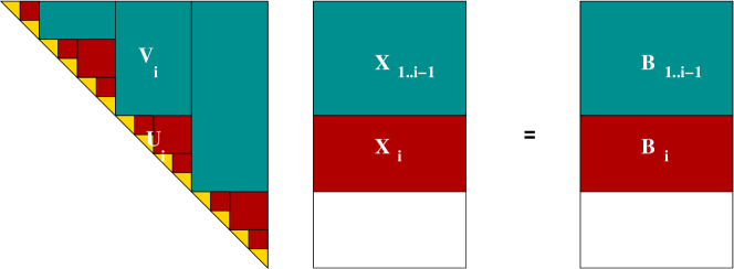
Figure 2: Splitting for the double cascade trsm algorithm

a fine grain splitting with the dimension $t_{\text{del}}$ of the previous section, and a coarse grain splitting with the dimension $t_{\text{update}}$ such that all recursive calls of dimension lower than $t_{\text{update}}$ can let the matrix multiplication updates accumulate without modular reductions. Choosing $t_{\text{update}}=k_{\text{Winograd}}$ (from corrolary 3.4) will ensure this property. To adjust together the dimensions of the two block decompositions, we set $t_{\text{split}}=\left\lfloor t_{\text{Winograd}}/t_{\text{del}}\right\rfloor t_{\text{del}}$.

Data: $A\in\leavevmode\kern 1.00006pt\raise 0.0pt\hbox{$\mathbb{Z}$}\kern-1.00006pt/\kern-1.49994pt\lower 1.29167pt\hbox{p}\mbox{$\mathbb{Z}$}^{m\times m}$, $B\in\leavevmode\kern 1.00006pt\raise 0.0pt\hbox{$\mathbb{Z}$}\kern-1.00006pt/\kern-1.49994pt\lower 1.29167pt\hbox{p}\mbox{$\mathbb{Z}$}^{m\times n}$

Result: $X\in\leavevmode\kern 1.00006pt\raise 0.0pt\hbox{$\mathbb{Z}$}\kern-1.00006pt/\kern-1.49994pt\lower 1.29167pt\hbox{p}\mbox{$\mathbb{Z}$}^{m\times n}$ s.t. $AX=B$

begin  Compute $t_{\text{del}}$ from equation (4 or 5)

Compute $t_{\text{Winograd}}$ from corrolary (3.4)

$t_{\text{split}}=\left\lfloor t_{\text{Winograd}}/t_{\text{del}}\right\rfloor t_{\text{del}}$

foreach block column of $A$ of dimension $m\times t_{\text{split}}$ of the form $\begin{bmatrix}V_{i}\\ U_{i}\\ 0\end{bmatrix}$ do  $X_{i}=\texttt{trsm-partial-delayed}(U_{i},B_{i})$

$X_{i}=X_{i}\mod p$

$B_{1\dots i-1}=B_{1\dots i-1}-V_{i}X_{i}$

$B_{1\dots i-1}=B_{1\dots i-1}\mod p$

  return $X$ end

Algorithm 2 trsm-rec-BLAS-delayed :

Data: $A\in\leavevmode\kern 1.00006pt\raise 0.0pt\hbox{$\mathbb{Z}$}\kern-1.00006pt/\kern-1.49994pt\lower 1.29167pt\hbox{p}\mbox{$\mathbb{Z}$}^{m\times m}$, $B\in\leavevmode\kern 1.00006pt\raise 0.0pt\hbox{$\mathbb{Z}$}\kern-1.00006pt/\kern-1.49994pt\lower 1.29167pt\hbox{p}\mbox{$\mathbb{Z}$}^{m\times n}$, $m$ must be lower than $t_{\text{update}}$

Result: $X\in\leavevmode\kern 1.00006pt\raise 0.0pt\hbox{$\mathbb{Z}$}\kern-1.00006pt/\kern-1.49994pt\lower 1.29167pt\hbox{p}\mbox{$\mathbb{Z}$}^{m\times n}$ s.t. $AX=B$

begin  if $m\leq n_{\text{del}}$ then  $B=B\mod p$

$X=\texttt{dtrsm}(A,B)$ ;  /* the BLAS routine */

$X=X\mod p$

else  /* (splitting of the matrix into blocks of dimension $\left\lfloor\frac{m}{2}\right\rfloor$ and $\left\lceil\frac{m}{2}\right\rceil$) */

$\begin{array}[]{cccc}A&X&&B\\ \overbrace{\left[\begin{array}[]{cc}A_{1}&A_{2}\\ &A_{3}\end{array}\right]}&\overbrace{\left[\begin{array}[]{ccc}&X_{1}&\\ &X_{2}&\end{array}\right]}&=&\overbrace{\left[\begin{array}[]{ccc}&B_{1}&\\ &B_{2}&\end{array}\right]}\end{array}$

$X_{2}:=\texttt{trsm-partial-delayed}(A_{3},B_{2})$

$B_{1}:=B_{1}-A_{2}X_{2}$ ;  /* without modular reduction */

$X_{1}:=\texttt{trsm-partial-delayed}(A_{1},B_{1})$

  return $X$ end

Algorithm 3 trsm-partial-delayed

Algorithm 2 is a loop on every block of column dimension $t_{\text{update}}$. For each of them, the triangular system is solved using algorithm 3 and the update is performed by a matrix multiplication over $\mathbb{Z}$ followed by a modular reduction. Algorithm 3 is simply the cascade algorithm of the previous section: the block recursive algorithm 1 with the fully delayed algorithm as a terminal case. The matrix multiplication updates are performed over $\mathbb{Z}$ without any reduction of the result, since the threshold $t_{\text{update}}$ allows to accumulate them.

4.4 Experiments

We now compare three implementations of the trsm routine over a word size finite field:

Pure recursive (Pure-Rec): Simply algorithm 1,

Recursive-BLAS (Rec-BLAS): The cascade algorithm formed by the recursive algorithm and the BLAS routine dtrsm as a terminal case. It differs from algorithm 3 by the fact that the matrix multiplication $B_{1}:=B_{1}-A_{2}X_{2}$ is always followed by a modular reduction.

Recursive-BLAS-Delayed (Rec-BLAS-Delayed): algorihtm 2.

We compare these three variants over finite fields with different cardinalities, so as to make the parameters $t_{\text{del}}$ and $t_{\text{update}}$ vary as in the following table:

$p$	$\lceil\log_{2}p\rceil$	$t_{\text{del}}$	$t_{\text{update}}$
5	3	23	2 147 483 642
1 048 583	20	2	8190
8 388 617	23	2	126

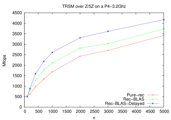
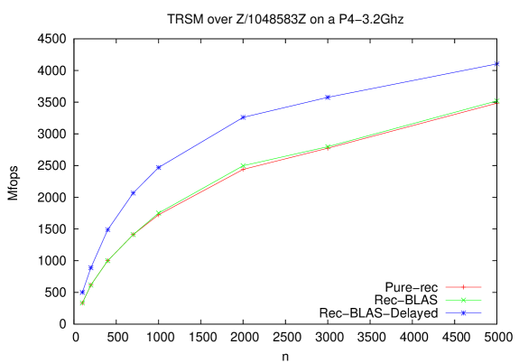
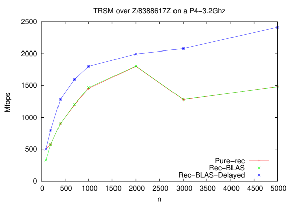
Figure 3: Comparison of the trsm variants for $p=5,1\,048\,583,8\,388\,617$, on a Pentium4-3,2Ghz-1Go

In the experiments of figure 3, the matrix $B$ is square ($m=n$). One can first notice the gain provided by the use of the first cascade with the delayed dtrsm routine by comparing the curves rec-BLAS and pure-rec for $p=5$. This advantage shrinks when the characteristic gets larger, since $t_{\text{del}}=2$ for $p=1\,048\,583$ or $p=8\,388\,61$.

Now the introduction of the coarse grain splitting, delaying the reductions in the update phase improves by up to 500 Mfops the computation speed. This gain is similar for $p=5$ and $p=1\,048\,583$ since in both cases $n<t_{\text{update}}$ and there is therefore no modular reduction between the matrix multiplications.

Lastly for $p=8\,388\,617$, the speed drops down since more reductions are required. The variants pure-rec and rec-BLAS are penalized by their dichotomic splitting, creating too many modular reductions after each matrix multiplication. Now rec-BLAS-delayed has the best efficiency since the double cascade structure minimizes the number of reductions.

We now give a comparison of this implementation with the equivalent routine of the original BLAS dtrsm. As for matrix multiplication in section 3.3, we compare the routines according to two different BLAS implementations (i.e. ATLAS and GOTO) and two different architectures. Nevertheless, we do not present the results with ATLAS on Xeon architecture due to the surprisingly poor efficiency of ATLAS dtrsm during our tests. In the following, ftrsm denotes the trsm routine over $16$-bits prime field (i.e. $\mathbb{Z}_{65521}$) using the ZpZ-double implementation.

		$n$	1000	2000	3000	5000	7000	8000	9000	10000
	ATLAS	ftrsm	$0.37$s	$1.93$s	$5.73$s	$23.63$s	$62.50$s	$91.67$s	$121.84$s	$166.74$s
		ftrsm	$0.25$s	$1.66$s	$5.08$s	$21.47$s	$55.95$s	$80.77$s	$111.57$s	$150.81$s
		dtrsm	$0.17$s	$1.35$s	$4.50$s	$20.64$s	$56.19$s	$83.85$s	$119.18$s	$163.33$s
	GOTO	$\frac{ftrsm}{dtrsm}$	1.47	1.23	1.13	1.04	1.00	0.96	0.94	0.92

Table 5: Timings of triangular solver with matrix hand side on a Xeon, 3.6GHz

		$n$	1000	2000	3000	5000	7000	8000	9000	10000
		ftrsm	$0.34$s	$2.28$s	$7.11$s	$30.26$s	$77.43$s	$112.01$s	$158.00$s	$214.31$s
		dtrsm	$0.26$s	$1.95$s	$6.37$s	$28.60$s	$76.44$s	$113.78$s	$161.19$s	$219.31$s
	ATLAS	$\frac{ftrsm}{dtrsm}$	1.31	1.17	1.12	1.06	1.01	0.98	0.98	0.98
		ftrsm	$0.30$s	$2.00$s	$6.23$s	$26.67$s	$68.22$s	$104.32$s	$137.96$s	$192.37$s
		dtrsm	$0.21$s	$1.61$s	$5.36$s	$24.59$s	$67.35$s	$100.42$s	$142.43$s	$195.79$s
	GOTO	$\frac{ftrsm}{dtrsm}$	1.43	1.24	1.16	1.08	1.01	1.04	0.97	0.98

Table 6: Timings of triangular solver with matrix hand side on Itanium2, 1.3GHz

Tables 6 and 6 show that our implementation of exact trsm solving is not far from numerical performances. Moreover, on our Xeon architecture, with GOTO BLAS, we are able to achieve even better performances than numerical solving for matrices of dimension greater than $7\,000$.

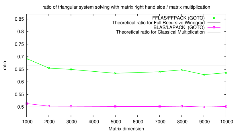
Figure 4: Comparing triangular system solving with matrix multiplication on a Xeon, 3.6GHz

The good performance of our implementation is mostly achieved with the efficient reduction to fast matrix multiplication and the double cascade structure. Figure 4 shows the ratio of the computation time of our trsm compared with matrix multiplication routine. According to lemma 4.1, this ratio is $1/2$ with $\omega=3$ and $2/3$ with $\omega=\log_{2}7$. In practice, our implementation only performs a few recursive calls of Winograd’s algorithm, and the ratio appears to be between $0.5$ and $0.666$ as soon as the dimension is large enough, showing the good efficiency of the reduction to matrix multiplication.

5 Finite Field Matrix Factorizations

We now come to one of the major interest of linear algebra over finite field: matrix multiplication based algorithms. The classical block Gaussian elimination is one of the most common algorithm to achieve a reduction to matrix multiplication [45]. Nevertheless, our main concern here is the singularity of the matrices since we want to derive efficient algorithms for most problems (e.g. rank or nullspace). One approach there is then to use a triangular form of the input matrix. Hence, matrix triangularization algorithm plays a central role for this approach. In this section we focus on practical implementations of triangularization in order to efficiently deal with rank profile, unbalanced dimensions, memory management, recursive thresholds, etc. In particular we demonstrate the efficiency of matrix multiplication reduction in practice for many linear algebra problems.

5.1 Triangularizations

The classical block $LDU$ or $LUP$ factorizations (see [1]) can not be used due to their restriction to non-singular case. Instead one would rather use the LQUP factorization of [33]. We here propose a fully in-place variant and analyze its behaviour.

The LQUP  factorization is a generalization of the well known block LUP  factorization for the singular case [5]. Let $A$ be a $m\times n$ matrix, we want to compute the quadruple $<L,Q,U,P>$ such that $A=LQUP$. The matrix L is lower triangular, P and Q are permutation matrices and U is a rank $r$ upper triangular matrix with its $r$ first rows non-zero.

The algorithm with best known complexity computing this factorization uses a divide and conquer approach and reduces to matrix multiplication [33]. Let us describe briefly the behavior of this algorithm.

The algorithm is recursive: first, it splits $A$ in halves and performs a recursive call on the top half. After some row permutations, It thus gives the $T$, $Y$ and $L_{1}$ blocks of figure 5, together with some row permutations stored in $Q$. Then, after some column permutations ($[XZ]=[A_{21}A_{22}]P$), the algorithm computes $G$ such that $GT=X$ via trsm, replaces $X$ by zeroes and eventually updates $Z=Z-GY$. The third step is a recursive call on $Z$, followed by an update of $Q$. We let the readers refer e.g. to [3, (2.7c)] for further details.

Furthermore, our implementation of LQUP  also uses the trick proposed in [18, §4.2], namely storing $L$ in its compressed form $\tilde{L}$.

This triangularization is thus fully in-place.

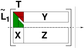
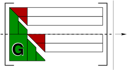
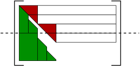
Figure 5: Principle of the LQUP factorization

Lemma 5.1.

The dominant term of the time complexity of algorithm LQUP with $m\leq n$ is

$$\text{LQUP}(m,n)=\left(\left\lceil\frac{n}{m}\right\rceil\frac{1}{2^{\omega-1}-2}-\frac{1}{2^{\omega}-2}\right)\text{MM}(m).$$

The latter is $nm^{2}-\frac{1}{3}m^{3}$ with classical multiplication.

Proof.

Lemma 2.2 ensures that the cost is ${\cal O}(m^{\omega}+nm^{\omega-1})$. We thus just have to look for the constant factors. Then we write $\text{LQUP}(m,n)=\alpha m^{\omega}+\beta nm^{\omega-1}=\text{LQUP}(m/2,n)+\text{TRSM}(m/2,r)+R(m/2,r,n-r)+\text{LQUP}(m/2,n-r)$, where $r$ is the rank of the first $m/2$ rows. This gives $\alpha m^{\omega}+\beta nm^{\omega-1}=\alpha(m/2)^{\omega}+\beta n(m/2)^{\omega-1}+\frac{1}{2^{\omega-1}-2}\left\lceil\frac{m}{2r}\right\rceil\text{MM}(r)+\left\lceil\frac{m(n-r)}{2r^{2}}\right\rceil\text{MM}(r)+\alpha(m/2)^{\omega}+\beta(n-r)(m/2)^{\omega-1}$. With $m\leq n$, the latter is maximal for $r=m/2$, and then, writing $\text{MM}(x)=C_{\omega}x^{\omega}$, we identify the coefficient on both sides: $\beta=\frac{\beta}{2^{\omega-1}}+\frac{C_{\omega}}{2^{\omega-1}}+\frac{\beta}{2^{\omega-1}}$, and $\alpha=2\frac{\alpha}{2^{\omega}}-\frac{\beta}{2^{\omega}}-C_{\omega}\frac{2^{\omega}-6}{2^{\omega}(2^{\omega}-4)}$. Solving for $\beta$ and $\alpha$ gives the announced terms. ∎

5.2 Performance and comparison with numerical routines

Fast matrix multiplication routine of section 3.2 allowed us to speed up matrix multiplication as well as triangular system solving. These improvements are of great interest since they directly improve efficiency of triangularization. We now compare our exact triangularization over finite field with numerical triangularization provided within LAPACK library [2]. In particular, we use an optimized version of this library provided by ATLAS software in which we use two different BLAS kernel: ATLAS and GOTO.

		$n$	1000	2000	3000	5000	7000	8000	9000	10000
		lqup	$0.32$s	$1.84$s	$4.89$s	$19.34$s	$48.94$s	$73.86$s	$97.50$s	$131.11$s
		dgetrf	$0.17$s	$1.19$s	$3.83$s	$16.90$s	$45.32$s	$67.44$s	$94.83$s	$130.15$s
	ATLAS	$\frac{lqup}{dgetrf}$	1.88	1.55	1.28	1.14	1.08	1.10	1.03	1.01
		lqup	$0.25$s	$1.52$s	$4.47$s	$17.93$s	$44.54$s	$67.88$s	$89.63$s	$119.65$s
		dgetrf	$0.15$s	$1.03$s	$3.33$s	$14.84$s	$39.58$s	$58.61$s	$82.89$s	$113.47$s
	GOTO	$\frac{lqup}{dgetrf}$	1.67	1.48	1.34	1.21	1.13	1.16	1.08	1.05

Table 7: Performance of matrix triangularization (for $\leavevmode\kern 1.00006pt\raise 0.0pt\hbox{$\mathbb{Z}$}\kern-1.00006pt/\kern-1.49994pt\lower 1.29167pt\hbox{65521}\lower 1.29167pt\hbox{$\mathbb{Z}$}$ and floats) on a Xeon, 3.6GHz

		$n$	1000	2000	3000	5000	7000	8000	9000	10000
		lqup	$0.38$s	$2.20$s	$6.36$s	$25.22$s	$61.64$s	$89.74$s	$127.43$s	$163.68$s
		dgetrf	$0.20$s	$1.47$s	$4.61$s	$20.26$s	$53.57$s	$79.37$s	$111.66$s	$152.42$s
	ATLAS	$\frac{lqup}{dgetrf}$	1.85	1.50	1.38	1.25	1.15	1.13	1.14	1.07
		lqup	$0.34$s	$2.00$s	$5.81$s	$23.11$s	$56.80$s	$83.90$s	$113.66$s	$150.82$s
		dgetrf	$0.16$s	$1.17$s	$3.80$s	$17.07$s	$46.18$s	$69.00$s	$97.56$s	$134.01$s
	GOTO	$\frac{lqup}{dgetrf}$	2.21	1.72	1.53	1.35	1.23	1.22	1.16	1.13

Table 8: Performance of matrix triangularization (for $\leavevmode\kern 1.00006pt\raise 0.0pt\hbox{$\mathbb{Z}$}\kern-1.00006pt/\kern-1.49994pt\lower 1.29167pt\hbox{65521}\lower 1.29167pt\hbox{$\mathbb{Z}$}$ and floats) on Itanium2-1.3GHz

Tables 8 and 8 show efficiency obtained with our exact triangularization based on fast matrix multiplication and the one obtained with numerical computation. There, “dgetrf” computes a floating point LU factorization of a general $m\times n$ matrix using partial pivoting with row interchanges. Exact computation is done in the prime field of integers modulo $65521$. We are now mostly able to reach the speed of numerical computations. More precisely, we are able to compute the triangularization of a $10\,000\times 10\,000$ matrix over a finite field in about $2$ minutes on a Xeon 3.6GHz architecture. This is only $5\%$ slower than the best numerical computation.

We could have expected that our speed would have been even better than numerical approach since we take advantage of Strassen-Winograd’s multiplication while numerical computations are not. However, in practice we do not fully benefit from fast matrix multiplication since we work at most with matrices of half dimension of the input matrix due to the recursive structure of the algorithm. Then, the number of Winograd calls is at least one less than within matrix multiplication routines. In our tests, it appears that we only use 3 calls on our Xeon architecture and 1 call on the Itanium2 architecture according to matrix multiplication threshold. This explains the better performance on the Xeon compared to numerical routines than the Itanium2 architecture.

Note also that in order to take even more into account data locality one can develop a version of LQUP where blocks are maintained as square as possible. Indeed, as soon as the RAM is full, data locality becomes more important than memory saves. The TURBO method [22] addresses this issue. A first implementation of TURBO has been studied in [18, §4.5] and it reveals to be the fastest for large matrices, despite its bigger memory demand [18, Figure 6]. This is advocating further uses of recursive blocked data formats and of more recursive levels of TURBO.

5.3 Comparison with the multiplication

The LQUP factorization and the trsm routines reduce to matrix multiplication as we have seen in the previous sections. Theoretically, as classic matrix multiplication requires $2n^{3}-n^{2}$ arithmetic operations, the factorization, requiring at most $\frac{2}{3}n^{3}$ arithmetic operations, could be computed in about $\frac{1}{3}$ of the time. However, when Winograd fast matrix multiplication algorithm is used this ratio becomes $\frac{2}{5}$. Figure 6 shows that the experimental behavior of the factorization is not very far from this theoretical ratio.

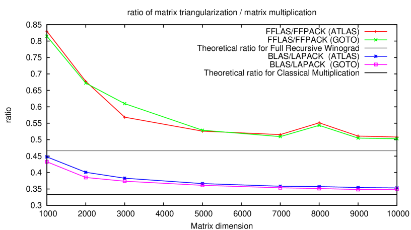
Figure 6: Comparing matrix triangularization with matrix multiplication on a Xeon, 3.6GHz

6 Applications

In this section, we use our matrix multiplication, matrix factorization and matrix solvers as basic routines to perform other linear algebra routines. For instance, from the two routines (i.e. LQUP and trsm), one can also directly derive several other algorithms, e.g.:

• The rank is the number of non-zero rows in $U$.

• The determinant is the product of the diagonal elements of $U$ (stopping whenever a zero is encountered).

In the following, we first give the theoretical complexities with explicit constant terms. These constants depend on the kind of matrix multiplication used (fast or classical). In order to validate our approach we then compare this theoretical ratios to some experimental ones.

6.1 Nullspace basis

Computing a right nullspace basis with the LQUP factorization is immediate on a $m\times n$ full rank matrix, where $m\leq n$: if $U=[U_{1}U_{2}]$, the matrix $U_{1}^{-1}U_{2}$ completed with identity matrix yields a basis for the nullspace of $A$.

This requires $NS(m;n)=LQUP(m;n)+\text{TRSM}(m;n-m)$. which gives

$$NS(m;n)=(\left\lceil\frac{n}{m}\right\rceil\frac{2}{2^{\omega-1}-2}-\frac{1}{2^{\omega}-2})\text{MM}(m)$$ (6)

The latter is $(m^{2}n-\frac{1}{3}m^{3})+(n-m)m^{2}=2m^{2}n-\frac{4}{3}m^{3}$ with classical multiplication. One can notice that computing a right nullspace of the transposed of the input matrix yields a left nullspace basis.

6.2 Triangular multiplications

6.2.1 Triangular matrix multiplication

To perform the multiplication of a triangular matrix by a dense matrix via a block decomposition in halves, one requires four recursive calls and two dense matrix-matrix multiplications. The cost is thus $TRMM(n)=4TRMM(n/2)+2\text{MM}(n/2)$, solving for $TRMM(n)=\alpha\text{MM}(n)$ yields

$$TRMM(n)=\frac{1}{2^{\omega-1}-2}\text{MM}(n).$$ (7)

The latter is $n^{3}$ with classical multiplication.

6.2.2 Upper-lower Triangular matrix multiplication

The block multiplication of a lower triangular matrix by an upper triangular matrix is

$$\begin{array}[]{ccccc}\left[\begin{array}[]{cc}A_{1}&A_{2}\\ &A_{4}\end{array}\right]&\times&\left[\begin{array}[]{cc}B_{1}&\\ B_{3}&B_{4}\end{array}\right]&=&\left[\begin{array}[]{cc}A_{1}B_{1}+A_{2}B_{3}&A_{2}B_{4}\\ A_{4}B_{3}&A_{4}B_{4}\end{array}\right]\end{array}$$

The cost is thus $\text{UTLT}(n)=2\text{UTLT}(n/2)+2TRMM(n/2)+\text{MM}(n/2)$, solving for $\text{UTLT}(n)=\alpha\text{MM}(n)$ yields

$$\text{UTLT}(n)=\frac{2^{\omega}}{(2^{\omega}-4)(2^{\omega}-2)}\text{MM}(n).$$ (8)

The latter is $\frac{2}{3}n^{3}$ with classical multiplication.

6.2.3 Upper-Upper Triangular matrix multiplication

Now the block version is even simpler (of course the lower lower multiplication is similar):

$$\begin{array}[]{ccccc}\left[\begin{array}[]{cc}A_{1}&A_{2}\\ &A_{4}\end{array}\right]&\times&\left[\begin{array}[]{cc}B_{1}&B_{2}\\ &B_{4}\end{array}\right]&=&\left[\begin{array}[]{cc}A_{1}B_{1}&A_{1}B_{2}+A_{2}B_{4}\\ &A_{4}B_{4}\end{array}\right]\end{array}$$

The cost is thus $\text{UTUT}(n)=2\text{UTUT}(n/2)+2TRMM(n/2)$, which yields

$$\text{UTUT}(n)=\frac{4}{(2^{\omega}-4)(2^{\omega}-2)}\text{MM}(n).$$ (9)

The latter is $\frac{1}{3}n^{3}$ with classical multiplication.

6.3 Squaring

6.3.1 $A\times A^{T}$

Suppose we want to compute $A$ times its transpose, even with a diagonal in the middle. The block version is

$$\left[\begin{array}[]{cc}A_{1}&A_{2}\\ A_{3}&A_{4}\end{array}\right]\times\left[\begin{array}[]{cc}D_{1}&\\ &D_{4}\end{array}\right]\times\left[\begin{array}[]{cc}A_{1}^{T}&A_{3}^{T}\\ A_{2}^{T}&A_{4}^{T}\end{array}\right]=\left[\begin{array}[]{cc}A_{1}D_{1}A_{1}^{T}+A_{2}D_{4}A_{2}^{T}&A_{1}D_{1}A_{3}^{T}+A_{2}D_{4}A_{4}^{T}\\ A_{3}D_{1}A_{1}^{T}+A_{4}D_{4}A_{2}^{T}&A_{3}D_{1}A_{3}^{T}+A_{4}D_{4}A_{4}^{T}\end{array}\right]$$

Since $ADA^{T}$ is symmetric, the lower left and upper right are just transpose of one another. The other corners (upper left and lower right) are computed via recursive calls. Thus the arithmetic cost of this special product is $AAT(n)=4AAT(n/2)+2\text{MM}(n/2)+3\text{ADD}(n/2)+2(n/2)^{2}$

Ignoring the cost of the three additions and the diagonal multiplications, this yields

$$AAT(n)=\frac{2}{2^{\omega}-4}\text{MM}(n).$$ (10)

The latter is $n^{3}$ with classical multiplication. One can note that when $A$ is rectangular with $m\leq n$ the cost extends to

$$AAT(m;n)=\left\lceil\frac{n}{m}\right\rceil\frac{2}{2^{\omega}-4}\text{MM}(m).$$ (11)

6.3.2 Symmetric case

When $A$ is already symmetric, and if the diagonal is unitary, the constant factor decreases. Indeed, in this case $A_{2}=A_{3}^{T}$ and then one of the four recursive calls is saved. Also one of the remaining three recursive calls is a call to a non symmetric $AA^{T}$. Therefore the cost is now: $SymAAT(n)=2SymAAT(n/2)+AAT(n/2)+2\text{MM}(n/2)$, once again ignoring $n^{2}$. This yields

$$SymAAT(n)=\frac{2(2^{\omega}-3)}{(2^{\omega}-4)(2^{\omega}-2)}\text{MM}(n).$$ (12)

The latter is $\frac{5}{6}n^{3}$ with classical multiplication.

6.3.3 Triangular case

We here view the explicit computation of $L^{T}DL$ for instance as a special case of upper-lower triangular matrix multiplication, but where both matrices are symmetric of one another. We also show that we can add an extra diagonal factor in the middle at a negligible cost. Consider then

$$\begin{array}[]{ccccccc}\left[\begin{array}[]{cc}L_{1}&\\ L_{3}&L_{4}\end{array}\right]&\times&\left[\begin{array}[]{cc}D_{1}&\\ &D_{4}\end{array}\right]&\times&\left[\begin{array}[]{cc}L_{1}^{T}&L_{3}^{T}\\ &L_{4}^{T}\end{array}\right]&=&\left[\begin{array}[]{cc}L_{1}D_{1}L_{1}^{T}&L_{1}D_{1}L_{3}^{T}\\ L_{3}D_{1}L_{1}^{T}&L_{3}D_{1}L_{3}^{T}+L_{4}D_{4}L_{4}^{T}\end{array}\right]\end{array}$$

Thus it requires two recursive calls, a call to AAT (with a diagonal in the middle) only one call to TRMM as both lower-left and upper-right corners are transpose of one another. This yields

$$\text{LTL}(n)=\frac{4}{(2^{\omega}-4)(2^{\omega}-2)}\text{MM}(n).$$ (13)

The latter is $\frac{1}{3}n^{3}$ with classical multiplication.

6.4 Symmetric factorization

For the sake of simplicity, we here consider the $LU$ factorization of a generic rank profile symmetric $n\times n$ matrix $A$. We could describe how to perform this decomposition with the permutation and the possible rank deficiency in the blocks, but we here only analyze the cost of such a $LDL^{T}$ factorization. The idea is that one can recursively decompose $A=\left[\begin{array}[]{cc}A_{1}&A_{2}\\ A_{2}^{T}&A_{4}\end{array}\right]=\left[\begin{array}[]{cc}L_{1}&\\ G&L_{2}\end{array}\right]\times\left[\begin{array}[]{cc}D_{1}&\\ &D_{2}\end{array}\right]\times\left[\begin{array}[]{cc}L_{1}^{T}&G^{T}\\ &L_{2}^{T}\end{array}\right]$. Well, this requires a recursive call to compute $L_{1}$ and $D_{1}$ ; a TRSM to compute $G$ such that $L_{1}D_{1}G^{T}=A_{2}$ ; an AAT to compute $GD_{1}G^{T}$ and a recursive call to compute $L_{2}D_{2}L_{2}^{T}=A_{4}-GD_{1}G^{T}$. The cost is thus $LDLT(n)=2LDLT(n/2)+\text{TRSM}(n/2)+AAT(n/2)$, which yields

$$LDLT(n)=\frac{4}{(2^{\omega}-4)(2^{\omega}-2)}\text{MM}(n).$$ (14)

The latter is $\frac{1}{3}n^{3}$ with classical multiplication.

6.5 Matrix inverse

6.5.1 Triangular matrix inverse

To invert a triangular matrix via a block decomposition, one requires two recursive calls and two triangular matrix multiplications.

$$\begin{array}[]{ccc}\left[\begin{array}[]{cc}A_{1}&A_{2}\\ &A_{4}\end{array}\right]^{-1}&=&\left[\begin{array}[]{cc}A_{1}^{-1}&-A_{1}^{-1}A_{2}A_{4}^{-1}\\ &A_{4}^{-1}\end{array}\right]\end{array}$$

The cost is thus $\text{INVT}(n)=2\text{INVT}(n/2)+2TRMM(n/2)$ which yields

$$\text{INVT}(n)=\frac{2}{2^{\omega}-2}TRMM(n)=\frac{4}{(2^{\omega}-4)(2^{\omega}-2)}\text{MM}(n).$$ (15)

The latter is $\frac{1}{3}n^{3}$ with classical multiplication.

6.5.2 Matrix inverse

To invert a dense matrix, one needs to compute an $LQUP$ decomposition, then to invert $L$ and permute it with $Q^{-1}$. A TRSM is then required to solve $UX=Q^{-1}L^{-1}$. Applying $P^{-1}$ to X yields the inverse. The cost is then $INV(n)=LQUP(n)+\text{INVT}(n)+\text{TRSM}(n)$. This gives

$$INV(n)=\frac{3\times 2^{\omega}}{(2^{\omega}-4)(2^{\omega}-2)}\text{MM}(n).$$ (16)

The latter is $INV(n)=2n^{3}$ with classical multiplication.

6.5.3 Symmetric inverse

If $A$ is symmetric, one can decompose it into a $LDL^{T}$ factorization instead of the $LU$. Therefore, its inverse is then only one $INVT$ for both $L^{-1}$ and $L^{-T}$ followed by an $LTL$. The cost is then $SymINV(n)=LDLT(n)+\text{INVT}(n)+\text{LTL}(n)$ which yields

$$SymINV(n)=\frac{12}{(2^{\omega}-2)(2^{\omega}-4)}\text{MM}(n).$$ (17)

The latter is $SymINV(n)=n^{3}$ with classical multiplication.

6.5.4 Full-rank Moore-Penrose pseudo-inverse

$A$ is a rectangular full rank $m\times n$ matrix. We suppose, without loss of genericity, that $m\leq n$. The Moore-Penrose inverse of $A$ is thus $A^{\dagger}=A^{T}(AA^{T})^{-1}$, see e.g. [42] and references therein. Computing the Moore-Penrose inverse is then just a $LDL^{T}$ decomposition of the symmetric matrix $AA^{T}$, followed by two rectangular system solvings:

$$MPINV(m;n)=AAT(m;n)+LDLT(m)+2\text{TRSM}(m;n).$$

The cost is then

$$MPINV(m;n)=\left(\left\lceil\frac{n}{m}\right\rceil\frac{6}{2^{\omega}-4}+\frac{4}{(2^{\omega}-2)(2^{\omega}-4)}\right)\text{MM}(m)$$ (18)

The latter is $3m^{2}n+\frac{1}{3}m^{3}$ with classical multiplication. This correspond e.g. to the normal equations numerical resolution [27, algorithm 5.3.1].

6.5.5 Rank deficient Moore-Penrose pseudo-inverse

In this case, one needs to compute a full-rank decomposition of $A$. This is done by performing the $LQUP$ decomposition of $A$ and if $A$ is of rank $r$, selecting the first $r$ columns of $L$ (call them $L_{r}=\left[\begin{array}[]{c}L_{1}\\ G\end{array}\right]$) and the first $r$ rows $U$ (call them $U_{r}=[U_{1}|Y]$), forgetting the permutation $P$. We have $A=L_{r}U_{r}$ and we modify the formula [39, (7)] as follows:

$$A^{\dagger}=\left[\begin{array}[]{c}I\\ Y^{T}U_{1}^{-T}\end{array}\right]\left((L_{1}+L_{1}^{-T}G^{T}G)(U_{1}+YY^{T}U_{1}^{-1})\right)^{-1}[I|L_{1}^{-T}G^{T}].$$ (19)

We note $W=(L_{1}+L_{1}^{-T}G^{T}G)(U_{1}+YY^{T}U_{1}^{-1})$. We compute $W$ by two squarings, two TRSM and a classical matrix multiplication. We perform a reversed LU decomposition on $W$ to get $W=U_{w}L_{w}$. Now we compute $L_{1}^{T}U_{w}$ and $L_{w}U_{1}^{T}$ by upper-upper triangular multiplication and $H=(L_{1}^{T}U_{w})^{-1}G^{T}$ and $Z=Y^{T}(L_{w}U_{1}^{T})^{-1}$ by two TRSM. Now, $A^{\dagger}=\left[\begin{array}[]{cc}W^{-1}&L_{w}^{-1}H\\ ZU_{w}^{-1}&ZH\end{array}\right]$. $W^{-1}$ is two triangular inverses and an upper lower product. $ZH$ is a rectangular multiplication and the last two blocks are obtained by two triangular solvings.

$$MPINV_{r}(m;n)=\text{LQUP}(m;n)+AAT(r;m-r)+AAT(r;n-r)+3\text{TRSM}(r,m-r)\\ +3\text{TRSM}(r,n-r)+\text{MM}(r)+\text{LQUP}(r)+2\text{UTUT}(r)+2\text{INVT}(r)+\text{UTLT}(r)\\ +R(n-r;r;m-r)$$ (20)

The latter is $2rmn+2r^{2}m+2r^{2}n+m^{2}n-\frac{1}{3}m^{3}-\frac{4}{3}r^{3}$ with classical multiplication. To get an idea, numerical computations based on the Cholesky factorization of $AA^{T}$ presented in [8] as faster than SVD or QR or iterative methods would require $3m^{2}n+2r^{2}m+3r^{3}$ flops.

6.5.6 Performances and comparisons with numerical routines

As for triangular system solving and matrix triangularization, we now compare performances of matrix inversion for triangular and dense matrices with numerical computation and with matrix multiplication. Our comparison with numerical computation is still based on LAPACK library with two different BLAS kernel (i.e. ATLAS and GOTO). We do not present the result of triangular matrix inversion over our Xeon architecture according to the bad behavior of “dtrsm” function which is the main routine used by LAPACK for triangular matrix inversion. Our base field is the prime field of integers modulo $65521$ using a Zpz-double representation and we use fast matrix multiplication of section 3.2.

		$n$	1000	2000	3000	5000	7000	8000	9000	10000
	ATLAS	tri. inv	$0.11$s	$0.70$s	$2.17$s	$9.21$s	$24.21$s	$35.53$s	$49.95$s	$68.26$s
		tri. inv	$0.10$s	$0.62$s	$1.90$s	$8.00$s	$20.97$s	$30.77$s	$43.38$s	$58.98$
		dtrtri	$0.18$s	$1.04$s	$2.90$s	$10.97$s	$26.85$s	$38.57$s	$52.93$s	$70.95$s
	GOTO	$\frac{tri.inv}{dtrtri}$	0.56	0.60	0.66	0.73	0.78	0.80	0.82	0.83

Table 9: Timings of triangular matrix inversion on a Xeon, 3.6GHz

		$n$	1000	2000	3000	5000	7000	8000	9000	10000
		tri. inv	$0.19$s	$1.03$s	$3.02$s	$11.91$s	$31.71$s	$44.43$s	$61.37$s	$82.55$s
		dtrtri	$0.08$s	$0.58$s	$2.55$s	$11.39$s	$30.50$s	$44.52$s	$63.34$s	$85.19$s
	ATLAS	$\frac{tri.inv}{dtrtri}$	2.25	1.77	1.18	1.05	1.04	1.00	0.97	0.97
		tri. inv	$0.15$s	$0.85$s	$2.47$s	$10.10$s	$26.10$s	$38.29$s	$53.65$s	$72.74$s
		dtrtri	$0.08$s	$0.61$s	$1.96$s	$8.77$s	$23.68$s	$35.73$s	$49.84$s	$69.10$s
	GOTO	$\frac{tri.inv}{dtrtri}$	1.90	1.40	1.26	1.15	1.10	1.07	1.08	1.05

Table 10: Timings of triangular matrix inversion on Itanium2, 1.3GHz

Tables 10 and 10 illustrate the performances of our exact triangular matrix inversion regarding performances of LAPACK routine “dtrtri”. Results show that our exact computations tend to catch up with the numerical ones and even outperform them on Itanium2 with ATLAS for large matrices (dimension greater than 8000).

One can notice that the implementation of triangular matrix inversion provided by GOTO is quite efficient compare to ATLAS, and thus lead our exact computation to be more efficient but not better than numerical ones. Here again, this demonstrates that exact triangular matrix inversion over finite field is not much more costly than its numerical counterpart.

		$n$	1000	3000	5000	7000	8000	9000	10000
		inverse	$0.75$s	$13.57$s	$54.52$s	$141.19$s	$206.26$s	$285.19$s	$385.35$s
		dgetrf+dgetri	$0.69$s	$16.94$s	$80.83$s	$222.07$s	$368.66$s	$531.29$s	$761.28$s
	ATLAS	$\frac{inverse}{dgetrf+dgetri}$	1.09	0.80	0.67	0.64	0.56	0.54	0.51
		inverse	$0.63$s	$11.82$s	$48.56$s	$125.30$s	$179.17$s	$256.12$s	$343.91$s
		dgetrf+dgetri	$0.55$s	$13.02$s	$58.36$s	$159.21$s	$232.30$s	$328.55$s	$450.46$s
	GOTO	$\frac{inverse}{dgetrf+dgetri}$	1.15	0.91	0.83	0.79	0.77	0.78	0.76

Table 11: Timings of matrix inversion on a Xeon, 3.6GHz

		$n$	1000	3000	5000	7000	8000	9000	10000
		inverse	$1.01$s	$17.27$s	$69.24$s	$173.21$s	$256.67$s	$353.02$s	$483.08$s
		dgetrf+dgetri	$0.60$s	$14.29$s	$66.08$s	$184.74$s	$276.09$s	$393.62$s	$541.37$s
	ATLAS	$\frac{inverse}{dgetrf+dgetri}$	1.67	1.21	1.05	0.94	0.93	0.90	0.89
		inverse	$0.85$s	$14.92$s	$61.00$s	$153.78$s	$226.68$s	$313.84$s	$422.78$s
		dgetrf+dgetri	$0.47$s	$11.45$s	$51.33$s	$139.00$s	$207.36$s	$293.02$s	$402.72$s
	GOTO	$\frac{inverse}{dgetrf+dgetri}$	1.80	1.30	1.19	1.11	1.09	1.07	1.05

Table 12: Timings of matrix inversion on Itanium2, 1.3GHz

Now, Tables 12 and 12 provide the same comparisons for dense matrix inversion. For numerical computation references we use the routine “dgetri” in combination with the factorization routine “dgetrf” to yield matrix inverse. On both architecture with ATLAS BLAS kernel, exact computations become the most efficient when matrix dimension is getting larger. Numerical computation is only better than exact on the Itanium 2 architecture with GOTO BLAS kernel. In this particular application, the benefit of fast matrix multiplication is important since it allows to outperform numerical performances.

As shown in previous section, matrix inversion algorithms reduce to matrix multiplication. Figures 8 and 8 show the correlation between matrix inversion performances and matrix multiplication performances; triangular and dense case are studied.

According to section 6.5.1, the ratio of triangular matrix inversion and matrix multiplication is $4/(2^{\omega}-4)(2^{\omega}-2)$; which gives a theoretical ratio of $1/6$ when classic matrix multiplication is used. However this ratio increase to $\approx 0.267$ when Winograd fast matrix multiplication is used (i.e. $\omega=\log_{2}7$). Since our matrix multiplication routine is using fast matrix multiplication, the asymptotic behavior of this ratio should tend to the latter. However we observe in practice that our performances are beyond this ratio. This is due to the hybrid matrix multiplication which uses both Winograd and classic algorithms. So the practical ratio obtained here is really close to the theoretical one since it should asymptotically lie between $0.2674$ and $0.166$.

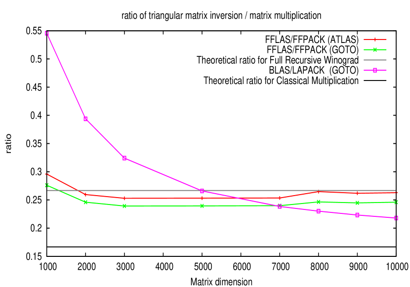
Figure 7: Comparing triangular matrix inversion with matrix multiplication on a Xeon, 3.6GHz

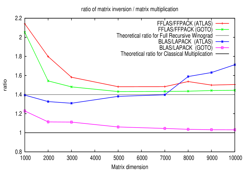
Figure 8: Comparing matrix inversion with matrix multiplication on a Xeon, 3.6GHz

From section 6.5.2 one can express the ratio between dense matrix inversion and matrix multiplication as respectively $1$ with classic algorithm and $1.4$ with Winograd algorithm. In practice we observe that dense matrix inversion ratio is just above the asymptotic behavior of Winograd based inversion. This certainly could be explained by the number of different algorithms involved in this application. In particular it involves three different reductions to matrix multiplications; which may be of a little influence on the final performances. Moreover, we do not take into account memory effect which can play a crucial role in performances as already demonstrated by ATLAS software with optimized BLAS [46]. In our test we used a naive approach which leads us to use $2n^{2}$ elements in memory. Decreasing this memory will certainly allow us to get better performances. In particular, it is not known yet how to perform matrix inversion in place using a reduction to matrix multiplication.

7 Conclusions

We have achieved the goal of approaching the efficiency of the numerical linear algebra library but for word-size prime fields. We showed that exact computation can benefit from Winograd fast matrix multiplication algorithm and then even leads to outperform the efficiency of the well known BLAS and LAPACK libraries.

This performance is achieved through efficient reduction to matrix multiplication where we took care of minimizing the ratio and also by reusing the numerical computation as much as possible. We also showed that from our routines one can easily implement efficient algorithms for many linear algebra problems (e.g. null-space, generalized inverse, etc.). Note that approximate timings for these algorithms can be derived from the timings provided with our main routines.

One can try to design block algorithms where the blocks fit in the cache of a specific machine to reach very good efficiency. By reusing BLAS library this has been proven to be almost useless for matrix multiplication in [17] and we think we proved here that this is not mandatory also for any dense linear algebra routine. Therefore, using recursive block algorithms, efficient numerical BLAS and fast matrix multiplication algorithms one can approach the numerical performance or even surpass them over some finite fields. Moreover, long range efficiency and portability are warranted as opposed to every day tuning. Except for small matrices where the conversions increase slightly the running time, and except for the LQUP transform, we have shown that all our exact routines can be faster than their numerical counterparts.

Besides, the exact equivalent of stability constraints for numerical computations is coefficient growth. Therefore, whenever possible, we computed and improved theoretical bounds on this growth (e.g. bounds 4.5 and 3.3). Those optimal bounds enable further uses of the BLAS routines.

Further developments include:
$\bullet~{}$ The main case where our wrapping of BLAS is insufficient is for very small matrices where benefits of BLAS are limited and fast algorithms are not useful. Here, a design using the finite field directly might improve the speed.
$\bullet~{}$ More generally, a Self-adapting Software [10] would allow to provide hybrid implementations with best empirical thresholds.
$\bullet~{}$ The technique of wrapping BLAS becomes useless when finite fields are larger than the corresponding bound of feasibility (e.g. $p>2^{26}$ for matrix multiplication). At a non negligible price the Chinese remainder algorithm could be used to authorize the use of BLAS. Optimizing this scheme would then be an interesting way to provide similar results for larger finite fields.
$\bullet~{}$ Finally, extending the out of core versions by more recursive data format and the building of a parallel library is promising. Also, in the case of parallelism, our all-recursive approach enables a very efficient “sequential-first” parallelization as shown e.g. in [19] for triangular system solving.

Appendix A Proof of theorem 3.1

Consider the natural block decomposition

$$\begin{bmatrix}C_{11}&C_{12}\\ C_{21}&C_{22}\\ \end{bmatrix}=\begin{bmatrix}A_{11}&A_{12}\\ A_{21}&A_{22}\\ \end{bmatrix}\begin{bmatrix}B_{11}&B_{12}\\ B_{21}&B_{22}\\ \end{bmatrix},$$

where $A_{11}$ and $B_{11}$ have respectively dimension $m/2\times k/2$ and $k/2\times n/2$.

To bound the intermediate values in the computation of $l$ recursive levels of Winograd’s algorithm, we will show that the worst case occurs in the computation of one of the intermediaite products. We will first consider the case $K=2^{l}q$ and then generalize the result for every $K$. To end the proof we will provide an instance of a computation for which the bound is attained.

A.1 Some properties on the series of the type $2u-v$

Consider the series defined recursively by:

$$\left\{\begin{array}[]{l}u_{l+1}=2u_{l}-v_{l}\\ v_{l+1}=2v_{l}-u_{l}\\ u_{0}\leq 0\\ v_{0}\geq 0\\ \end{array}\right.$$

Since

$$\left\{\begin{array}[]{l}u_{l+1}+v_{l+1}=u_{l}+v_{l}=\dots=u_{0}+v_{0}\\ v_{l+1}-u_{l+1}=3(v_{l}-u_{l})=\dots=3^{l+1}(v_{0}-u_{0})\\ \end{array}\right.$$

It comes

$$\left\{\begin{array}[]{l}u_{l}=u_{0}\frac{(1+3^{l})}{2}+v_{0}\frac{(1-3^{l})}{2}\\ v_{l}=v_{0}\frac{(1+3^{l})}{2}+u_{0}\frac{(1-3^{l})}{2}\end{array}\right.$$

Thus, the following properties hold:

$$u_{l}\leq 0~{}\text{and}~{}v_{l}\geq 0$$ (21)

$$u_{l}~{}\text{is decreasing and}~{}v_{l}~{}\text{ is increasing}$$ (22)

$$v_{l}>-u_{l}~{}\text{if}~{}v_{0}>-u_{0}$$ (23)

Now define $v^{A}$ and $v^{B}$, two series of the type $v$ by setting $u^{A}_{0}=m_{A}$, $v^{A}_{0}=M_{A}$, $u^{B}_{0}=m_{B}$ and $v^{B}_{0}=M_{B}$.

Let us also define $t_{j}=\frac{1+3^{j}}{2}$ and $s_{j}=\frac{1-3^{j}}{2}$. Thus $t_{j}+s_{j}=1$ and $t_{j}-s_{j}=3^{j}$.

The following property holds:

$$(2M_{A}-m_{A})t_{j}+(2m_{A}-M_{A})s_{j}=M_{A}t_{j+1}+m_{A}s_{j+1}=v^{A}_{j+1}$$ (24)

A.2 Notations

Let

$$b_{l}=\left(\frac{1+3^{l}}{2}M_{A}+\frac{1-3^{l}}{2}m_{A}\right)\left(\frac{1+3^{l}}{2}M_{B}+\frac{1-3^{l}}{2}m_{B}\right)\left\lfloor{\frac{K}{2^{l}}}\right\rfloor.$$

The serie $(b_{l})_{l>0}$ is increasing since (22).

Winograd’s implementation, see e.g. [32, 21], uses the following intermediate computations

$$P_{1} = A_{11}\times B_{11}$$

$$P_{2} = A_{12}\times B_{21}+\beta C_{11}$$

$$P_{3} = (A_{12}+A_{11}-A_{21}-A_{22})\times B_{22}$$

$$P_{4} = A_{22}\times(B_{22}+B_{11}-B_{21}-B_{12})+\beta(C_{22}-C_{12}-C_{21})$$

$$P_{5} = (A_{21}+A_{22})\times(B_{12}-B_{11})+\beta C_{12}$$

$$P_{6} = (A_{21}+A_{22}-A_{11})\times(B_{22}+B_{11}-B_{12})$$

$$P_{7} = (A_{11}-A_{21})\times(B_{22}-B_{12})+\beta(C_{22}-C_{12})$$

$$C_{11}=U_{1} = P_{2}+P_{1}$$

$$U_{2} = (A_{21}+A_{22}-A_{11})\times(B_{22}-B_{12})+(A_{21}+A_{22})\times B_{11}$$

$$U_{3} = A_{22}\times(B_{22}-B_{12})+(A_{21}+A_{22})\times B_{11}+\beta(C_{22}-C_{12})$$

$$U_{4} = (A_{21}+A_{22})\times B_{22}+A_{11}\times(B_{12}-B_{22})+\beta C_{12}$$

$$C_{12}=U_{5} = U_{4}+P_{3}$$

$$C_{21}=U_{6} = U_{3}-P_{4}$$

$$C_{22}=U_{7} = U_{3}+P_{5}$$

Remark that the result of the computation is independent of the algorithm and is always bounded by $K\text{max}(|m_{A}|,|M_{A}|)\text{max}(|m_{B}|,|M_{B}|)+\beta\text{max}(|m_{C}|,|M_{C}|)\leq(K+1)M_{A}M_{B}$. Now this value is always smaller than $b_{1}$ for $k\geq 1$ and also smaller than $b_{l}\ \forall l\geq 1$. Therefore, the coefficients of the blocks $U_{1}$, $U_{5}$, $U_{6}$ and $U_{7}$ always satisfy the bound. Now if the remaining 9 intermediate computations are bounded by $b_{l}$, we will be done.

We will prove that the largest intermediate value always occurs in the computation of $P_{6}$. Consider $l$ recursive levels indexed by $j$: $j=l$ is the first splitting of the matrices into four blocks and $j=0$ corresponds to the last level where the product is done by a classic matrix multiplication algorithm. The recursive algorithm can be seen as a back and forth process: the splitting is done from $j=l$ to $j=0$ and then the multiplications are done from $j=0$ to $j=l$.

We also define the following notations:

• $M^{j,k}_{m_{A},M_{A},m_{B},M_{B},m_{C},M_{C}}(X)$ is an upper bound on the intermediate computations of $X=A\times B+\beta C$ with $j$ recursive levels and $m_{A}\leq a_{i,j}\leq M_{A}$, $m_{B}\leq b_{i,j}\leq M_{B}$ and $m_{C}\leq c_{i,j}\leq M_{C}$. $k$ is the common dimension of $A$ and $B$

• $M^{j,k}_{m_{A},M_{A},m_{B},M_{B},m_{C},M_{C}}=\max_{X}M^{j,k}_{m_{A},M_{A},m_{B},M_{B},m_{C},M_{C}}(X)$.

• $M(X)\frac{k}{2^{j+1}}$ for $M^{j+1,k}_{m_{A},M_{A},m_{B},M_{B},m_{C},M_{C}}(X)$.

The following formulas correspond to the seven recursive calls:

$$\begin{array}[]{c}M^{j+1,k}_{m_{A},M_{A},m_{B},M_{B},m_{C},M_{C}}=\\ \max{\left(\begin{array}[]{l}M(P_{1})=M^{j,\frac{k}{2}}_{m_{A},M_{A},m_{B},M_{B},0,0}\\ M(P_{2})=M^{j,\frac{k}{2}}_{m_{A},M_{A},m_{B},M_{B},m_{C},M_{C}}\\ M(P_{3})=M^{j,\frac{k}{2}}_{2m_{A}-2M_{A},2M_{A}-2m_{A},m_{B},M_{B},0,0}\\ M(P_{4})=M^{j,\frac{k}{2}}_{m_{A},M_{A},2m_{B}-2M_{B},2M_{B}-2m_{B},m_{C}-2M_{C},M_{C}-2m_{C}}\\ M(P_{5})=M^{j,\frac{k}{2}}_{2m_{A},2M_{A},m_{B}-M_{B},M_{B}-m_{B},m_{C},M_{C}}\\ M(P_{6})=M^{j,\frac{k}{2}}_{2m_{A}-M_{A},2M_{A}-m_{A},2m_{B}-M_{B},2M_{B}-m_{B},0,0}\\ M(P_{7})=M^{j,\frac{k}{2}}_{m_{A}-M_{A},M_{A}-m_{A},m_{B}-M_{B},M_{B}-m_{B},m_{C}-M_{C},M_{C}-m_{C}}\\ \end{array}\right)}\end{array}$$ (25)

Moreover, the classic algorithm is used for $j=0$:

$$M^{0,k}_{m_{A},M_{A},m_{B},M_{B},m_{C},M_{C}}=\text{max}\left(\begin{array}[]{l}M_{A}M_{B}k+\beta M_{C}\\ -m_{A}M_{B}k-\beta m_{C}\\ -M_{A}m_{B}k-\beta m_{C}\\ \end{array}\right)$$ (26)

A.3 Some invariants

Lemma A.1.

The following invariants hold in every recursive call:

1. $0\leq-m_{A}\leq M_{A},\ 0\leq-m_{B}\leq M_{B},\ 0\leq-m_{C}\leq M_{C}$

2. $m_{C}\geq m_{B}$ and $M_{C}\leq M_{B}$

3. $M_{C}-m_{C}\leq M_{B}-m_{B}$

Proof.

From equation (25), one gets invariants ($1$) and ($2$). Then invariant ($3$) is a consequence of ($1$) and ($2$). ∎

A.4 Induction for $K=2^{l}q$

Let $IH_{j}$ be the following induction hypothesis:

If the invariants of section A.3 are satisfied then

$$M^{j,k}_{m_{A},M_{A},m_{B},M_{B},m_{C},M_{C}}=[v^{A}_{j}][v^{B}_{j}]\frac{k}{2^{j}}.$$

Suppose that the previous invariants are satisfied and that $IH_{j}$ is true. We will prove that the maximum of (25) is reached during the computation of $P_{6}$ to show that $IH_{j+1}$ is satisfied.

The conditions on $m_{A}$, $M_{A}$, $m_{B}$ and $M_{B}$ are satisfied for every recursive call. We can therefore apply $IH_{j}$ to every product $X\in\{P_{1},P_{2},P_{3},P_{4},P_{5},P_{6}\}$ in order to compare $M(X)$ with $M(P_{6})$.

• For $P_{1}=A_{11}\times B_{11}$:

  $$M(P_{6})-M(P_{1}) = \left[(2M_{A}-m_{A})t_{j}+(2m_{A}-M_{A})s_{j}\right]\times$$

  $$\left[(2M_{B}-m_{B})t_{j}+(2m_{B}-M_{B})s_{j}\right]-v^{A_{11}}_{j}v^{B_{11}}_{j}$$

  $$= v^{A}_{j+1}v^{B}_{j+1}-v^{A_{11}}_{j}v^{B_{11}}_{j}$$

  $$\geq v^{A}_{j+1}v^{B}_{j+1}-v^{A}_{j}v^{B}_{j}$$

  And since $v^{A}$ and $v^{B}$ are increasing and positive, we have $M(P_{6})\geq M(P_{1})$.

• For $P_{2}=A_{12}\times B_{21}+\beta C_{11}$: with the same argument $M(P_{6})\geq M(P_{2})$.

• For $P_{3}=(A_{12}+A_{11}-A_{21}-A_{22})\times B_{22}$:

  $$M(P_{6})-M(P_{3}) = v^{A}_{j+1}v^{B}_{j+1}-v^{A_{11}+A_{12}-A_{21}-A_{22}}_{j}v^{B_{22}}_{j}$$

  $$= v^{A}_{j+1}v^{B}_{j+1}-[(2M_{A}-2m_{A})t_{j}+(2m_{A}-2M_{A})s_{j}]v^{B}_{j}$$

  $$= v^{A}_{j+1}v^{B}_{j+1}-(v^{A}_{j+1}-m_{A}t_{j}-M_{A}s_{j})v^{B}_{j}(\ref{eq:vap})$$

  $$= v^{A}_{j+1}[v^{B}_{j+1}-v^{B}_{j}]-u^{A}_{j}v^{B}_{j}$$

  $$\geq v^{A}_{j+1}[v^{B}_{j+1}-v^{B}_{j}]-v^{A}_{j+1}v^{B}_{j}(\ref{eq:sup})$$

  $$\geq v^{A}_{j+1}[v^{B}_{j+1}-2v^{B}_{j}]$$

  $$\geq v^{A}_{j+1}3^{j}[M_{B}-m_{B}]\geq 0$$

• For $P_{4}=A_{22}\times(B_{22}+B_{11}-B_{21}-B_{12})+\beta(C_{22}-C_{12}-C_{21})$: with the same argument,

  $$M(P_{6})-M(P_{4})=v^{A}_{j+1}v^{B}_{j+1}-v^{A_{22}}_{j}v^{B_{22}+B_{11}-B_{12}-B_{21}}_{j}\geq 0$$

• For $P_{5}=(A_{21}+A_{22})\times(B_{12}-B_{11})+\beta C_{12}$:

  $$M(P_{6})-M(P_{5}) = v^{A}_{j+1}v^{B}_{j+1}-v^{A_{21}+A_{22}}_{j}v^{B_{12}-B_{11}}_{j}$$

  $$= v^{A}_{j+1}v^{B}_{j+1}-2v^{A}_{j}\left[v_{j}^{B}-u_{j}^{B}\right]$$

  $$= \left[2v^{A}_{j}-u^{A}_{j}\right]v^{B}_{j+1}-v^{A}_{j}\left[v^{B}_{j+1}-u_{j}^{B}\right]$$

  $$= v^{A}_{j}v^{B}_{j+1}-u^{A}_{j}v^{B}_{j+1}+v^{A}_{j}u_{j}^{B}$$

  $$= v^{A}_{j}\left[v^{B}_{j+1}+u_{j}^{B}\right]-u^{A}_{j}v^{B}_{j+1}$$

  $$= v^{A}_{j}\left[2v_{j}^{B}\right]-u^{A}_{j}v^{B}_{j+1}$$

  and since $u^{A}_{j}\leq 0\leq v^{A}_{j},v_{j}^{B},v^{B}_{j+1}$ it comes $M(P_{6})-M(P_{5})\geq 0$.

• For $P_{7}=(A_{11}-A_{21})\times(B_{22}-B_{12})+\beta(C_{22}-C_{12})$: using $P_{5}$,

  $$M(P_{5})-M(P_{7}) = v^{A_{21}+A_{22}}_{j}v^{B_{12}-B_{11}}_{j}-v^{A_{11}-A_{21}}_{j}v^{B_{22}-B_{12}}_{j}$$

  $$= [2M_{A}t_{j}+2m_{A}s_{j}-(M_{A}-m_{A})t_{j}-(m_{A}-M_{A})s_{j}]\times$$

  $$\left[(M_{B}-m_{B})t_{j}+(m_{B}-M_{B})s_{j}\right]$$

  $$= \left[(M_{A}+m_{A})(t_{j}+s_{j})\right]\left[(M_{B}-m_{B})(t_{j}-s_{j})\right]$$

  $$\geq 0$$

  The coefficients of the blocks $U_{1},U_{5},U_{6}$ and $U_{7}$ are bounded by $kM_{A}M_{B}+\beta M_{C}$ and are therefore smaller than the ones in $P_{6}$.

  Lastly, we must control the size of the coefficients in $U_{2}=P_{1}+P_{6}$, $U_{3}=U_{2}+P_{7}$ and $U_{4}=U_{2}+P_{7}$.

• For $U_{2}=(A_{21}+A_{22}-A_{11})\times(B_{22}-B_{12})+(A_{21}+A_{22})\times B_{11}$:

  $$\forall x\in U_{2},|x|\leq\max{\left(\begin{array}[]{l}(2M_{A}-m_{A})(M_{B}-m_{B})+2M_{A}M_{B}\\ (-2m_{A}+M_{A})(M_{B}-m_{B})-2m_{A}M_{B}\\ (-2m_{A}+M_{A})(M_{B}-m_{B})-2M_{A}m_{B}\end{array}\right)}k/2^{j}$$ (27)

  Now $2M_{A}-m_{A}-(-2m_{A}+M_{A})=M_{A}+m_{A}\geq 0$ and $0\leq-m_{A}\leq M_{A}$, so the 27 simplifies into $\forall x\in U_{2},|x|\leq(2M_{A}-m_{A})(M_{B}-m_{B})+2M_{A}M_{B}$.

  $$M(P_{6})-M(U_{2}) \geq (2M_{A}-m_{A})(2M_{B}-m_{B})-(2M_{A}-m_{A})(M_{B}-m_{B})$$

  $$-2M_{A}M_{B}$$

  $$= (2M_{A}-m_{A})(M_{B})-2M_{A}M_{B}$$

  $$= -m_{A}M_{B}\geq 0$$

• For $U_{3}=A_{22}\times(B_{22}-B_{12})+(A_{21}+A_{22})\times B_{11}+\beta(C_{22}-C_{12})$: with the same argument

  $$\forall x\in U_{3},|x|\leq\max{\left(\begin{array}[]{l}(M_{A}(M_{B}-m_{B})+2M_{A}M_{B})k/2^{j}+|\beta|(M_{C}-m_{C})\\ (M_{A}(M_{B}-m_{B})-2m_{A}M_{B})k/2^{j}+|\beta|(M_{C}-m_{C})\\ (M_{A}(M_{B}-m_{B})-2M_{A}m_{B})k/2^{j}+|\beta|(M_{C}-m_{C})\\ \end{array}\right)}k/2^{j}$$

  The max is always equal to its first argument, and since $k/2^{j}\geq 1$, $\beta\leq M_{A}-m_{A}$ and $M_{C}-m_{C}\leq M_{B}-m_{B}$, we have:

  $$|x| \leq (M_{A}(M_{B}-m_{B})+2M_{A}M_{B})k/2^{j}+\beta(M_{C}-m_{C})$$

  $$\leq (2M_{A}-m_{A})(M_{B}-m_{B})+2M_{A}M_{B})k/2^{j}$$

  $$\leq M(U2)\leq M(P6)$$

• For $U_{4}=(A_{21}+A_{22})\times B_{22}+A_{11}\times(B_{12}-B_{22})+\beta C_{12}$: with the same argument as for $U_{3}$,

  $$\forall x\in U_{4},|x|\leq(M_{A}(M_{B}-m_{B})+2M_{A}M_{B})k/2^{j}+|\beta|M_{C}$$

  Since $M_{C}\leq M_{B}-m_{B}$, $-m_{A}\leq M_{A}$ and $-m_{B}\leq M_{B}$, we have

  $$M(U_{4})\leq M(U_{3})\leq M(P_{6}).$$

Finally $M^{j+1,k}_{m_{A},M_{A},m_{B},M_{B}}=M(P_{6})\frac{k}{2^{j+1}}=v^{A}_{j+1}v^{B}_{j+1}\frac{k}{2^{j+1}}$, and $IH_{j+1}$ is satisfied.

For the initialization of the induction ($j=1$), the products of the blocks are done by the classical algorithm. From (25) and (26), one gets:

$$M^{1,k}_{m_{A},M_{A},m_{B},M_{B},m_{C},M_{C}}(P_{1}) = M_{A}M_{B}k/2$$

$$M^{1,k}_{m_{A},M_{A},m_{B},M_{B},m_{C},M_{C}}(P_{2}) = M_{A}M_{B}k/2+|\beta|M_{C}$$

$$M^{1,k}_{m_{A},M_{A},m_{B},M_{B},m_{C},M_{C}}(P_{3}) = 2(M_{A}-m_{A})M_{B}k/2$$

$$M^{1,k}_{m_{A},M_{A},m_{B},M_{B},m_{C},M_{C}}(P_{4}) = 2M_{A}(M_{B}-m_{B})k/2+|\beta|(2M_{C}-m_{C})$$

$$M^{1,k}_{m_{A},M_{A},m_{B},M_{B},m_{C},M_{C}}(P_{5}) = 2M_{A}(M_{B}-m_{B})k/2+|\beta|M_{C}$$

$$M^{1,k}_{m_{A},M_{A},m_{B},M_{B},m_{C},M_{C}}(P_{6}) = (2M_{A}-m_{A})(2M_{B}-m_{B})k/2$$

$$M^{1,k}_{m_{A},M_{A},m_{B},M_{B},m_{C},M_{C}}(P_{7}) = (M_{A}-m_{A})(M_{B}-m_{B})k/2+|\beta|(M_{C}-m_{C})$$

$$M^{1,k}_{m_{A},M_{A},m_{B},M_{B},m_{C},M_{C}}(U_{2}) = (2M_{A}-m_{A})(M_{B}-m_{B})k/2+2M_{A}M_{B}k/2$$

$$M^{1,k}_{m_{A},M_{A},m_{B},M_{B},m_{C},M_{C}}(U_{3}) = M_{A}(M_{B}-m_{B})k/2+2M_{A}M_{B}k/2+|\beta|(M_{C}-m_{C})$$

$$M^{1,k}_{m_{A},M_{A},m_{B},M_{B},m_{C},M_{C}}(U_{4}) = 2M_{A}M_{B}k/2+M_{A}(M_{B}-m_{B})k/2+|\beta|M_{C}$$

Again, we will prove that $M^{1,k}_{m_{A},M_{A},m_{B},M_{B},m_{C},M_{C}}(P_{6})$ reaches the highest value, using invariants of section A.3, and the fact that $|\beta|\leq M_{A},M_{B}$ and $k\geq 2$.

It is straightforward for $P_{1}$ and $P_{2}$.

• For $P_{3}$:

  $$M^{1,k}_{m_{A},\dots}(P_{6})-M^{1,k}_{m_{A},\dots}(P_{3}) = ((2M_{A}-m_{A})(2M_{B}-m_{B})-2(M_{A}-m_{A})M_{B})k/2$$

  $$= (2M_{A}M_{B}k-(2M_{A}-m_{A})m_{B})k/2\geq 0$$

• For $P_{4}$: Since $-|\beta|(2M_{C}-m_{C})\geq-M_{A}(2M_{B}-m_{B})$, we have

  $$M^{1,k}_{m_{A},\dots}(P_{6})-M^{1,k}_{m_{A},\dots}(P_{4}) = ((2M_{A}-m_{A})(2M_{B}-m_{B})-2M_{A}(M_{B}-m_{B}))k/2$$

  $$-|\beta|(M_{C}-2m_{C})$$

  $$\geq (M_{A}-m_{A})(2M_{B}-m_{B})-2M_{A}(M_{B}-m_{B})$$

  $$= m_{A}(m_{B}-2M_{B})\geq 0$$

• For $P_{5}$: $M^{1,k}_{m_{A},M_{A},m_{B},M_{B},m_{C},M_{C}}(P_{5})\leq M^{1,k}_{m_{A},M_{A},m_{B},M_{B},m_{C},M_{C}}(P_{4})$

• For $P_{7}$:

  $$M^{1,k}_{m_{A},\dots}(P_{6})-M^{1,k}_{m_{A},\dots}(P_{7}) = ((2M_{A}-m_{A})(2M_{B}-m_{B})$$

  $$-(M_{A}-m_{A})(M_{B}-m_{B})k/2-|\beta|(M_{C}-m_{C})$$

  $$\geq M_{A}(2M_{B}-m_{B})+(M_{A}-m_{A})M_{B}-M_{A}(M_{B}-m_{B})$$

  $$\geq (2M_{A}-m_{A})M_{B}\geq 0$$

• For $U_{2}$, $U_{3}$, $U_{4}$: using the same argument as for the case of arbitrary $j$.

$IH_{1}$ is then satisfied.

A.5 Case of an arbitrary $k$

Let $l$ be such that $2^{l}d\leq k<2^{l}(d+1)$ ( $d=\left\lfloor\frac{k}{2^{l}}\right\rfloor$). A dynamic peeling technique [31] is used to deal with odd dimensions: at each recursive level, the largest blocks with even dimensions at the top left hand corner of the input matrices are multiplied using Winograd’s algorithm. Then an optional rank $1$ update is applied, with the odd dimensions.

These updates are using matrix-vector products, dot products and tensor products. Every intermediate result during these computations are therefore bounded in absolute value by $kM_{A}M_{B}+|\beta|M_{C}\leq(k+1)M_{A}M_{B}$

We show now that this bound is always under the one of Winograd’s algorithm.

$$\forall l\geq 1\ 2^{l}(d+1)M_{A}M_{B}\leq v_{l}^{A}v_{l}^{B}\left\lfloor\frac{k}{2^{l}}\right\rfloor$$

(since $(k+1)M_{A}M_{B}\leq 2^{l}(d+1)M_{A}M_{B}$).

• For $l=1$, the inequation is satisfied: $2M_{A}M_{B}(d+1)\leq(2M_{A}-m_{A})(2M_{B}-m_{B})d$ (since $d\geq 1$)

• Let us suppose that it is satisfied for $l\geq 1$ and prove it for $l+1$:

  $$v_{l+1}^{A}v_{l+1}^{B}\left\lfloor\frac{k}{2^{l+1}}\right\rfloor = [(2M_{A}-m_{A})t_{l}+(2m_{A}-M_{A})s_{l}]$$

  $$\times [(2M_{B}-m_{B})t_{l}+(2m_{B}-M_{B})s_{l}]d$$

  $$\geq 2[M_{A}t_{l}+m_{A}s_{l}][M_{B}t_{l}+m_{B}s_{l}]2d$$

  $$\geq v_{l}^{A}v_{l}^{B}\left\lfloor\frac{k}{2^{l}}\right\rfloor$$

  $$\geq 2(2^{l}M_{A}M_{B}(2d+1))$$

  $$\geq 2^{l+1}M_{A}M_{B}(d+1))$$

By induction, the bound of section A.4 is valid for any $k$.

A.6 Optimality of the bound

We simply build a sequence of square matrices $A_{l}$ and $B_{l}$ of order $2^{l}$ for which $l$ recursive calls to Winograd’s algorithm will involve intermediate results equals to the bound.

Let $(A_{l})_{l\in\mathbb{N}^{*}}$ and $(B_{l})_{l\in\mathbb{N}^{*}}$ be recursively defined as follows:

$$\left\{\begin{array}[]{rr}A_{1}=\left[\begin{array}[]{cc}m_{A}&0\\ M_{A}&M_{A}\end{array}\right],&B_{1}=\left[\begin{array}[]{cc}M_{B}&m_{B}\\ 0&M_{B}\end{array}\right]\\ &\\ A_{l+1}=\left[\begin{array}[]{cc}\overline{A_{l}}&0\\ A_{l}&A_{l}\end{array}\right],&B_{l+1}=\left[\begin{array}[]{cc}B_{l}&\overline{B_{l}}\\ 0&B_{l}\end{array}\right]\end{array}\right.$$

where $\overline{A_{i,j}}=M_{A}+m_{A}-A_{i,j}$ and $\overline{B_{i,j}}=M_{B}+m_{B}-B_{i,j}$.

Since at each recursive level, the computation of $P6=(A_{21}+A_{22}-A_{11})\times(B_{22}+B_{11}-B_{12})$ involves the largest possible intermediate values, let us define:

$$S(A_{l})=(A_{l})_{2,1}+(A_{l})_{2,2}-(A_{l})_{1,1}=2A_{l-1}-\overline{A_{l-1}}=3A_{l-1}-J_{l-1}$$

where $J_{k}$ is the square matrix of order $2^{k}$ whose coefficients are all equals to $M_{A}+m_{A}$.

Moreover $S(J_{k})=J_{k-1}$. Thus, applying $P_{6}$ $l$ times recursively, since $S$ is linear:

$$S(S(\ldots(S(A_{l}))))=S^{l}(A_{l})=3^{l-1}S(A_{1})-\left(\sum_{k=0}^{l-2}3^{k}\right)J_{1}$$

Then $S(A_{1})=2M_{A}-m_{A}$ and $J_{1}=M_{A}+m_{A}$ imply:

$$S^{l}(A_{l})=3^{l-1}(2M_{A}-m_{A})-\frac{3^{l-1}-1}{3-1}(M_{A}+m_{A})=\frac{1+3^{l}}{2}M_{A}+\frac{1-3^{l}}{2}m_{A}.$$

The same holds for $B_{l}$:

$$S^{l}(B_{l})=\frac{1+3^{l}}{2}M_{B}+\frac{1-3^{l}}{2}m_{B}$$

The order of $A_{l}$ and $B_{l}$ is $k=2^{l}$, so $\left\lfloor\frac{k}{2^{l}}\right\rfloor=1$. Therefore, the computation of $A_{l}\times B_{l}$ with $l$ recursive levels of Winograd’s algorithm involves intermediate values equals to $v_{l}^{A_{l}}v_{l}^{B_{l}}\left\lfloor\frac{k}{2^{l}}\right\rfloor$. This proves the optimality of the bound.

Note that this bound is unchanged for computations of the type $A\times B+\beta C$.

References

- [1] Alfred V. Aho, John E. Hopcroft, and Jeffrey D. Ullman. The Design and Analysis of Computer Algorithms. Addison-Wesley, 1974.
- [2] E. Anderson, Z. Bai, C. Bischof, S. Blackford, J. Demmel, J. Dongarra, J. Du Croz, A. Greenbaum, S. Hammarling, A. McKenney, and D. Sorensen. LAPACK Users’ Guide. Society for Industrial and Applied Mathematics, Philadelphia, PA, third edition, 1999.
- [3] Dario Bini and Victor Pan. Polynomial and Matrix Computations, Volume 1: Fundamental Algorithms. Birkhauser, Boston, 1994.
- [4] Morgan Brassel, Pascal Giorgi, and Clement Pernet. LUdivine: A symbolic block LU factorisation for matrices over finite fields using blas, April 2003. Poster, http://ljk.imag.fr/membres/Jean-Guillaume.Dumas/FFLAS/FFLAS_Download/lu%divine_poster_eccad2003.ps.gz.
- [5] James R. Bunch and John E. Hopcroft. Triangular factorization and inversion by fast matrix multiplication. Mathematics of Computation, 28:231–236, 1974.
- [6] Zhuliang Chen and Arne Storjohann. Effective reductions to matrix multiplication, July 2003. ACA’2003, 9th International Conference on Applications of Computer Algebra, Raleigh, North Carolina State University, USA.
- [7] Don Coppersmith and Shmuel Winograd. Matrix multiplication via arithmetic progressions. Journal of Symbolic Computation, 9(3):251–280, 1990.
- [8] Pierre Courrieu. Fast computation of Moore-Penrose inverse matrices. Neural Information Processing - Letters and Reviews, 8(2):25–29, August 2005.
- [9] John D. Dixon. Exact solution of linear equations using p-adic expansions. Numerische Mathematik, 40:137–141, 1982.
- [10] Jack Dongarra and Victor Eijkhout. Self-adapting numerical software and automatic tuning of heuristics. Lecture Notes in Computer Science, 2660:759–770, January 2003.
- [11] Jack J. Dongarra, Jeremy Du Croz, Sven Hammarling, and Iain Duff. A set of level 3 Basic Linear Algebra Subprograms. Transactions on Mathematical Software, 16(1):1–17, March 1990. http://doi.acm.org/10.1145/77626.79170.
- [12] C. C. Douglas, M. Heroux, G. Slishman, and R. M. Smith. Gemmw: A portable level 3 blas winograd variant of strassen’s matrix-matrix multiply algorithm. Journal of Computational Physics, 110:1–10, 1994.
- [13] Jean-Guillaume Dumas, , Pascal Giorgi, and Clément Pernet. FFLAS-FFPACK: Finite field linear algebra subroutine/package. Software, http://ciel.ccsd.cnrs.fr/ciel-00000025, February 2006.
- [14] Jean-Guillaume Dumas. Efficient dot product over finite fields. In Victor G. Ganzha, Ernst W. Mayr, and Evgenii V. Vorozhtsov, editors, Proceedings of the seventh International Workshop on Computer Algebra in Scientific Computing, Yalta, Ukraine, pages 139–154. Technische Universität München, Germany, July 2004.
- [15] Jean-Guillaume Dumas. Q-adic transform revisited. Technical Report 0710.0510 [cs.SC], ArXiv, October 2007. http://hal.archives-ouvertes.fr/hal-00173894.
- [16] Jean-Guillaume Dumas, Thierry Gautier, Mark Giesbrecht, Pascal Giorgi, Bradford Hovinen, Erich Kaltofen, B. David Saunders, Will J. Turner, and Gilles Villard. LinBox: A generic library for exact linear algebra. In Arjeh M. Cohen, Xiao-Shan Gao, and Nobuki Takayama, editors, Proceedings of the 2002 International Congress of Mathematical Software, Beijing, China, pages 40–50. World Scientific Pub, August 2002.
- [17] Jean-Guillaume Dumas, Thierry Gautier, and Clément Pernet. Finite field linear algebra subroutines. In Teo Mora, editor, Proceedings of the 2002 International Symposium on Symbolic and Algebraic Computation, Lille, France, pages 63–74. ACM Press, New York, July 2002.
- [18] Jean-Guillaume Dumas, Pascal Giorgi, and Clément Pernet. FFPACK: Finite field linear algebra package. In Jaime Gutierrez, editor, Proceedings of the 2004 International Symposium on Symbolic and Algebraic Computation, Santander, Spain, pages 119–126. ACM Press, New York, July 2004.
- [19] Jean-Guillaume Dumas, Clément Pernet, and Jean-Louis Roch. Adaptive triangular system solving. In Challenges in Symbolic Computation Software, October 2006. Dagstuhl Seminar proceedings 06271, paper 770.
- [20] Jean-Guillaume Dumas, Clément Pernet, and Zhendong Wan. Efficient computation of the characteristic polynomial. In Manuel Kauers, editor, Proceedings of the 2005 International Symposium on Symbolic and Algebraic Computation, Beijing, China, pages 140–147. ACM Press, New York, July 2005.
- [21] Jean-Guillaume Dumas, Clément Pernet, and Wei Zhou. Memory efficient scheduling of Strassen-Winograd’s matrix multiplication algorithm. Technical report, arXiv:0707.2347v2, August 2007. http://arxiv.org/abs/0707.2347v2.
- [22] Jean-Guillaume Dumas and Jean-Louis Roch. On parallel block algorithms for exact triangularizations. Parallel Computing, 28(11):1531–1548, November 2002.
- [23] Jean-Guillaume Dumas, B. David Saunders, and Gilles Villard. On efficient sparse integer matrix Smith normal form computations. Journal of Symbolic Computations, 32(1/2):71–99, July–August 2001.
- [24] Joachim von zur Gathen and Jürgen Gerhard. Modern Computer Algebra. Cambridge University Press, New York, NY, USA, 1999.
- [25] Pascal Giorgi. From blas routines to finite field exact linear algebra solutions, July 2003. ACA’2003, 9th International Conference on Applications of Computer Algebra, Raleigh, North Carolina State University, USA.
- [26] Pascal Giorgi, Claude-Pierre Jeannerod, and Gilles Villard. On the complexity of polynomial matrix computations. In Rafael Sendra, editor, Proceedings of the 2003 International Symposium on Symbolic and Algebraic Computation, Philadelphia, Pennsylvania, USA, pages 135–142. ACM Press, New York, August 2003.
- [27] Gene H. Golub and Charles F. Van Loan. Matrix computations. Johns Hopkins Studies in the Mathematical Sciences. The Johns Hopkins University Press, Baltimore, MD, USA, third edition, 1996.
- [28] Kazushige Goto and Robert van de Geijn. On reducing tlb misses in matrix multiplication. Technical Report TR-2002-55, University of Texas, November 2002. FLAME working note #9.
- [29] F. Gustavson, A. Henriksson, I. Jonsson, and B. Kaagstroem. Recursive blocked data formats and BLAS’s for dense linear algebra algorithms. Lecture Notes in Computer Science, 1541:195–206, 1998.
- [30] Nicholas J. Higham. Exploiting fast matrix multiplication within the level 3 BLAS. Trans. on Mathematical Software, 16(4):352–368, December 1990.
- [31] Steven Huss-Lederman, Elaine M. Jacobson, Jeremy R. Johnson, Anna Tsao, and Thomas Turnbull. Implementation of Strassen’s algorithm for matrix multiplication. In ACM, editor, Supercomputing ’96 Conference Proceedings: November 17–22, Pittsburgh, PA, New York, NY 10036, USA and 1109 Spring Street, Suite 300, Silver Spring, MD 20910, USA, 1996. ACM Press and IEEE Computer Society Press. http://doi.acm.org/10.1145/369028.369096.
- [32] Steven Huss-Lederman, Elaine M. Jacobson, Jeremy R. Johnson, Anna Tsao, and Thomas Turnbull. Strassen’s algorithm for matrix multiplication : Modeling analysis, and implementation. Technical report, Center for Computing Sciences, November 1996. CCS-TR-96-17.
- [33] Oscar H. Ibarra, Shlomo Moran, and Roger Hui. A generalization of the fast LUP matrix decomposition algorithm and applications. Journal of Algorithms, 3(1):45–56, March 1982.
- [34] Erich Kaltofen and Gilles Villard. On the complexity of computing determinants. Computational Complexity, 13(3-4):91–130, 2005.
- [35] Igor Kaporin. The aggregation and cancellation techniques as a practical tool for faster matrix multiplication. Theoretical Computer Science, 315(2-3):469–510, 2004.
- [36] Julian Laderman, Victor Pan, and Xuan-He Sha. On practical algorithms for accelerated matrix multiplication. Linear Algebra Appl., 162–164:557–588, 1992.
- [37] Peter L. Montgomery. Modular multiplication without trial division. Mathematics of Computation, 44(170):519–521, April 1985.
- [38] Peter L. Montgomery. A block Lanczos algorithm for finding dependencies over . In Louis C. Guillou and Jean-Jacques Quisquater, editors, Proceedings of the 1995 International Conference on the Theory and Application of Cryptographic Techniques, Saint-Malo, France, volume 921 of Lecture Notes in Computer Science, pages 106–120, May 1995.
- [39] Ben Noble. A method for computing the generalized inverse of a matrix. SIAM Journal on Numerical Analysis, 3(4):582–584, December 1966.
- [40] Andrew M. Odlyzko. Discrete logarithms: The past and the future. Designs, Codes, and Cryptography, 19:129–145, 2000.
- [41] Clément Pernet. Implementation of Winograd’s matrix multiplication over finite fields using ATLAS level 3 BLAS. Technical Report RR011122, Laboratoire Informatique et Distribution, July 2001. http://ljk.imag.fr/membres/Jean-Guillaume.Dumas/FFLAS/FFLAS_Download/FF%LAS_technical_report.ps.gz.
- [42] B. D. Saunders. Black box methods for least squares problems. In Bernard Mourrain, editor, ISSAC 2001: July 22–25, 2001, University of Western Ontario, London, Ontario, Canada: proceedings of the 2001 International Symposium on Symbolic and Algebraic Computation, pages 297–302, 2001.
- [43] Victor Shoup. NTL 5.3: A library for doing number theory, 2002. www.shoup.net/ntl.
- [44] Arne Storjohann. The shifted number system for fast linear algebra on integer matrices. Journal of Complexity, 21(4):609–650, 2005.
- [45] Volker Strassen. Gaussian elimination is not optimal. Numerische Mathematik, 13:354–356, 1969.
- [46] R. Clint Whaley, Antoine Petitet, and Jack J. Dongarra. Automated empirical optimizations of software and the ATLAS project. Parallel Computing, 27(1–2):3–35, January 2001. http://www.netlib.org/utk/people/JackDongarra/PAPERS/atlas_pub.pdf.
- [47] Hans Zassenhaus. A remark on the Hensel factorization method. Mathematics of Computation, 32(141):287–292, January 1978.