Truly Online Paging with Locality of Reference

Abstract

The competitive analysis fails to model locality of reference in the online paging problem. To deal with it, Borodin et al. introduced the access graph model, which attempts to capture the locality of reference. However, the access graph model has a number of troubling aspects. The access graph has to be known in advance to the paging algorithm and the memory required to represent the access graph itself may be very large.

In this paper we present truly online strongly competitive paging algorithms in the access graph model that do not have any prior information on the access sequence. We present both deterministic and randomized algorithms. The algorithms need only $O(k\log n)$ bits of memory, where $k$ is the number of page slots available and $n$ is the size of the virtual address space. I.e., asymptotically no more memory than needed to store the virtual address translation table.

We also observe that our algorithms adapt themselves to temporal changes in the locality of reference. We model temporal changes in the locality of reference by extending the access graph model to the so called extended access graph model, in which many vertices of the graph can correspond to the same virtual page. We define a measure for the rate of change in the locality of reference in $G$ denoted by $\Delta(G)$. We then show our algorithms remain strongly competitive as long as $\Delta(G)\geq(1+\varepsilon)k$, and no truly online algorithm can be strongly competitive on a class of extended access graphs that includes all graphs $G$ with $\Delta(G)\geq k-o(k)$.

1 Introduction

1.1 The Paging Problem and Competitive Analysis

The paging problem is a simplification of an optimization problem that appears in computer systems with virtual memory. In the paging problem, memory is partitioned into two: Small and fast memory, called real memory vs. large and slow memory, called virtual memory. The memory space is divided into equal sized regions, called pages: $k$ real memory pages, and $n$ virtual memory pages. Usually $n$ is much larger than $k$.

Programs address the virtual memory, and the address translation mechanism translates it to a real memory address. Requests for virtual pages that are already in the real memory are called page hits. Whenever a requested virtual page is not in the real memory, a page fault occurs and the requested page is brought into the real memory. A page eviction strategy decides what page is to be evicted from the real memory in order to make room for the requested page. The goal of the strategy is to minimize the number of page faults, and the decisions should be made online, i.e., without knowing the future requests. Such a strategy is called a paging algorithm.

If the paging algorithm has the entire request sequence in advance, i.e., it is not an online algorithm, a simple optimal solution due to Belady [1] is as follows: Evict the page whose next use is furthest in the future. This strategy is called Opt.

In a seminal paper, Sleator and Tarjan [14] suggest using competitive analysis to measure the performance of online algorithms. Let $A(k,\sigma)$ denote the number of page faults a paging algorithm $A$ incurs on the sequence $\sigma$ using a real memory with $k$ page slots, and starting with no pages in real memory. If $A$ is a randomized algorithm then $A(k,\sigma)$ is a random variable.

Competitive analysis compares the cost of a given online algorithm to the optimal offline algorithm. In what follows, we describe the use of the competitive measure in the context of paging for randomized paging algorithms. We use the notion of the oblivious adversary [2] where the adversary knows the paging algorithm but not the random coin tosses of the paging algorithm.

A randomized online algorithm On is called strictly $r$–competitive if $E[\text{{On}}(k,\sigma)]\leq r\cdot\text{\sc Opt}(k,\sigma)$ for every request sequence $\sigma$. The infimum of $r$ for which On is $r$–competitive is called the strict competitive ratio of On and is denoted by $r_{\text{{On}}}(k)$. On is called asymptotically $r$-competitive, if there exists a constant $C\geq 0$, such that on any request sequence $\sigma$, $E[\text{{On}}(k,\sigma)]\leq r\cdot\text{\sc Opt}(k,\sigma)+C$. The infimum of $r$ for which On is asymptotically $r$–competitive is called the asymptotic competitive ratio of On and is denoted by $r^{\infty}_{\text{{On}}}(k)$. Obviously, $r^{\infty}_{\text{{On}}}(k)\leq r_{\text{{On}}}(k)$.

As shown in [14], the best deterministic strict competitive ratio and the best deterministic asymptotic competitive ratio for paging with $k$ page slots are both equal to $k$. Fiat et al. [7] proved that the asymptotic competitive ratio for randomized paging algorithms is $\Omega(\ln k)$ and the strict competitive ratio for randomized paging algorithms is $\mathcal{O}(\ln k)$.

1.2 Locality of Reference

Competitive analysis of paging algorithms does not model reality well. It fails to distinguish between algorithms that perform very differently in practice. For example, both “Least Recently Used” (Lru) algorithm and “First In First Out” (Fifo) algorithm have optimal deterministic competitive ratio of $k$, but in practice Lru out-performs Fifo. Furthermore, the “observed competitive ratio” of Lru is usually only a constant, i.e., on typical request sequences its performance is worse than Opt by a constant ($\approx 4$) multiplicative factor [9].

A partial explanation for these phenomena is that programs exhibit locality of reference. Informally, locality of reference means that pages requested in the near past are likely to be requested in the near future, and at any moment there is usually a small set of pages likely to be requested. The standard competitive analysis does not consider locality of reference, as it treats all possible request sequences the same. Thus, the competitive ratio is likely to be unrealistically high for algorithms that better exploit the locality of reference in the request sequence.

Motivated by this observation, Borodin, Irani, Raghavan and Schieber [4] suggest incorporating locality of reference into the competitive analysis. In their model, the set of possible request sequences is limited to only those derived from walks on a fixed access graph.

An access graph $G=(V,E)$ for a program is a graph that has a vertex for each page in the virtual memory. Locality of reference is imposed by the adjacency relationships in the graph: A page $v$ can be requested immediately after a page $u$ only if there is an edge between $u$ and $v$ in the access graph. Hence, the possible request sequences are limited to those correspond to paths in the access graph. Here we consider only undirected access graphs.

The competitive ratio of a paging algorithm is now dependent on the access graph $G$. Let $\text{paths}(G)$ denote the set of finite length paths in $G$. Then

$$r_{\text{{On}}}(G,k)=$$

$$\inf\{r:\ \forall\sigma\in\text{paths}(G),\ E[\text{{On}}(k,\sigma)]\leq r\cdot\text{\sc Opt}(k,\sigma)\},$$

$$r^{\infty}_{\text{{On}}}(G,k)=$$

$$\inf\{r:\ \exists C\geq 0\;\forall\sigma\in\text{paths}(G),\ E[\text{{On}}(k,\sigma)]\leq r\cdot\text{\sc Opt}(k,\sigma)+C\}.$$

We define the following terminology and notation:

• The deterministic competitive ratio of a paging problem,

  $$r(G,k)=\inf_{A}r_{A}(G,k),$$

  where $A$ ranges over the deterministic online paging algorithms.

• The deterministic asymptotic competitive ratio of a paging problem,

  $$r^{\infty}(G,k)=\inf_{A}r^{\infty}_{A}(G,k),$$

  where $A$ ranges over the deterministic online paging algorithms.

• The randomized competitive ratio of a paging problem,

  $$r_{\mathsf{obl}}(G,k)=\inf_{A}r_{A}(G,k),$$

  where $A$ ranges over the randomized online paging algorithms. The subscript $\mathsf{obl}$ indicates the usage of the oblivious adversary model.

• The randomized asymptotic competitive ratio of a paging problem,

  $$r_{\mathsf{obl}}(G,k)=\inf_{A}r_{A}^{\infty}(G,k),$$

  where $A$ ranges over the randomized online paging algorithms.

We are interested in uniform online algorithms that are given the access graph $G$ as their input (before receiving the request sequence) and work in poly$(|G|,i)$ time for the $i$th request. We adapt the convention from [10] and define a uniform online paging algorithm $A$ to be very strongly competitive if its competitive ratio for any paging problem is bounded from above by a fixed linear function of the asymptotic competitive ratio of the paging problem. I.e., there exist $b_{1},b_{2}\geq 0$ such that for every $k$ and $G$,

$$r_{A}(G,k)\leq\begin{cases}b_{1}r^{\infty}(G,k)+b_{2}&\text{ if $A$ is deterministic}\\ b_{1}r^{\infty}_{\mathsf{obl}}(G,k)+b_{2}&\text{ if $A$ is randomized}.\end{cases}$$ (1)

See Section 1.5 for discussion on the choice of this definition.

1.3 Truly Online Algorithms

A problematic aspect of previous algorithms for the access graph model, such as those in [4, 10, 6], is the assumption that the access graph is given in advance. This assumption has the following obvious drawbacks:

• It is not clear how the paging algorithm gets hold of the access graph. One possible solution suggested is that information be gathered on the program access graph during the compile phase, but this argument is only partially satisfactory.

• The storage requirements just to represent the access graph are at least as large as a constant fraction of the virtual memory size and may even be a constant fraction of the virtual memory size squared!

In contrast, algorithms such as Lru, Fifo [14] and Rmark [7], that are “oblivious” to the underline access graph, do not have those problems. We call such algorithms truly online algorithms.

Definition 1.1.

A uniform online paging algorithm On is called truly online if it does not get the underlying access graph as an input, and only gets the page request sequence (in an online fashion). More formally, Let $A$ be a uniform paging algorithm. Denote by $A(G,k)$ the startgey of this algorithm tailored for access graph $G$ and cache of size $k$. $A$ is called truly online if for any two access graphs $G_{1}$ and $G_{2}$ on the same vertex set, any $k\in\mathbb{N}$, and any request sequence $\sigma$ compatible with both $G_{1}$ and $G_{2}$, $A(G_{1},k)$, and $A(G_{2},k)$ produce the same distribution when applied to $\sigma$.

Classic paging algorithms such as Lru and Fifo are truly online but not strongly competitive, as demonstrated in [4]. The existence of truly online very strongly competitive algorithms is not at all obvious. Nonetheless, in this paper we present two paging algorithms, a deterministic algorithm and a randomized algorithm, with the following desirable properties:

1. Both algorithms are truly online and very strongly competitive. This implies that knowing the access graph is not necessary for “almost optimal” online algorithms.

2. Storage requirements are only $O(k\log n)$ bits, compared to a naïve implementation that stores the whole access graph and needs $\Omega(n^{2}\log n)$ bits in the worst case. Using randomization, we can reduce the space requirement even further to $O(k\log k)$ bits.

3. Both algorithms can be implemented fairly efficiently to deal with page hits. In fact, their hardware requirements for implementing page hits are comparable to the complexity of implementing Lru in hardware.

4. Both algorithms are adaptive. If the page sequence exhibits different behavior over time, the algorithms adapt to these changes. Unfortunately, locality of reference as captured in the access graph model is fixed, and therefore the access graph model does not explain all properties of our algorithms. In the next section (Section 1.4) we consider a model for “changing locality of reference”, which reveals the full strength of our algorithms.

1.4 Refined Locality of Reference

We seek a model that allows one to deal with changing behavioral patterns of the access sequence over time. For example, a compiler may run in many stages, with entirely different local behavior in the different stages. Because much of the execution of software is performed in the operating system (I/O processing), a common access graph would show that certain pages are accessed from all over the address space, essentially losing much of the information about locality of reference.

To deal with this we allow multiple appearances of virtual page labels in the access graph. The same page label may appear on many different vertices. The access sequence is constrained to obey the locality conditions imposed by the edge relations in the graph. I.e., every access sequence is derived from a path in the graph. We call this model the extended access graph model.

For a given extended access graph $G$ we define the parameter $\Delta(G)$ to be the shortest path in $G$ between two different vertices labeled with the same page. Observe that $\Delta(G)$ is the minimum number of requests to different pages needed to separate requests for the same page that have a different set of neighbors. Intuitively, $\Delta(G)$ indicates “how quickly” locality of reference changes.

As we shall see, our algorithms perform quite well with respect to $\Delta(G)$. Specifically, we show that our algorithms are very strongly competitive with respect to the family of all extended access graphs with $\Delta(G)\geq(1+\varepsilon)k$. We also prove an almost matching impossibility result: there exists a family of extended access graphs with $\Delta(G)\geq k-o(k)$, such that no truly online algorithm can be very strongly competitive on this family.

1.5 Very Strong competitiveness vs. Strong competitiveness

The definition of very strong competitiveness (Eq. (1)) uses the strict competitive ratio on the left hand side, yet makes use of the asymptotic competitive ratio on the right hand side.

A more commonly used measure in previous literature [10, 6] is the following weaker notion of strong competitiveness. A truly online algorithm $A$ is called strongly competitive if there exist $b_{1},b_{2}\geq 0$ such that for every $k$ and $G$,

$$r^{\infty}_{A}(G,k)\leq\begin{cases}b_{1}r^{\infty}(G,k)+b_{2}&\ $A$\text{ is deterministic}\\ b_{1}r^{\infty}_{\mathsf{obl}}(G,k)+b_{2}&\ $A$\text{ is randomized}.\end{cases}$$

In this section we clarify our choice. First we note that the notion of very strong competitiveness implies strong competitiveness. We also note that the proofs of strong competitiveness in [10, 6] actually imply very strong competitiveness.

We give upper bounds on the strict competitive ratio and lower bounds on the asymptotic competitive ratio. If one gets an upper bound on the strict competitive ratio — one also has an upper bound on the asymptotic competitive ratio. Likewise, a lower bound on the asymptotic competitive ratio implies a lower bound on the strict competitive ratio. Thus, our results are the strongest possible amongst the various variants.

When considering uniform (non truly online) algorithms, one should be careful when using strong competitiveness. In this case, a uniform algorithm could have computed an optimally asymptotically competitive online strategy (see [4]) by amortizing a long computation in terms of $|G|$ over a long prefix of the request sequence, and using a large constant additive term $C$ to cover the cost incurred while processing the prefix of the request sequence.

Here we avoid this problem by using the strict competitive ratio. Any algorithm with a “good” strict competitive ratio avoids the potential pitfall of simply waiting sufficiently long so as to learn the page request distribution.

We next argue that truly online strongly competitive algorithms easily follow from existing uniform algorithms appearing in [4, 10, 6]. Let $A$ be one of the uniform algorithms from  [4, 10, 6]. Execute $A$ on “the observed access graph” so far, i.e. the graph that contains all edges that have been used thus far in the prefix of the request sequence. The resulting algorithm is clearly truly online.

To see that the resulting algorithm is also strongly competitive, observe that the algorithms of [4, 10, 6] have the marking property, and furthermore, the proof that they are $O(r)$ competitive uses the argument that on any phase with $g$ new pages, they fault at most $O(rg)$ times. Hence, when analyzing their truly online counterparts, we observe that in phases in which no new edges of the access graph are revealed, these algorithms fault at most

$$g\times(\mbox{the competitive ratio of the access graph observed thus far}).$$

In phases during which new edges of the access graph are revealed, these algorithms fault at most $k$ times (as any marking algorithm). As there are at most $\binom{n}{2}$ phases in which new edges of the access graph can be revealed, we can use $C=O(n^{2}k)$ as the constant additive term in the definition of asymptotic competitive ratio — thus showing that these algorithms are strongly competitive.

This type of solution has the following drawbacks: (i) The additive term can be huge, as $n$ is typically much larger than $k$. (ii) It requires $\Omega(n^{2})$ memory. (iii) It does not extend to the extended access graph model. Therefore, in the reminder of this paper we will only consider very strong competitiveness.

1.6 Related Work

Borodin et al. [4] introduce the access graph model. They present some basic facts about it and investigate popular algorithms like Lru and Fifo in this context. In particular, they prove that the competitive ratio of Lru is at most twice the competitive ratio of Fifo for the same access graph. They also show that Lru performs badly on access graphs with cycles of size $k+1$. Later Chrobak and Noga [5] proved that Lru is better than Fifo in this model, i.e., $r^{\infty}_{\text{$\text{{Lru}}$}}(G,k)\leq r^{\infty}_{\text{$\text{{Fifo}}$}}(G,k)$ for any access graph $G$ and $k$.

Borodin et al. [4] also consider deterministic uniform paging algorithms. They prove the existence of an optimal paging algorithm in PSPACE($|G|$). They give a natural uniform paging algorithm, called Far, and prove that Far obtains a competitive ratio no worse than $O(\log k)$ times the asymptotic competitive ratio for the graph. This result is improved in a paper by Irani, Karlin and Phillips [10] in which it is shown that Far is very strongly competitive. The same paper also presents a very strongly competitive algorithm for a sub-class of directed access graphs, called tree connected directed cycles.

Fiat and Karlin [6] present a strongly competitive randomized algorithm, and a strongly competitive algorithm for multi pointer paging (where the page requests come from more than one source). The latter gives an alternative deterministic strongly competitive algorithm. The algorithms of [6], deterministic and randomized, are the basis of this paper.

Karlin, Phillips and Raghavan [11] consider a paging problem where the input to the paging algorithm is a Markov chain with states correspond to pages, and probabilities $(p_{ij})_{ij}$ such that $p_{ij}$ is the probability page $j$ is referenced just after page $i$. They show a paging algorithm that is within a constant multiplicative factor of the optimal online algorithm when the request sequences are generated from the Markov chain. A simpler and better algorithm for Markov paging and generalizations was given by Lund, Phillips and Reingold [13].

Fiat and Rosen [9] present an access graph based heuristic that is truly online and makes use of a (weighted) dynamic access graph. In this sense we emulate their concept. While the Fiat and Rosen algorithm is experimentally interesting in that it seems to beat Lru, it is certainly not strongly competitive, and is known to have a competitive ratio of $\Theta(k\log k)$.

Much of the above work is summarized in [3, chap. 3–5].

2 Preliminaries

A crucial concept in this paper is the phase-partitioning of the request sequence.

Definition 2.1 (Phase partitioning [7]).

The request sequence is partitioned into disjoint contiguous subsequences, called phases, as follows. The first phase begins at the beginning of the sequence. The $i$th phase begins immediately after the $i-1$th phase ends, and it ends either at the end of the sequence, or just before the request for $k+1$’th distinct page during the $i$th phase (whatever comes first). Note that phase partitioning can be done in an online fashion.

A new page for the $i$th phase is a page which has been requested in the $i$th phase, and either $i=1$ or the page was not requested in the $(i-1)$-phase . The following lemma clarifies the importance of the phase partitioning of request sequences.

Lemma 2.2.

[7] Given a request sequences $\sigma$ composed of $\ell$ phases, where the $i$th phase has $g_{i}$ new pages. Then, $g_{i}\geq 1$ and

$$\frac{1}{2}\sum_{i=1}^{\ell}g_{i}\leq\text{\sc Opt}(\sigma,k)\leq\sum_{i=1}^{\ell}g_{i}.$$

In order to prove that an online algorithm is strictly $r-$competitive, it is therefore sufficient to show that in a phase with $g$ new pages, the online algorithm faults at most $\frac{rg}{2}$ times.

A page that has been already requested during the current phase is called marked. Marks are erased at the end of the phase. An online algorithm is said to have the marking property if it never evicts a marked page. The only difference between different marking algorithms is the page eviction strategy used for unmarked pages. Note that marking algorithms have at most $k$ faults in a phase. All the algorithms we consider in this paper are marking algorithms.

For marking algorithms, we use the term hole to denote a page that was requested during the previous phase, evicted during the current phase and has not been requested yet during the current phase. A page is called stale if it was requested in the previous phase, and has not yet been requested or evicted in the current phase.

Borodin et al. [4] present the following lower bounds on the asymptotic competitive ratio. Let $\ell(T)$ denote the number of leaves in a tree $T$, and let $\mathcal{T}_{i}(G)$ denote the set of $i$-vertex sub-trees of the graph $G$.

Lemma 2.3 ([4]).

For any access graph $G$ and $k$ page slots,

$$r^{\infty}(G,k) \geq\max\{\ell(T)-1\,|\,T\in\mathcal{T}_{k+1}(G)\},$$

$$r^{\infty}_{\mathsf{obl}}(G,k) \geq\max\{H_{\ell(T)-1}\,|\,T\in\mathcal{T}_{k+1}(G)\},$$

where $H_{n}=\sum_{i=1}^{n}i^{-1}$.

We obtain an estimate of the number of leaves that can be found in a sub-tree of a given graph $G$ by the following proposition, (see [12] and references therein).

Proposition 2.4.

Let $G=(V,E)$ be a connected graph with $k<|V|\leq 2k$ and $\ell$ vertices with degrees other than two. Then there exists a sub-tree of $G$ on $k+1$ vertices with at least $\ell/30$ leaves.

Borodin et al. [4] present another lower bound using the notion of vine decomposition.

Definition 2.5.

[4] A vine decomposition $\mathcal{V}=(B,\mathcal{P})$ of a graph $G$ is a connected sub-graph $B$ together with a set of paths $\mathcal{P}=\{p_{1},p_{2},\ldots\}$ in $G$ such that (i) the endpoints of paths in $\mathcal{P}$ are adjacent to vertices in $B$; (ii) The set of vertices appearing in paths in $\mathcal{P}$ is disjoint to $B$. (iii) The paths in $\mathcal{P}$ are pairwise disjoint in terms of vertices. $B$ is called the backbone of $\mathcal{V}$. For a path (vine) $p$ denote by $|p|$ the number of vertices in $p$ plus one, i.e., the number of edges in $p$ including those connecting them to $B$. Define the value of vine decomposition $\mathcal{V}=(B,{\mathcal{P}})$ to be $\nu(\mathcal{V})=\sum_{p\in\mathcal{P}}\log|p|$.

Lemma 2.6.

[4] Denote by ${\mathcal{H}}_{i}(G)$ the set of vine-decompositions of $i$-vertex subgraphs of $G$. Then, $r^{\infty}(G,k)\geq\max\{\nu(\mathcal{V})\,|\,\mathcal{V}\in{\mathcal{H}}_{k+1}(G)\}.$

The following lower bound on the asymptotic competitive ratio is useful when the access graph contains a “large” cycle.

Lemma 2.7.

[10] If $(B,\mathcal{P})\in{\mathcal{H}}_{k+g}(G)$ and $g\geq 1$, then

$$r^{\infty}(G,k)\geq\bigl{\lfloor}\max_{p\in\mathcal{P}}\log(|p|-1)-\log g\bigr{\rfloor}/2.$$

An analogous lower bound for randomized algorithms, due to Fiat and Karlin [6]:

Lemma 2.8.

[6] For any $(B,\mathcal{P})\in{\cal H}_{k+g}(G)$ with at least $2g$ vertices in $\mathcal{P}$, where $g\geq 1$,

$$r^{\infty}_{\mathsf{obl}}(G,k)=\Omega\bigl{(}\log(\sum_{p\in{\mathcal{P}}}|p|)-\log g\bigl{)}.$$

The following proposition is immediate.

Proposition 2.9.

If $G$ is a sub-graph of $G^{\prime}$ then $r^{\infty}_{\mathsf{obl}}(G,k)\leq r^{\infty}_{\mathsf{obl}}(G^{\prime},k)$ and $r^{\infty}(G,k)\leq r^{\infty}(G^{\prime},k)$.

3 Randomized Algorithms

Our algorithms are similar to Fiat and Karlin’s algorithms [6], but they do not have the access graph available in advance. Instead, they make use of a spanning tree of the graph resulting from the request sequence of the previous phase.

Let $P$ denote the pages requested in the previous phase. Let $G_{P}=(P,E)$, where $E=\{uv|u,v\in P$ requested successively in the previous phase, and $u\neq v\}$. Let $G_{0}=(V_{0}\!\!=\!\!P,E_{0})$ be a spanning tree of $G_{P}$. Let $r_{0}$ denote the last page requested in the previous phase and let $r_{i}$, $i\geq 1$, denote the $i$th page request in the current phase. Define $G_{i+1}=(V_{i+1},E_{i+1})$, where $V_{i+1}=V_{i}\cup\{r_{i+1}\}$, and $E_{i+1}=E_{i}\cup\{r_{i}r_{i+1}\}\setminus\{r_{i}r_{i}\}$.

Similar to Fiat and Karlin’s algorithms, our algorithms are marking algorithms having three sub-phases in a phase, with a different page eviction strategy in each one of them. Let $G_{II}$ denote $G_{i}$ at the end of sub-phase II, and $G_{III}$ denote $G_{i}$ at the end of the phase.

In this section we present and analyze Rto, a truly online randomized paging algorithm. In the first two sub-phases of Rto, a vine-decomposition is constructed in $G_{II}$ such that the backbone of the vine-decomposition consists of the marked vertices and the evicted vertices. The third sub-phase evicts vertices randomly from the paths of the vine-decomposition above.

Algorithm Rto$(k)$.

Rto is a marking algorithm that partitions the phase into three consecutive sub-phases. In each sub-phase it does as below. We emphasize that the graph referred to in the following discussion is $G_{0}$, i.e., a spanning tree of $G_{P}$.

Subphase I:

Denote by $C$ the set of vertices of degree not equal to two in $G_{0}$. On a fault, evict a random unmarked unevicted (stale) page $v\in C$. If there is no such page, and the phase is not over, proceed to sub-phase II.

Subphase II:

At the beginning of the sub-phase, all stale pages lie on degree-2 vertices in $G_{0}$. Denote by $C^{\prime}\subseteq C$, the set of holes at the beginning of the subphase II. For each $v\in C^{\prime}$, we maintain a dynamic set $A_{v}$. At the beginning of the subphase, $A_{v}=\{v\}$. A vertex $v\in C^{\prime}$ is called “alive” as long as $A_{v}$ contains only holes, and there exists a stale vertex adjacent to $A_{v}$ in $G_{0}$.

On a fault choose $v$ such that

1. $v\in C^{\prime}$ and “alive”.

2. $v$ minimizes $|A_{u}|$ amongst all candidate vertices $u$ meeting condition 1 above.

If no $v$ meets the criteria above, proceed to sub-phase III. Otherwise, evict a stale vertex $w$ adjacent to $A_{v}$, and set $A_{v}\leftarrow A_{v}\cup\{w\}$.

Subphase III:

On a fault, evict a random unmarked page.

Competitive Analysis

The analysis of Rto follows the analysis of the randomized algorithm from [6].

Assume that $g$ new pages are requested during the phase, and let $f_{i}$ denote the expected number of pages evicted during sub-phase $i$ that will be requested (later) during the phase. We note that the expected total number of faults in the phase is at most $f_{1}+f_{2}+f_{3}+g$. We will show that $f_{i}=O(g\cdot r^{\infty}_{\mathsf{obl}}(G_{II},k))$. As $G_{II}$ is a sub-graph of the underlying access graph $G$, it follows that Rto is very strongly competitive on $G$.

Sub-phase I faults:

Let $S\subseteq C$ be the set of vertices evicted in sub-phase I. Suppose the adversary requested the vertices in $S$, during the phase in the order $s_{1},s_{2},\dots,s_{m}$.

Proposition 3.1.

The probability that Rto has a hole at $s_{i}$ at the time it is requested, is at most $g/(|C|-i+1)$.

Proof.

Rto has, at any point in time, at most $g$ holes. It is easy to prove by induction on the number of requests since the beginning of the phase, that after $s_{i-1}$ was requested and before $s_{i}$ will be requested, the holes are evenly distributed among $C\setminus\{s_{1},\dots,s_{i-1}\}$. For requests during sub-phase I, this follows from the page eviction strategy of sub-phase I. For requests after sub-phase I, $C\setminus\{s_{1},\dots,s_{i}\}$ are all holes, and $|C\setminus\{s_{1},\dots,s_{i}\}|\leq g-1$. In either case, the probability for a hole in $s_{i}$ is at most $g/(|C|-i+1)$. ∎

The expected number of evictions on $C$ is therefore no more than $gH_{|C|}$. $G_{1}$ is a tree on $k+1$ vertices with $\Omega(|C|)$ leaves and by Lemma 2.3, $r^{\infty}_{\mathsf{obl}}(G_{1},k)=\Omega(H_{|C|})$. Thus, $f_{1}=O(g\cdot r^{\infty}_{\mathsf{obl}}(G_{1},k))$.

Sub-phase II faults:

Note that $|C^{\prime}|\leq g-1$. Let $a_{v}$ denote $|A_{v}|$ at the time immediately before $v\in C^{\prime}$ dies. Note that $f_{2}=\sum_{v\in C^{\prime}}(a_{v}-1)$. Note also that throughout sub-phase II: (i) $\sum_{v}|A_{v}|<g$ where the sum ranges over the “live” vertices in $C^{\prime}$, and (ii) $\bigl{|}|A_{v}|-|A_{u}|\bigr{|}\leq 1$ for any two “live” vertices $u,v\in C^{\prime}$. Denote by $v_{i}$ the $i$th vertex that dies in $C^{\prime}$. We conclude that $a_{v_{i}}\leq\left\lceil g/(|C|-i+1)\right\rceil$. So $f_{2}\leq g+gH_{|C|}=O(f_{1})=O(g\cdot r^{\infty}_{\mathsf{obl}}(G_{1},k))$.

Sub-phase III faults:

Denote by $\Pi$ the set of stale pages at the beginning of the sub-phase. The vertices in $\Pi$ have degree 2 in $G_{II}$, since any $u$ s.t. $\deg_{G_{II}}(u)\neq\deg_{G_{0}}(u)$ must have been marked by now. Denote by $B$ the sub-graph of $G_{II}$ induced on $(P\cup P^{\prime})\setminus\Pi$, where $P$ is the set of vertices requested in the previous phase, and $P^{\prime}$ is the set of vertices requested in sub-phases I and II.

Proposition 3.2.

$B$ is connected.

Proof.

The vertices in $P^{\prime}$ are on some path in $G_{II}$, and since $\Pi$ contains no vertex from $P^{\prime}$, we deduce that $P^{\prime}$ is contained in some connected component of $B$.

Assume, for the sake of contradiction, that $B$ has more than one connected component. So, there must be another connected component $X$. Observe that $X$ must intersect $C$, since $P\setminus\Pi\subset C$. For $v\in X\cap C$ let $A^{\prime}_{v}$ be $A_{v}$ at the time $v$ dies. Note that $X=\cup_{v\in X\cap C}A^{\prime}_{v}$. As $X$ does not contain marked pages, the only way the vertices in $X\cap C$ died is by not having any stale page (page in $\Pi$) adjacent to $X$. A contradiction. ∎

Denote by $\overline{\Pi}$ the set of paths induced by $\Pi$ in $G_{II}$. The endpoints of the paths in $\overline{\Pi}$ are adjacent (in $G_{II}$) to $B$. Thus, from Proposition 3.2, $(B,\overline{\Pi})$ is a vine-decomposition of a subgraph of $G_{II}$ with at most $k+g$ vertices. Denotes by $L$ the number of vertices in $\Pi$. Denote by $g^{\prime}$ the number of holes on $\Pi$ at the end of the phase. Clearly, $g^{\prime}\leq g$, and at most $L-g^{\prime}$ vertices from $\Pi$ can be requested during this sub-phase. As in sub-phase I, the probability that the $i$th requested vertex in $\Pi$ ($1\leq i\leq L-g^{\prime}$) is a hole, is at most $g^{\prime}/(L-i+1)$. Thus,

$$f_{3}\leq g^{\prime}(H_{L}-H_{g^{\prime}})\leq g^{\prime}(\ln L-\ln g^{\prime}+1)\leq g(\ln L-\ln g+1).$$

By Lemma 2.8, $r^{\infty}_{\mathsf{obl}}(G_{II},k)=\Omega(\log L-\log g)$. Therefore $f_{3}=O(g\cdot r^{\infty}_{\mathsf{obl}}(G_{II},k))$. We conclude,

Theorem 1.

Rto is very strongly competitive on any underlying access graph.

4 Deterministic Algorithms

Next, we present Dto, a deterministic truly online algorithm paging algorithm. Dto is similar to the deterministic algorithm from [6], but instead of using a known access graph $G$, it makes use of the dynamic tree $G_{0}$. As in Rto, the first two phases construct a vine-decomposition in $G_{II}$ such that requested and evicted vertices form the backbone of the vine-decomposition. Here, however, in Subphase III Dto attempts to evict pages laying in the middle of paths of unmarked vertices.

As in Rto, all graph relations described herein relate to $G_{0}$. A path $p$ in the graph satisfying certain property $P$ is called maximal (with respect to containment) if there is no path $q$ the properly contains $p$ and also satisfies $P$. A midpoint of a path is a vertex or an edge that is exactly in the middle of the path, i.e., at equal distance from both its endpoints.

Subphase I:

Denote by $C$ the set of vertices of degree not equal two in $G_{0}$. On a fault, evict an unmarked unevicted (stale) page $v\in C$. If there is no such page, and the phase is not over, proceed to sub-phase II.

Subphase II:

At the beginning of the sub-phase, all stale pages lie on degree-2 vertices in $G_{0}$. Denote by $C^{\prime}\subseteq C$, the set of holes at the beginning of the subphase II. For each $v\in C^{\prime}$, we maintain a dynamic set $A_{v}$. At the beginning of the subphase, $A_{v}=\{v\}$. A vertex $v\in C^{\prime}$ is called “alive” as long as $A_{v}$ contains only holes, and there exists a stale vertex adjacent to $A_{v}$.

On a fault choose a live $v\in C^{\prime}$. If no $v$ meets this criteria, proceed to the next sub-phase. Otherwise, evict a vertex vertex $w$ adjacent to $A_{v}$, and set $A_{v}\leftarrow A_{v}\cup\{w\}$.

Subphase III:

On a fault, choose a maximal (w.r.t. containment) path $p$ of unmarked vertices that contains a stale page, and evict a stale page in $p$ which is closest to the midpoint of $p$.

Competitive Analysis

Let $g$ be the number of new pages requested during the entire phase, and let $f_{i}$ denotes the number of pages evicted during sub-phase $i$. As in the case of Rto, the total number of faults in the phase is at most $f_{1}+f_{2}+f_{3}+g$. We will show that $f_{i}=O(g\cdot r^{\infty}(G_{III},k))$.

Sub-phases I & II.

Let $C\subseteq P$ be the set of vertices in $P$ with degree $\neq 2$ in $G_{0}$. As in the analysis of Rto, denote by $a_{v}$ the size of $A_{v}$ immediately before $v\in C$ “dies” . Since $f_{1}+f_{2}=|C|+\sum_{v\in C^{\prime}}(a_{v}-1)$ and $a_{v}\leq g$, we conclude that $f_{1}+f_{2}\leq g\cdot|C|$. From Proposition 2.4, $G_{1}$ is a tree on $k+1$ vertices with $\Omega(|C|)$ leaves and by Lemma 2.3, $r^{\infty}(G_{1},k)=\Omega(|C|)$, and therefore $f_{1}+f_{2}=O(g\cdot r^{\infty}(G_{1},k))$.

Sub-phase III faults:

Denote by $\Pi$ the set of stale pages at the beginning of the sub-phase. The vertices in $\Pi$ have degree 2 in $G_{II}$, since any $u$ s.t. $\deg_{G_{II}}(u)\neq\deg_{G_{0}}(u)$ must have been marked by now. Denote by $B$ the sub-graph of $G_{II}$ induced on $(P\cup P^{\prime})\setminus\Pi$, where $P$ are the vertices requested in the previous phase, and $P^{\prime}$ are the vertices requested in sub-phase I and II.

Proposition 4.1.

$B$ is connected.

Proof.

Similar to the proof of Proposition 3.2. ∎

Denote by $\overline{\Pi}$ the set of paths induced by $\Pi$. The endpoints of the paths in $\overline{\Pi}$ are adjacent to $B$, hence $(B,\overline{\Pi})$ is a vine decomposition of $G_{II}$. Unlike the case in [6], where the algorithm faults at most $g\log|p|$ times on every path $p\in\overline{\Pi}$, Dto might fault on every vertex of every path $p\in\overline{\Pi}$. Nonetheless, in Section 5 we prove:

Lemma 4.2.

$f_{3}=O(g\cdot r^{\infty}(G_{III},k)).$

We conclude:

Theorem 2.

Dto is very strongly competitive on any underlying access graph.

5 Proof of Lemma 4.2

Our proof of Lemma 4.2 is quite lengthy. To make the exposition simpler it is partitioned as follows: Section 5.1 presents the complications in proving the lemma and gives some intuition. Section 5.2 introduces the notation used throughout the proof. Section 5.3 provides the proof, leaving out some combinatorial lemmas. Section 5.4 ends the exposition by providing the missing proofs.

5.1 Informal Exposition

Figure 1: Possible scenarios during sub-phase III.

First we should note that the situation here is quite different from the randomized case. In the randomized case the upper bound on the number of faults is not influenced by the new edges revealed in sub-phase III. In contrast, in the deterministic case, the added edges can increase the number of faults. For example, in case 1 in Fig. 1, at the end of sub-phase II we have a path $\langle u,\dots,v\rangle$ in the vine decomposition $\Pi$ in $G_{II}$. Hence, the naive lower bound for the number of faults in this vine is $g(\log\sum_{i}n_{i})$, whereas Dto might have there almost $g(\sum_{i}\log n_{i})$ faults, which can be much higher. In this example, the solution is clear — we should construct a new vine decomposition that uses the new edges as part of the backbone and has a value of $\Omega(\sum_{i}\log n_{i})$. I.e., we improve the lower bound on the number of faults of Opt to match the upper bound.

Case 2 in Fig. 1 is more complex. Here the construction of a new vine decomposition is not obvious. The scenario addressed here includes cases where new edges connect one $G_{II}$ path to another. These new edges split the paths into sub-paths. If the lengths of the resulting sub-paths were $(n_{i})_{i}$, then one upper bound on the number of faults for Dto during sub-phase III would be $g\sum_{i}\log n_{i}$. It is not obviously clear that the adversary can actually force such a number of faults. However, we will prove that in this scenario it is possible to build a new vine decomposition with a value of $c\sum_{i}\log n_{i}$ for some global constant $c>0$. Again, we have found matching upper and lower bounds.

The situation becomes more complicated when the new edges do not cross path boundaries, as in case 3 in Fig. 1. In this case we can not hope to construct a vine decomposition with value $\Omega(\sum_{i}\log n_{i})$, such a vine decomposition simply does not exist. Here we will have to show that the upper bound on the number of faults for Dto is indeed $O(\log(\sum_{i}n_{i})+\sum_{i}\log n_{2i})$, which is smaller than $\sum_{i}\log n_{i}$.

The difference between cases 1,2 in Fig. 1 and case 3 is that in cases 1 and 2 we used a simple upper bound on the number of faults and could devise an appropriate vine decomposition for the lower bound on the competitive ratio. In case 3 we need a more sophisticated upper bound as well as more involved construction of the vine decomposition for the lower bound.

5.2 Preliminaries

During sub-phase III, new pages might be requested (at most $g-1$ new pages). As we can associate an amortized cost of $\Omega(1)$ to any offline algorithm for every new page, we would like to “ignore” them, but we need to consider the connectivity relations they induce.

Definition 5.1.

The simplification of $G_{III}$ is a graph denoted by $G^{s}=(V,E)$, such that $V$ is the set of vertices in $G_{II}$ and $E$ includes the edges of $G_{II}$ and edges $uv$ if there exists a path in $G_{III}$ between $u,v\in V$ such that all its internal vertices are not in $V$, i.e., they are new vertices requested during sub-phase III.

It will be more convenient for us to work with $G^{s}$, as the set of vertices in which we are interested (stale pages at the end of phase II) are already in $G^{s}$, and $G^{s}$ has the same set of vertices as $G_{II}$, and just more edges. However, in the conclusion of the proof, we will have to reconsider the fact that the actual graph, $G_{III}$, might have another $g-1$ vertices.

As mentioned in Section 5.1, the vine decomposition of $G_{II}$ may not give us a sufficiently high lower bound. In order to differentiate it from the final vine-decomposition, we call it the backbone bi-connected path complex in $G^{s}$, or simply the complex.

Given a graph $G$ we denote its set of vertices by $V[G]$. For $U\subseteq V[G]$ we denote the sub-graph induced by $G$ on $U$ as $G|_{U}$. Given a simple path $p=\langle v_{1},\ldots,v_{k}\rangle$ we define the inner subpath $I(p)=\langle v_{2},v_{3},\ldots,v_{k-1}\rangle$.

Definition 5.2.

A proper path $p$ is a path in $G^{s}$ such that edges with one endpoint in $V[I(p)]$ have their other endpoint in $V[p]$.

Note that the new edges added to $G_{II}$ during the course of sub-phase III decompose the paths of the complex into disjoint sub-paths. We view this decomposition as an hierarchical process as follows:

1. We “add” to the decomposition all the new edges that cross path boundaries, which results in a decomposition to proper sub-paths.

2. For every resulting sub-path we recursively construct a new decomposition.

We now formally define the concepts decomposition and recursive decomposition:

Definition 5.3.

Given the complex ${\mathcal{C}}=(B,\mathcal{Q})$, a separating set for ${\mathcal{C}}$ is a set $S$ of vertices satisfying $S\subseteq\cup_{q\in\mathcal{Q}}V[q]$, and $\deg_{G^{s}}(v)\geq 3$ for all $v\in S$.

Definition 5.4.

Given the complex ${\mathcal{C}}=(B,\mathcal{Q})$ and a separating set $S$ for ${\mathcal{C}}$, we define the decomposition $\mathcal{D}=(S,\mathcal{P})$ of ${\mathcal{C}}$ as follows:

Fix $q=\langle v_{1},v_{2},\ldots,v_{k}\rangle\in\mathcal{Q}$. Let $S\cap V[q]=\{v_{i_{1}},v_{i_{2}},\ldots,v_{i_{j}}\}$, where $i_{\ell}>i_{\ell-1}$, for $2\leq\ell\leq j$. Define the paths

$$p_{1} = \langle v_{1},v_{2},\ldots,v_{i_{1}-1}\rangle,$$

$$p_{2} = \langle v_{i_{1}+1},v_{i_{1}+2},\ldots,v_{i_{2}-1}\rangle,$$

$$\vdots$$

$$p_{j} = \langle v_{i_{j-1}+1},v_{i_{j-1}+2},\ldots,v_{i_{j}-1}\rangle,$$

$$p_{j+1} = \langle v_{i_{j}+1},v_{i_{j}+2},\ldots,v_{k}\rangle.$$

Let $\mathcal{P}(q)$ be the set of all the non-empty $p_{\ell}$ paths, $1\leq\ell\leq j+1$. Let $\mathcal{P}$ be the union of all $\mathcal{P}(q)$, $q\in\mathcal{Q}$. $S$ is called the separating set of $\mathcal{D}$, and it is denoted by $S[\mathcal{D}]$.

A proper decomposition $(S,\mathcal{P})$ is a decomposition in which all paths $p\in\mathcal{P}$ are proper paths.

Definition 5.5.

Given a proper path $p=\langle v_{1},v_{2}\ldots,v_{k}\rangle$, a non-empty set $S\subseteq V[p]$ is called a separating set for $p$ if $S=\{v_{i_{1}},v_{i_{2}},\ldots,v_{i_{j}}\}$, where $i_{\ell}>i_{\ell-1}$ for $2\leq\ell\leq j$, satisfying:

1. For $1\leq\ell\leq j$:

   1. $\deg_{G^{s}}(v_{i_{\ell}})\geq 3$, or

   2. $\deg_{G^{s}}(v_{i_{\ell}})=2$ and there is no edge between the sets $\{v_{1},\ldots,v_{{i_{\ell}}-1}\}$ and $\{v_{i_{\ell}+1},\ldots,v_{k}\}$ in $G^{s}$.

2. For $1\leq\ell\leq j-1$, if $i_{\ell}<i_{\ell+1}-1$, then both $\deg_{G^{s}}(v_{i_{\ell}})\geq 3$ and $\deg_{G^{s}}(v_{i_{\ell+1}})\geq 3$.

3. If $i_{1}>1$ then $\deg_{G^{s}}(v_{i_{1}})\geq 3$, and if $i_{j}<k$ then $\deg_{G^{s}}(v_{j})\geq 3$.

Definition 5.6.

Given a proper path $p=\langle v_{1},v_{2}\ldots,v_{k}\rangle$, and a separating set for $p$, $S=\{v_{i_{1}},v_{i_{2}},\ldots,v_{i_{j}}\}$ ($i_{1}<\ldots<i_{j}$), the decomposition $\mathcal{D}=(S,\mathcal{P})$ of $p$ is defined as follows: Let $p_{1},\ldots,p_{j+1}$ denote the paths

$$p_{1} = \langle v_{1},v_{2},\ldots,v_{i_{1}-1}\rangle,$$

$$p_{2} = \langle v_{i_{1}+1},v_{i_{1}+2},\ldots,v_{i_{2}-1}\rangle,$$

$$\vdots$$

$$p_{j} = \langle v_{i_{j-1}+1},v_{i_{j-1}+2},\ldots,v_{i_{j}-1}\rangle,$$

$$p_{j+1} = \langle v_{i_{j}+1},v_{i_{j}+2},\ldots,v_{k}\rangle.$$

Let $\mathcal{P}$ be the set of all the non-empty $p_{\ell}$ paths, $1\leq\ell\leq j+1$. $S$ is also called the separating set of $\mathcal{D}$, and it is denoted by $S[\mathcal{D}]$ or $S[p]$ if $\mathcal{D}$ is clear from the context.

A proper decomposition $(S,\mathcal{P})$ is a decomposition in which all paths $p\in\mathcal{P}$ are proper paths.

A key point in the above definitions is the allowance for vertices of degree 2 to be in the separating set of a decomposition of a proper path (Def. 5.5), under certain restrictions. This solves the problem imposed in the third example in Fig. 1. The odd subpaths there can be now part of the separating set, and not part of the paths of the decomposition.

Definition 5.7.

A recursive decomposition $\mathcal{D}^{R}(q)$ of a proper path $q$ is a proper decomposition $\mathcal{D}=(S,\mathcal{P})$ of $q$, along with recursive decompositions $\mathcal{D}^{R}(p)$, for each $p\in\mathcal{P}$. We define the value of $\mathcal{D}^{R}(q)$ recursively as

$$\tilde{v}(\mathcal{D}^{R}(q))=\log|q|+\sum_{p\in\mathcal{P}}\tilde{v}(\mathcal{D}^{R}(p)).$$

Definition 5.8.

A recursive decomposition $\mathcal{D}^{R}({\mathcal{C}})$ of the complex ${\mathcal{C}}=(B,\mathcal{Q})$ is a proper decomposition $\mathcal{D}=(S,\mathcal{P})$ of ${\mathcal{C}}=(B,\mathcal{Q})$ along with recursive decompositions $\mathcal{D}^{R}(p)$, for each proper path $p\in\mathcal{P}$. The value of $\mathcal{D}^{R}({\mathcal{C}})$ is defined as

$$\tilde{v}(\mathcal{D}^{R}({\mathcal{C}}))=\sum_{p\in\mathcal{P}}\tilde{v}(\mathcal{D}^{R}(p)).$$

We use the shorthand $\mathcal{D}^{R}$ when the complex ${\mathcal{C}}$ or the proper path $q$ is implicitly understood.

Definition 5.9.

We define $\mathcal{P}[\mathcal{D}^{R}]$ to be the set of all sub-paths in the recursive decomposition $\mathcal{D}^{R}$, including sub-paths defined recursively. We also define $\mathcal{P}_{g}[\mathcal{D}^{R}]=\{p\in\mathcal{P}[\mathcal{D}^{R}]:\ |p|\geq g\}$, and

$$\tilde{v}_{g}(\mathcal{D}^{R})=\sum_{p\in\mathcal{P}_{g}[\mathcal{D}^{R}]}\left(\log|p|-\log g\right).$$

Proposition 5.10.

Let $\mathcal{D}^{R}=\mathcal{D}^{R}({\mathcal{C}})$ be a recursive decomposition of the complex ${\mathcal{C}}=(B,\mathcal{Q})$, and let $(S_{0},\mathcal{P}_{0})$ be the top level proper decomposition of ${\mathcal{C}}$ in $\mathcal{D}^{R}$. Then the following hold:

1. $\forall p\in\mathcal{P}[\mathcal{D}^{R}]$, $S_{0}\cap S[p]=\emptyset$.

2. $\forall p,q\in\mathcal{P}[\mathcal{D}^{R}]$, if $p\neq q$ then $S[p]\cap S[q]=\emptyset$.

3. $S_{0}\cup\bigcup_{p\in\mathcal{P}[\mathcal{D}^{R}]}S[p]=\bigcup_{q\in\mathcal{Q}}V[q]$.

4. $\tilde{v}(\mathcal{D}^{R})=\sum_{p\in\mathcal{P}[\mathcal{D}^{R}]}\log|p|$.

5. $\tilde{v}_{1}(\mathcal{D}^{R})=\tilde{v}(\mathcal{D}^{R})$.

6. $|\mathcal{P}(\mathcal{D}^{R})|\leq\ell+t$, where $\ell=|\{v\in\bigcup_{q\in\mathcal{Q}}V[q]:\deg_{G^{s}}(v)\geq 3\}|$, and $t=|\mathcal{Q}|$.

Proof.

Items 1–5 follow immediately from the definitions. To prove 6 we first argue that for any proper path $p$, $|\mathcal{P}(\mathcal{D}^{R}(p))|\leq\ell+1$, where $\ell$ is the number of vertices of degree 3 or more in $p$. Next, we sum up over all $p\in\mathcal{P}_{0}$, getting an extra $t$. ∎

Example 5.11.

Consider the following (maybe the simplest) recursive decomposition of the complex ${\mathcal{C}}=(B,\mathcal{Q})$: The first level consists of a separating set that includes all the vertices on the paths in $\mathcal{Q}$ with degree at least 3. The rest of the vertices have degree 2 and are grouped into sub-paths (which are proper). In the second level of the recursive decomposition, each such sub-path is decomposed so that all its vertices are in the separating set. As we shall prove in Lemma 5.12, any recursive decomposition of the complex, implies an upper bound on $f_{3}$. However, the upper bound implied by this recursive decomposition is not tight (see the discussion in Section 5.1 about the third case in Fig. 1), and we need the full generality of the definition of recursive decomposition in order to create a recursive decomposition that implies a tight upper bound on $f_{3}$.

5.3 The Proof

The Upper Bound

Lemma 5.12.

Let ${\mathcal{C}}=(B,\mathcal{Q})$, $|\mathcal{Q}|=t$, be the complex in $G^{s}$ induced by Dto at the end of sub-phase II. Let $\mathcal{D}^{R}$ be a recursive decomposition of the complex ${\mathcal{C}}$. Let $g$ be the number of new pages in the phase, and $\ell$ be the number of vertices in $\bigcup_{q\in\mathcal{Q}}q$ with degree at least 3 in $G^{s}$. Then,

$$f_{3}=O\left(g(\ell+t+\tilde{v}_{g}(\mathcal{D}^{R}))\right).$$

Proof.

There are at most $g$ faults not on the paths in $\mathcal{Q}$ (i.e., faults on new vertices requested for the first time in the phase during sub-phase III).

We count the number of faults on the paths by charging faults to vertices of degree $\geq 3$ in $G^{s}$ or to paths in the recursive decomposition of the complex.

If the fault is on a vertex of degree $\geq 3$ in $G^{s}$, then we charge it to the vertex. There are at most $\ell$ such faults.

Otherwise, the fault is on a vertex $v$ of degree 2 in $G^{s}$. From Proposition 5.10, $v$ must be in some $S[p]$ for some path $p\in\mathcal{P}(\mathcal{D}^{R})$. It cannot be in the separating set of the complex itself because all vertices in the separating set of the complex are of degree $\geq 3$ in $G^{s}$.

We charge the path $p$ for the fault on $v$. We want to show that there are at most $O(g\cdot\max\{\log|p|-\log g,1\})$ faults associated with $p$. If this is true then

$$f_{3}\leq g+\ell+\sum_{p\in\mathcal{P}(\mathcal{D}^{R}),|p|<2g}(|p|-1)+\sum_{p\in\mathcal{P}_{2g}(\mathcal{D}^{R})}O(g\cdot(\log|p|-\log g))\\ \leq g+\ell+(\ell+t)2g+O(g\tilde{v}_{g}(\mathcal{D}^{R})).$$

and the proof of the lemma would be completed.

Let $S^{2}(p)$ denote the set of all vertices of degree $2$ in $S[p]$. Let $U(p)\subseteq S^{2}(p)$ denote the set of unmarked vertices in $S^{2}(p)$. Over time, when unmarked vertices are requested, they are removed from $U(p)$.

For $X\subseteq p$, let $C(X)$ denotes the minimal sized subpath of $p$ that contains all vertices in $X$. We use the notation $C(U(p))$ to denote a set whose size may decrease over time (as $U(p)$ itself is a set whose size may decrease over time).

Proposition 5.13.

All vertices in $C(U(p))$ are unmarked.

Proof.

The proof follows from the fact that $p$ is a proper path. Let $u,v\in S^{2}(p)$, $u\neq v$, be arbitrary distinct vertices in $S^{2}(p)$. Assume that $w\in C(\{u,v\})$ and $x\notin C(\{u,v\})$. Then any path from $x$ to $w$ must pass through either $u$ or $v$. Thus, if any vertex in $C(\{u,v\})$ was requested this implies that either $u$ or $v$ was requested, i.e., either $u$ or $v$ is marked.

Taking $u$ and $v$ to be the extreme points of $C(U(p))$ (which must also be in $S^{2}(p)$) concludes the proof of the claim. ∎

Let $q\in\mathcal{Q}$ be a path in ${\mathcal{C}}$ that contains $p$ as a sub-path. Let $M(U(p))$ denote the longest unmarked subpath of $q\in\mathcal{Q}$ containing $C(U(p))$, so $M(U(p))$ also varies over time. When Dto evicts a vertex from $M(U(p))$, it is the closest stale page to the midpoint of $M(U(p))$. As there are at most $g$ non-stale pages in $M(U(p))$, the evicted page is at distance at most $g$ from the midpoint of $M(U(p))$.

Proposition 5.14.

After $g+1$ evictions from $S^{2}(p)$, $|M(U(p))|\leq 2(|p|+g)$

Proof.

We first claim that after any fault in $S^{2}(p)$, $p$ includes at least one of the extreme points of $M(U(p))$. This follows because $C(U(p))\subseteq M(U(p))\subseteq q$, $C(U(p))\subseteq p\subseteq q$, so $p\cap M(U(p))\neq\emptyset$. As $p$ is a subpath of $q$ and $M(U(p))$ is a subpath of $q$, either $p$ is a subpath of $M(U(p))$ or an extreme point of $M(U(p))$ is in $p$. $p$ cannot be a subpath of $M(U(p))$ because $p$ contains a marked vertex whereas $M(U(p))$ consists only of unmarked vertices. Thus, it must be that an extreme point of $M(U(p))$ is in $p$.

There must be at least one fault in $S^{2}(p)$ prior to the ($g+1$) eviction from $S^{2}(p)$. On the next eviction from $S^{2}(p)$ following the first fault from $S^{2}(p)$, we know a vertex of distance at most $g$ from the midpoint of $M(U(p))$ is in $S^{2}(p)\subseteq p$, whereas one endpoint of $M(U(p))$ is in $p$, thus $|M(U(p))|\leq 2(|p|+g)$. ∎

The $g+1$ evictions from $S^{2}(p)$ described in the lemma above can cause at most $g+1$ faults in $S^{2}(p)$. This means that we have associated at most $g+1$ faults with $p$ prior to the configuration where $|M(U(p))|\leq 2(|p|+g)$.

We now count the number of evictions from this point onwards, this is a bound on the number of faults in $S^{2}(p)$.

After every $g$ evictions, the size of $M(U(p))$ decreases by a factor of roughly 1/2. So long as $|M(U(p))|\geq 10g$, this factor is at most $6/10$. Thus, after $O(g(\log|p|-\log(10g)))$ evictions we have $|M(U(p))|\leq 10g$. On the remaining vertices we can fault at most $10g$ times, giving us a total number of faults on this stage of $O(g\cdot\max\{\log|p|-\log g,1\})$. ∎

The Lower Bound

The idea is to construct a vine decomposition $\mathcal{V}=(B,\mathcal{Q})$ on $k+1$ vertices (see Definition 2.5) whose value matches the value of some recursive decomposition $\mathcal{D}^{R}$, up to a constant factor:

$$\nu(\mathcal{V})\geq\Omega(1)\cdot\tilde{v}(\mathcal{D}^{R}).$$ (2)

If this is true, then from Lemma 5.12, Lemma 2.3, Proposition 2.4, and Lemma 2.6 it follows that the competitive ratio that the adversary can force upon any online algorithm is no worse than the competitive ratio of Dto.

Consider a decomposition $\mathcal{D}=(S,\mathcal{P})$ (this decomposition is either a decomposition of a proper path or of a complex). As a first step towards obtaining our goal of the previous paragraph, we seek a vine-decomposition $\mathcal{V}=(B,\mathcal{P}^{\prime})$ such that

1. The set of paths in $\mathcal{P}^{\prime}$ is a subset of the set of paths in $\mathcal{P}$.

2. The backbone of the vine decomposition $\mathcal{V}$ includes the separating set $S$ of $\mathcal{D}$ and includes the paths of $\mathcal{P}\setminus\mathcal{P}^{\prime}$.

3. The value of $\mathcal{V}$ is no less than a constant fraction of the value of $\mathcal{D}$.

Definition 5.15.

A proper vine decomposition $\mathcal{V}$ of a proper path $p$ is a vine decomposition of the graph induced by $G^{s}$ on the vertices of $p$, such that the paths of $\mathcal{V}$ are sub-paths of $p$, and the endpoints of $p$ are in the backbone of $\mathcal{V}$.

Definition 5.16.

A vine selection of a decomposition $\mathcal{D}=(S,\mathcal{P})$ of a proper path $q$ is a set $A(\mathcal{D})=\mathcal{P}^{\prime}\subseteq\mathcal{P}$ (called vines) such that

• The induced graph on $S\cup\bigcup_{p\in\mathcal{P}\setminus A(\mathcal{D})}V[p]$ is connected.

• $\sum_{p\in A(\mathcal{D}))}\log|p|\geq c\sum_{p\in\mathcal{P}}\log|p|$, where $c=1/32$.

• The endpoints of $q$ are in $S\cup\bigcup_{p\in\mathcal{P}\setminus A(\mathcal{D})}V[p]$.

It follows that $(S\cup\bigcup_{p\in(\mathcal{P}\setminus A(\mathcal{D}))}V[p],\,A(\mathcal{D}))$ is a proper vine decomposition of $q$.

Definition 5.17.

A vine selection of a decomposition $\mathcal{D}=(S,\mathcal{P})$ of a complex ${\mathcal{C}}=(B,\mathcal{Q}=\{q_{1},\ldots,q_{t}\})$ is a set $A(\mathcal{D})=\mathcal{P}^{\prime}\subseteq\mathcal{P}$ such that

• The induced graph on $\bigcup_{p\in\mathcal{P}\setminus A(\mathcal{D})}V[p]\bigcup B\bigcup S$ is connected.

• $\sum_{p\in A(\mathcal{D})}\log|p|\geq c\sum_{p\in\mathcal{P}}\log|p|$, where $c=1/32$.

It follows that $(B\cup S\cup\bigcup_{p\in(\mathcal{P}\setminus A(\mathcal{D}))}V[p],\,A(\mathcal{D}))$ is a vine decomposition of $G^{s}$.

To construct a vine decomposition as required in (2), we make use of a special type of decomposition, called an irreducible decomposition.

Definition 5.18.

Given a path $p=\langle v_{1},\ldots,v_{m}\rangle$, denote the span of an edge $e=v_{i}v_{j}$ between two vertices in $p$ by $|e|_{p}=|j-i|$. An irreducible path $p$ is a proper path in which for every edge $e$ whose endpoints are in $p$, $|e|_{p}<|p|^{1/4}$. An irreducible decomposition is a proper decomposition $\mathcal{D}=(S,\mathcal{P})$ such that all paths $p\in\mathcal{P}$ are irreducible.

The following Lemma shows that it is possible to construct an irreducible decomposition along with a corresponding vine selection.

Given a simple path $p=\langle v_{1},v_{2},\ldots,v_{k}\rangle$, a maximal subpath of degree-2 vertices in $p$ is a subpath $q=\langle v_{i},v_{i+1},\ldots,v_{j}\rangle$, $1\leq i\leq j\leq k$, such that the $\deg_{G^{s}}(v_{\ell})=2$ for all $i\leq\ell\leq j$ while if $i>1$ then $\deg_{G^{s}}(v_{i-1})>2$, and if $j<k$ then $\deg_{G^{s}}(v_{j+1})>2$.

Lemma 5.19.

1. Given a proper path $q$ and assuming that every maximal subpath of degree-2 vertices has at least $15$ vertices, then $q$ has an irreducible decomposition $\mathcal{D}=(S,\mathcal{P})$ and a corresponding vine selection $A(\mathcal{D})$.

2. Given a complex ${\mathcal{C}}=(B,\mathcal{Q})$, and assuming that for all $q\in\mathcal{Q}$ every maximal subpath of degree-2 vertices of $q$ has at least $15$ vertices, then ${\mathcal{C}}$ has an irreducible decomposition $\mathcal{D}=(S,\mathcal{P})$ and a corresponding vine selection $A(\mathcal{D})$.

The proof of the lemma appears in Section 5.4.

We are now ready to construct the required recursive decomposition and vine decomposition, as required in Equation (2). We give a constructive algorithm that builds both simultaneously, the algorithm makes use of recursive decompositions.

1. Use Lemma 5.19 to obtain an irreducible decomposition $\mathcal{D}=(S,\mathcal{P})$ and related vine selection $A(\mathcal{D})$;

2. Recursively find for every sub-path $p\in\mathcal{P}$, a vine decomposition and recursive decomposition;

3. Using the resulting recursively obtained vine decompositions and the vine selection $A(\mathcal{D})$, we construct the required vine decomposition (Lemma 5.28 in Section 5.4).

Lemma 5.20 summarizes the construction for proper paths, the construction for a complex is handled in Lemma 5.21.

Lemma 5.20.

$\exists c^{\prime}$, $c\geq c^{\prime}>0$, such that any proper path $q$, with each maximal subpath of degree-2 vertices having at least $15$ vertices, has a recursive decomposition $\mathcal{D}^{R}$ along with a proper vine decomposition $\mathcal{V}$ of $q$ such that $\nu(\mathcal{V})\geq c^{\prime}\cdot[\tilde{v}(\mathcal{D}^{R})-\log|q|]$.

The proof appears in Section 5.4. Lemma 5.20 is used in the following lemma to construct the vine-decomposition for the complex.

Lemma 5.21.

Given the complex ${\mathcal{C}}=(B,\mathcal{Q}=\{q_{1},\ldots,q_{t}\})$ in $G^{s}$, let $\ell$ be the number of vertices $x\in\bigcup_{q\in\mathcal{Q}}V[q]$ such that $\deg_{G^{s}}(x)\geq 3$. There exists a recursive decomposition $\mathcal{D}^{R}=\mathcal{D}^{R}(C)$ and a vine-decomposition $\mathcal{V}$ of ${\mathcal{C}}$ such that $\max\{\ell+t,\nu(\mathcal{V})\}=\Omega(\ell+t+\tilde{v}(\mathcal{D}^{R})).$

Proof.

First we change $G^{s}$ by adding new degree-2 vertices in such a way that every maximal subpath of degree-2 vertices is of length at least 15 (we need at most $14(l+t)$ new vertices). Denote the resulting graph $G^{\prime}$. The complex ${\mathcal{C}}$ in $G^{s}$ naturally induces a complex ${\mathcal{C}}^{\prime}=(B,\mathcal{Q}^{\prime}=\{q^{\prime}_{1},\ldots,q^{\prime}_{t}\})$ in $G^{\prime}$. From Lemma 5.19 we have an irreducible decomposition $\mathcal{D}^{\prime}=(S,\mathcal{P})$ of the complex, along with a vine selection $A(\mathcal{D}^{\prime})$. The vine selection $A(\mathcal{D}^{\prime})$ induces a vine decomposition, $\mathcal{V}^{\prime}_{1}$, on $G^{\prime}$ such that $\nu(\mathcal{V}^{\prime}_{1})\geq c\sum_{p\in\mathcal{P}}\log|p|$.

From Lemma 5.20, we have for each path $p\in\mathcal{P}$, a recursive decomposition $\mathcal{D}^{R}(p)$ and a proper vine decomposition $\mathcal{V}^{\prime}_{2}(p)$ such that $\nu(\mathcal{V}^{\prime}_{2}(p))\geq c^{\prime}[\tilde{v}(\mathcal{D}^{R}(p))-\log|p|]$.

We construct a new vine decomposition $\mathcal{V}^{\prime}_{2}$ for $G^{\prime}$. The set of paths in $\mathcal{V}^{\prime}_{2}$ is the union of the paths in all the $\bigcup_{p\in\mathcal{P}}\mathcal{V}^{\prime}_{2}(p)$. The backbone of $\mathcal{V}^{\prime}_{2}$ is the union of the sets $B$, $\{B^{\prime}_{p}\}_{p\in\mathcal{P}}$, and $S$, where $B$ is the backbone of ${\mathcal{C}}^{\prime}$, $B^{\prime}_{p}$ is the backbone of the proper vine decomposition of $\mathcal{V}^{\prime}_{2}(p)$, $p\in\mathcal{P}$, and $S$ is the separating set of $\mathcal{D}^{\prime}$.

We show that $\mathcal{V}^{\prime}_{2}$ is indeed a vine decomposition by showing that the backbone is connected and that all the paths of $\mathcal{V}^{\prime}_{2}$ are adjacent to the backbone at their endpoints.

Consider a path $q=\langle v_{1},\ldots,v_{r}\rangle\in\mathcal{Q}$. We shall see that if $q\cap S$ is connected to $B$ in the backbone of $\mathcal{V}^{\prime}_{2}$, whenever $q\cap S$ is non-empty. Let $q\cap S=\{v_{i_{1}},\ldots,v_{i_{s}}\}$, ordered in their order on $q$. Let $i_{0}=0$, and $v_{i_{0}}\in B$ a vertex in $B$ adjacent to $v_{1}$. We prove that for all $j\in\{0,\ldots,s-1\}$, $v_{i_{j}}$ and $v_{i_{j+1}}$ are connected in the backbone of $\mathcal{V}^{\prime}_{2}$. Note that either $i_{j}+1=i_{j+1}$, and in this case those two vertices are adjacent in $q$, or otherwise there is $p\in\mathcal{P}$ a path of $\mathcal{D}^{\prime}$ between them. As $\mathcal{V}^{\prime}_{2}(p)$ is a proper vine decomposition of $p$ (see Def. 5.15), the endpoints of $p$ are in $B^{\prime}_{p}$ and thus connected in $B^{\prime}_{p}$. So $v_{i_{j}}$ and $v_{i_{j+1}}$ are also connected via $B^{\prime}_{p}$.

Within every path $p\in\mathcal{P}$ we have a valid vine decomposition, whose backbone is connected to $B$ via vertices in $S$, thus $\mathcal{V}^{\prime}_{2}$ is a legal vine decomposition. It also follows that $\nu(\mathcal{V}^{\prime}_{2})=\sum_{p\in\mathcal{P}}\nu(\mathcal{V}^{\prime}_{2}(p))$.

Let $\mathcal{V}^{\prime}=\mathcal{V}^{\prime}_{1}$ if $\nu(\mathcal{V}^{\prime}_{1})\geq\nu(\mathcal{V}^{\prime}_{2})$, and let $\mathcal{V}^{\prime}=\mathcal{V}^{\prime}_{2}$ otherwise. Let $\mathcal{D}^{\prime}{}^{R}$ be a recursive decomposition of ${\mathcal{C}}^{\prime}$ defined in a natural way as $\mathcal{D}^{\prime}{}^{R}=(S,\{\mathcal{D}^{R}(p):\ p\in\mathcal{P}\})$.

$$\nu(\mathcal{V}^{\prime}) =\max\{\nu(\mathcal{V}^{\prime}_{1}),\nu(\mathcal{V}^{\prime}_{2})\}\geq\tfrac{1}{2}\nu(\mathcal{V}^{\prime}_{1})+\tfrac{1}{2}\nu(\mathcal{V}^{\prime}_{2})$$

$$\geq\tfrac{1}{2}c\sum_{p\in\mathcal{P}}\log|p|+\tfrac{1}{2}c^{\prime}\sum_{p\in\mathcal{P}}\bigl{[}\tilde{v}(\mathcal{D}^{R}(p))-\log|p|\bigr{]}$$

$$=\tfrac{1}{2}c^{\prime}\sum_{p\in\mathcal{P}}\tilde{v}(\mathcal{D}^{R}(p))=\tfrac{c^{\prime}}{2}\cdot\tilde{v}(\mathcal{D}^{\prime}{}^{R})$$

Define $\mathcal{D}^{R}$ and $\mathcal{V}$ on $G^{s}$, by removing from $\mathcal{D}^{\prime}{}^{R}$ and $\mathcal{V}^{\prime}$ the artificial vertices. $\mathcal{D}^{R}$ remains a recursive decomposition of ${\mathcal{C}}$, $\mathcal{V}$ remains a vine decomposition of $G^{s}$, and $\tilde{v}(\mathcal{D}^{\prime}{}^{R})\geq\tilde{v}(\mathcal{D}^{R})$. There are at most $\ell+t$ vines in $\mathcal{V}^{\prime}$ and the value of every each is reduced by at most $\log 16=4$, so $\nu(\mathcal{V})\geq\nu(\mathcal{V}^{\prime})-4(\ell+t)$. Therefore

$$5(\ell+t)+\nu(\mathcal{V})\geq(\ell+t)+\nu(\mathcal{V}^{\prime})\geq\ell+t+\tfrac{c^{\prime}}{2}\tilde{v}(\mathcal{D}^{\prime}{}^{R})=\Omega(\ell+t+\tilde{v}(\mathcal{D}^{R})).\quad\quad\qed$$

The vine decomposition $\mathcal{V}$ in Lemma 5.21 is of $G^{s}$, instead of $G_{III}$, and furthermore, might have more than $k+1$ vertices. Thus we are not quite done yet. The following lemma allows us to reduce the number of vertices in $\mathcal{V}$ to $k+1$, or to find a “big cycle” in it. The proof appears in Section 5.4.

Lemma 5.22.

Given a complex ${\mathcal{C}}=(B_{1},\mathcal{Q})$ on the vertex set $V$ and a vine decomposition $\mathcal{V}=(B_{2},\mathcal{P})$ of ${\mathcal{C}}$ and an integer $h>0$, one of the following holds:

1. $\max_{q\in\mathcal{Q}}|q|\leq 8(h+1)$.

2. $\exists p\in\mathcal{P}$, such that $\log|p|\geq\nu(\mathcal{V})/24$.

3. There exists a set of vertices $T\subseteq\cup_{q\in\mathcal{Q}}q$ and vine decomposition $\mathcal{V}^{\prime}$ on the vertex set $V\setminus T$, such that $|T|\geq h$ and $\nu(\mathcal{V}^{\prime})\geq\nu(\mathcal{V})/24$. Furthermore, for each $q\in\mathcal{Q}$, $T\cap q$ is a subpath of $q$, and at least one of its endpoints is adjacent to the backbone of $\mathcal{V}^{\prime}$.

We are ready to conclude Lemma 4.2.

Proof of Lemma 4.2.

At the end of sub-phase II, $(B,\overline{\Pi})$ is a vine decomposition. $(B,\overline{\Pi})$ induces a complex $(B,\{q_{1},\dots,q_{t}\})$ on the simplification graph $G^{s}$.

Let $\mathcal{D}^{R}=\mathcal{D}^{R}({\mathcal{C}})$ be the recursive decomposition ${\mathcal{C}}=(B,Q)$ and $\mathcal{V}$ the vine decomposition of ${\mathcal{C}}$ obtained by Lemma 5.21. From Lemma 5.12 we know that $f_{3}=O(g(\ell+t+\tilde{v}_{g}(\mathcal{D}^{R})))$. Hence, we are left to prove that $\ell+t+\tilde{v}_{g}(\mathcal{D}^{R})=O(r^{\infty}(G_{III},k))$.

First we observe that $\ell=O(r^{\infty}(G_{III},k))$. This is true since by Proposition 2.4, there exists a tree on $k+1$ vertices with $\Omega(\ell)$ leaves, so by Lemma 2.3, $\ell=O(r^{\infty}(G_{III},k))$.

Next, we observe that $t=O(r^{\infty}(G_{III},k))$. Indeed, when disconnecting the paths $q_{1},\dots,q_{t}$ at their midpoints, and by removing $g-1$ vertices from these paths, we get a subgraph on $k+1$ vertices with at least $t/2$ leaves, so $t=O(r^{\infty}(G_{III},k))$. (Note that the case $\sum_{i}q_{i}<2g$ is easy).

We are left to prove that $\tilde{v}_{g}(\mathcal{D}^{R})=O(r^{\infty}(G_{III},k))$. If $\nu(\mathcal{V})\leq\ell+t$, then by Lemma 5.21 $\tilde{v}_{g}(\mathcal{D}^{R})\leq\tilde{v}(\mathcal{D}^{R})=O(\ell+t)=O(r^{\infty}(G_{III},k))$, and we are done. Otherwise, we apply Lemma 5.22 with $h=g-1$ on the vine decomposition $\mathcal{V}$ in the complex ${\mathcal{C}}^{\prime}$. One of the following must happen.

1. If $\max_{q\in\mathcal{Q}}|q|\leq 8h$, then $\tilde{v}_{g}(\mathcal{D}^{R})\leq|\mathcal{P}_{g}[\mathcal{D}^{R}]|(\log 8g-\log g)=O(\ell+t)=O(r^{\infty}(G_{III},k))$.

2. If $\exists p\in\mathcal{P}$ such that $\log|p|\geq\nu(\mathcal{V})/24$, then let $q_{1}\in\mathcal{Q}$ be the longest path in ${\mathcal{C}}$, so $|q_{1}|\geq|p|$, and $\log|q_{1}|\geq\log|p|\geq\nu(\mathcal{V})/24\geq d\tilde{v}(\mathcal{D}^{R}),$ for some global constant $d>0$.

   If $|\mathcal{P}_{g}(\mathcal{D}^{R})|\geq\frac{1}{d}$ then

   $$\tilde{v}_{g}(\mathcal{D}^{R})\leq\tilde{v}(\mathcal{D}^{R})-\bigl{|}\mathcal{P}_{g}(\mathcal{D}^{R})\bigr{|}\cdot\log g\leq\tilde{v}(\mathcal{D}^{R})-\tfrac{1}{d}\cdot\log g\leq\tfrac{1}{d}(\log|q_{1}|-\log g).$$

   If, on the other hand, $|\mathcal{P}_{g}(\mathcal{D}^{R})|<\frac{1}{d}$, then

   $$\tilde{v}_{g}(\mathcal{D}^{R})=\!\!\sum_{p\in{\mathcal{P}}_{g}(\!\mathcal{D}^{R})}\!\!(\log|p|-\log g)\leq\tfrac{1}{d}(\log|q_{1}|-\log g).$$

   In either case, $\tilde{v}_{g}(\mathcal{D}^{R})=O(\log|q_{1}|-\log g)$. From Lemma 2.7, $\log|q_{1}|-\log g=O(r^{\infty}(G_{III},k))$, thus $\tilde{v}_{g}(\mathcal{D}^{R})=O(r^{\infty}(G_{III},k)))$.

3. There exists $T$, a set of vertices in $G^{s}$, $|T|\geq g-1$, and a vine decomposition $\mathcal{V}^{\prime}$ on the set of vertices of $G^{s}\setminus T$ such that $\nu(\mathcal{V}^{\prime})\geq\nu(\mathcal{V})/24$. $\mathcal{V}^{\prime}$ is a vine decomposition in $G^{s}$. We transform it to a vine decomposition in $G_{III}$ as follows. First, each edge of the backbone of $\mathcal{V}^{\prime}$ that does not appear in $G_{III}$ is replaced with a path of vertices in $V[G_{III}]\setminus V[G_{II}]$ that realizes this edge. The resulting vine decomposition still has at most $k+1$ vertices. Next we augment this vine decomposition to have exactly $k+1$ vertices, by adding vertices removed from $\mathcal{V}^{\prime}$, back to the backbone. This is done by adding vertices from $T$ to the backbone in the exact amount to reach $k+1$ in the vine-decomposition. Since the vertices of $T$ form subpaths in the paths of the complex ${\mathcal{C}}$ that at least one of their endpoints adjacent to the backbone of $\mathcal{V}^{\prime}$, we can add them in such away that the augmented backbone remains connected.

   The resulting vine decomposition $\mathcal{V}^{\prime\prime}$ has the same value as $\mathcal{V}^{\prime}$. From Lemma 2.6, $\nu(\mathcal{V}^{\prime\prime})=O(r^{\infty}(G_{III},k))$. Thus, $\tilde{v}_{g}(\mathcal{D}^{R})\leq\tilde{v}(\mathcal{D}^{R})=O(\nu(\mathcal{V}))=O(\nu(\mathcal{V}^{\prime\prime}))=O(r^{\infty}(G_{III},k))$. ∎

5.4 Proofs of the Combinatorial Lemmas

In this section we supply the proofs omitted from the previous section.

Proof of Lemma 5.19

Constructing the irreducible decomposition is done using refinements.

Definition 5.23.

A refinement of a decomposition $\mathcal{D}=(S,\mathcal{P})$ is a decomposition $\mathcal{D}^{\prime}=(S^{\prime},\mathcal{P}^{\prime})$ of the same object such that $S\subsetneq S^{\prime}$, and the paths in $\mathcal{P}^{\prime}$ are sub-paths of the paths in $\mathcal{P}$.

The next two lemmas show how to construct an irreducible decomposition along with a corresponding vine selection.

Lemma 5.24.

For every proper path $p$ there exists a decomposition $\mathcal{D}=(S,\mathcal{P})$, and a vine selection $A(\mathcal{D})$, such that $S$ includes the endpoints of $p$.

Proof.

Let $p=\langle v_{1},\ldots,v_{|p|-1}\rangle$. $S$ is constructed in two stages. A path-edge $v_{i}v_{i+1}$ is called “covered” if there exists an edge $e=v_{j}v_{l}$ such that $j\leq i<i+1\leq l$ and $\{j,l\}\neq\{i,i+1\}$. Remove the uncovered edges in $p$, and consider the resulting connected components of the graph induced on $p$. Note that these connected components are sub-paths of $p$. Singletons are put in $S$. We consider each non-singleton sub-path individually, finding a decomposition and a vine-selection for each. Combining the decompositions and vine selections for the sub paths gives the required result. Note that each such subpath is a proper subpath and any of its path-edges is “covered” by an edge whose endpoints are in that sub-path.

From now on, assume $p^{\prime}=\langle v_{1},\dots,v_{m}\rangle$ is a proper path, whose path-edges are all covered by some edge whose endpoints are in $V[p^{\prime}]$.

We choose a set of edges $E^{\prime}=\{e_{1},\dots,e_{m^{\prime}}\}$ by induction as follows: let $l_{1}=1$, $e_{1}=v_{l_{1}}v_{r_{1}}$ for the maximum available $r_{1}$. Assume inductively that $e_{1}=v_{l_{1}}v_{r_{1}},\dots,e_{i-1}=v_{l_{i-1}}v_{r_{i-1}}$, where $r_{i-1}<m$, were already chosen. Consider the edge $e=v_{l}v_{r}$ such that $l\leq r_{i-1}$ and $r$ is maximized under this condition. Note that $r>r_{i-1}$ since otherwise $v_{r_{i-1}}v_{r_{i-1}+1}$ is not covered. We consider two cases:

1. If $r_{i-1}-l\leq r-r_{i-1}$, then we set $e_{i}=e$.

2. Otherwise, consider the edge $e^{\prime}=w_{l^{\prime}}w_{r^{\prime}}$ such that $l^{\prime}\leq r$ and $r^{\prime}$ is maximized under this condition. Note that $r^{\prime}>r$. We set $e_{i}=e^{\prime}$.

We continue until $v_{m}$ is reached, and let $r_{m^{\prime}}=m$. It is easily checked that $\forall i\ (1\leq i\leq m^{\prime})$, $r_{i-1}<l_{i+1}$ (taking $r_{0}=1$, $l_{m^{\prime}+1}=m$), and that both $(l_{i})_{i}$ and $(r_{i})_{i}$ are strictly increasing sequences.

Figure 2: The different cases in the proof of Lemma 5.24. In case 1 the “sub-backbone” path is chosen to be smaller than an adjacent vine. In case 2 the “sub-backbone” path is chosen to be $\langle v_{r_{i-1}+1},v_{l_{i}-1}\rangle$, which is smaller than $\langle v_{\max\{r_{i-2},l_{i-1}\}+1},\ldots v_{r_{i-1}}\rangle$.

We construct $\mathcal{D}$ by adding to $S$ the endpoints of the edges in $E^{\prime}$. Let $p^{\prime}_{1},\dots,p^{\prime}_{s^{\prime}}$ denote the resulting decomposed sub-paths, in their order in $p^{\prime}$. The vine selection $A(\mathcal{D})$ is constructed by taking roughly half of the sub-paths as vines, as described below (see also Fig. 2). For $2\leq i\leq m^{\prime}$:

1. If $r_{i-1}\geq l_{i}$, let $h=1+\max\{l_{i-1},r_{i-2}\}$. We declare the shorter of the two sub-paths $\langle v_{h},\dots,v_{l_{i}-1}\rangle$ and $\langle v_{l_{i}+1},\dots,v_{r_{i-1}-1}\rangle$ as a “sub-backbone”, i.e., it will not be part of $A(\mathcal{D})$.

2. If $r_{i-1}<l_{i}$, we declare the sub-path $\langle v_{r_{i-1}+1},\dots,w_{l_{i}-1}\rangle$ as “a sub-backbone”.

$A(\mathcal{D})$ consists of all the other sub-paths, not declared as “sub-backbones”. It is easily checked that the sub graph induced on $S\cup\bigcup_{p^{\prime}_{i}\not\in A(\mathcal{D})}p^{\prime}_{i}$ is connected and adjacent to the endpoints of $p^{\prime}_{i}$, $p^{\prime}_{i}\in A(\mathcal{D})$.

In case (1) The sub-path not declared as sub-backbone is in $A(\mathcal{D})$ and is bigger. In case (2), the sub-path $\langle v_{h},\dots,v_{r_{i-1}-1}\rangle$ is in $A(\mathcal{D})$, and is bigger than the sub-backbone $\langle v_{r_{i-1}+1},\dots,v_{l_{i}-1}\rangle$. Hence every sub-path not selected to $A(\mathcal{D})$, has an adjacent sub-path in $A(\mathcal{D})$ which is bigger. This means that we have constructed a mapping $f:\{p^{\prime}_{1},p^{\prime}_{2},\ldots,p^{\prime}_{s^{\prime}}\}\rightarrow A(\mathcal{D})$, such that $|f^{-1}(\{p^{\prime}_{i}\})|\leq 3$ for all $p^{\prime}_{i}\in A(\mathcal{D})$, and $|p^{\prime}_{i}|\leq|f(p^{\prime}_{i})|$ for all $i\in\{1,\ldots,s^{\prime}\}$. Therefore

$$\sum_{p^{\prime}_{i}\in A(\mathcal{D})}\log(|p^{\prime}_{i}|+1)\geq\frac{1}{3}\sum_{i=1}^{s^{\prime}}\log(|p^{\prime}_{i}|+1).$$

∎

Lemma 5.25.

Given an initial decomposition $\mathcal{D}^{I}=(S^{I},\mathcal{P}^{I})$, in which every maximal path of degree-two vertices in $\mathcal{P}^{I}$ contains at least 15 vertices, and a vine selection $A(\mathcal{D}^{I})$. Then there exists a refinement irreducible decomposition $\mathcal{D}=(S,\mathcal{P})$ and a vine selection $A(\mathcal{D})$.

Note: The lemma holds, both for a decomposition of the complex, and for a decomposition of a proper path. We denote by $B$ the backbone of the complex and we assume $B=\emptyset$ for a decomposition of a proper path.

Proof.

The proof is by induction. Given a decomposition $\mathcal{D}=(S,\mathcal{P})$ and a vine selection $A(\mathcal{D})$ such that $\sum_{p\in A(\mathcal{D})}\log|p|\geq c\sum_{p\in\mathcal{P}}\log|p|$, if $\mathcal{D}$ is an irreducible decomposition then we are done. Otherwise, there exists an edge $e=uv$ that contradicts $\mathcal{D}$ being irreducible. We call $e$ a violating edge.

In this case we build a refinement $\mathcal{D}^{\prime}=(S^{\prime},\mathcal{P}^{\prime})$ from $\mathcal{D}$ as follows.

• $S^{\prime}=S\cup(\{u,v\}\setminus B)$.

• If $u,v\in p$, for some $p\in\mathcal{P}$, we decompose $p$ to three sub-paths: $p_{1}$, $p_{2}$ and $p_{3}$. Then define $\mathcal{P}^{\prime}=\mathcal{P}\cup\{p_{1},p_{2},p_{3}\}\setminus\{p\}$.

• If $u\in p,\ v\in q$, such that $p,q\in\mathcal{P}$ and $p\neq q$, we decompose $p$ to two subpaths $p_{1}$ and $p_{2}$ and $q$ to two sub-paths $q_{1}$, and $q_{2}$. Then define $\mathcal{P}^{\prime}=\mathcal{P}\cup\{p_{1},p_{2},q_{1},q_{2}\}\setminus\{p,q\}$.

$\mathcal{D}^{\prime}$ is obviously a legal decomposition. Moreover, the set of violating edges decreased (with $e$ becoming a non-violating edge). Therefore, this process is finite, and at the end we get an irreducible decomposition.

We are left to find a vine selection $A(\mathcal{D}^{\prime})$ for $\mathcal{D}^{\prime}$ such that

$$\sum_{p^{\prime}\in A(\mathcal{D}^{\prime})}\log|p^{\prime}|\geq c\sum_{p^{\prime}\in\mathcal{P}^{\prime}}\log|p^{\prime}|.$$ (3)

Denote

$$\tilde{\Delta} =\quad\sum_{p^{\prime}\in\mathcal{P}^{\prime}}\log|p^{\prime}|-\sum_{p\in\mathcal{P}}\log|p|,$$

$$\Delta =\sum_{p^{\prime}\in A(\mathcal{D}^{\prime})}\!\!\!\!\!\log|p^{\prime}|-\!\!\!\!\sum_{p\in A(\mathcal{D})}\!\!\!\!\!\log|p|.$$

Note that $\tilde{\Delta}\geq 0$. We will see how to choose $A(\mathcal{D}^{\prime})$ such that $\Delta\geq c\tilde{\Delta}$ (proving equation (3)), and the sub graph spanned by $B\cup S^{\prime}\cup\bigcup_{p^{\prime}\not\in A(\mathcal{D}^{\prime})}p^{\prime}$ remains connected.

We denote by $B(\mathcal{D})$ the subgraph induced on $B\cup S\cup\bigcup_{p\in\mathcal{P}\setminus A(\mathcal{D})}p$, and $B(\mathcal{D}^{\prime})$ the subgraph induced on $B\cup S^{\prime}\cup\bigcup_{p^{\prime}\in\mathcal{P}^{\prime}\setminus A(\mathcal{D}^{\prime})}p^{\prime}$. I.e., $B(\mathcal{D})$ is the backbone of the vine decomposition in the old decomposition, and $B(\mathcal{D}^{\prime})$ is the backbone of the vine decomposition after the refinement.

We use the notation $n_{i}=|p^{\prime}_{i}|$. From the assumptions of the lemma, $n_{i}\geq 16$, and we make use of fact that for $n\geq 16$, $\log n-2\geq\tfrac{1}{2}\log n$.

We do a case analysis according to the places of $u$ and $v$. The different cases are also illustrated in Fig. 3.

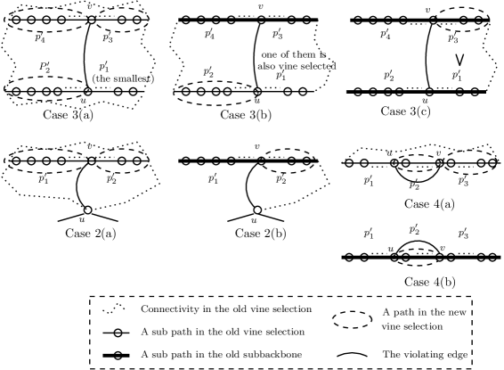
Figure 3: The different cases in Lemma 5.25. In case 2, the edge $e=uv$ is between a path and the backbone. In case 3, $e$ is between two different paths. In case 4, $e$ is inside the same path. The different sub-cases corresponds to the different possibilities of the paths to be either in the vine-selection, or as sub-backbones.

1. Both $u$ and $v$ are not on paths in $\mathcal{D}$ (they are in $S\cup B$). In this case $e$ is not a violating edge, which is impossible.

2. One of $u$ or $v$ is on a path in $\mathcal{D}$ and the other is not. In this case $|\mathcal{P}^{\prime}|=|\mathcal{P}|+1$. Assume $v\in p$, for some $p\in\mathcal{P}$, and $u\in S\cup B$, so $p=p^{\prime}_{1}\cup\{v\}\cup p^{\prime}_{2}$, where $p^{\prime}_{1},p^{\prime}_{2}\in\mathcal{P}^{\prime}$. As $|p|=n_{1}+n_{2}$ (since $|\cdot|$ is defined to be the number of vertices plus one), $\tilde{\Delta}=\log\frac{n_{1}n_{2}}{n_{1}+n_{2}}$.

   1. If $p\in A(\mathcal{D})$, then we construct $A(\mathcal{D}^{\prime})=A(\mathcal{D})\cup\{p^{\prime}_{1},p^{\prime}_{2}\}\setminus\{p\}$. $B(\mathcal{D}^{\prime})$ is connected, and $\Delta=\log\frac{n_{1}n_{2}}{n_{1}+n_{2}}$, so $\Delta\geq\tilde{\Delta}.$

   2. If $p\not\in A(\mathcal{D})$, then there is a simple path in $B(\mathcal{D})$ between $u$ and $v$. Without loss of generality, assume the path passes through $p^{\prime}_{2}$. Construct $A(\mathcal{D}^{\prime})=A(\mathcal{D})\cup\{p^{\prime}_{2}\}\setminus\{p\}$. $B(\mathcal{D}^{\prime})$ is connected, and $\Delta=\log n_{2}$, so $\Delta\geq\log n_{2}+\log\frac{n_{1}}{n_{1}+n_{2}}=\tilde{\Delta}.$

3. $u,v$ are on different paths, $u\in p$ and $v\in q$, for some $p,q\in\mathcal{P}$ and $p\neq q$. In this case $|\mathcal{P}^{\prime}|=|\mathcal{P}|+2$. Assume $p=p^{\prime}_{1}\cup\{u\}\cup p^{\prime}_{2}$ and $q=p^{\prime}_{3}\cup\{v\}\cup p^{\prime}_{4}$. Here $\tilde{\Delta}=\log\frac{n_{1}n_{2}n_{3}n_{4}}{(n_{1}+n_{2})(n_{3}+n_{4})}.$

   1. If $p,q\in A(\mathcal{D})$. Without loss of generality assume that $n_{1}=\min\{n_{1},n_{2},n_{3},n_{4}\}$. Construct $A(\mathcal{D}^{\prime})=A(\mathcal{D})\cup\{p^{\prime}_{2},p^{\prime}_{3},p^{\prime}_{4}\}\setminus\{p,q\}$. Obviously $B(\mathcal{D}^{\prime})$ is connected, and $\Delta=\log\frac{n_{2}n_{3}n_{4}}{(n_{1}+n_{2})(n_{3}+n_{4})}$. Without loss of generality, assume $n_{3}\leq n_{4}$, so $\log\frac{n_{2}n_{4}}{(n_{1}+n_{2})(n_{3}+n_{4})}\geq-2$. Thus

      $$\Delta=\log n_{3}+\log\frac{n_{2}n_{4}}{(n_{1}+n_{2})(n_{3}+n_{4})}\geq\log n_{3}-2\geq\tfrac{1}{2}\log n_{3}\geq\\ \tfrac{1}{4}(\log n_{3}+\log n_{1})\geq\tfrac{1}{4}\bigl{[}\log n_{3}+\log n_{1}+\log\frac{n_{2}n_{4}}{(n_{1}+n_{2})(n_{3}+n_{4})}\bigr{]}=\tfrac{1}{4}\tilde{\Delta}.$$

   2. If $p\in A(\mathcal{D})$, and $q\not\in A(\mathcal{D})$ (The case $q\in A(\mathcal{D})$ and $p\notin A(\mathcal{D})$ is similar). Without loss of generality, $n_{1}\leq n_{2}$. $p^{\prime}_{1}$ has two endpoints, one of which is adjacent to $u$. The other endpoint of $p^{\prime}_{1}$ is connected via a simple path in $B(\mathcal{D})$ to $v$. This path must contain either $p^{\prime}_{3}$ or $p^{\prime}_{4}$. Without loss of generality, assume it contains $p^{\prime}_{3}$. If $n_{1}\geq n_{3}$ then we construct $A(\mathcal{D}^{\prime})=A(\mathcal{D})\cup\{p^{\prime}_{1},p^{\prime}_{2}\}\setminus\{p\}$. If, on the other hand, $n_{1}<n_{3}$ then we construct $A(\mathcal{D}^{\prime})=A(\mathcal{D})\cup\{p^{\prime}_{3},p^{\prime}_{2}\}\setminus\{p\}$. In either case, $B(\mathcal{D}^{\prime})$ is connected, and

      $$\Delta=\log\frac{\max\{n_{1},n_{3}\}\cdot n_{2}}{n_{1}+n_{2}}=\log\max\{n_{1},n_{3}\}+\log\frac{n_{2}}{n_{1}+n_{2}}\geq\\ \tfrac{1}{2}\max\{\log n_{1},\log n_{3}\}\geq\tfrac{1}{4}(\log n_{1}+\log n_{3})\geq\tfrac{1}{4}(\log n_{1}+\log\min\{n_{3},n_{4}\})\geq\\ \tfrac{1}{4}\Bigl{[}\log n_{1}+\log\min\{n_{3},n_{4}\}+\log\frac{n_{2}\max\{n_{3},n_{4}\}}{(n_{1}+n_{2})(n_{3}+n_{4})}\Bigr{]}=\tfrac{1}{4}\tilde{\Delta}$$

   3. If $p,q\not\in A(\mathcal{D})$. Then there is a simple path in $B(\mathcal{D})$ from $u$ to $v$. Without loss of generality, assume it passes through $p^{\prime}_{1}$, and $p^{\prime}_{3}$. Without loss of generality, assume $n_{1}\leq n_{3}$. Construct $A(\mathcal{D}^{\prime})=A(\mathcal{D})\cup\{p^{\prime}_{3}\}$. $B(\mathcal{D}^{\prime})$ is connected, and

      $$\Delta=\log n_{3}\geq\frac{1}{2}\bigl{[}\log\min\{n_{1},n_{2}\}+\log\min\{n_{3},n_{4}\}\bigr{]}\geq\tfrac{1}{2}\tilde{\Delta}$$

4. $u,v$ are on the same path. In this case $|\mathcal{P}^{\prime}|=|\mathcal{P}|+2$. Assume $p=p^{\prime}_{1}\cup\{u\}\cup p^{\prime}_{2}\cup\{v\}\cup p^{\prime}_{3}$, for some $p\in\mathcal{P}$ and $p^{\prime}_{1},p^{\prime}_{2},p^{\prime}_{3}\in\mathcal{P}^{\prime}$. So $\tilde{\Delta}=\log\frac{n_{1}n_{2}n_{3}}{n_{1}+n_{2}+n_{3}}$. Here $e=uv$ does not contradict $\mathcal{D}$ being proper, implying that $n_{2}\geq(n_{1}+n_{2}+n_{3})^{1/4}$, so $\log n_{2}\geq\tfrac{1}{4}\log\max\{n_{1},n_{2},n_{3}\}$. Without loss of generality, assume that $n_{1}\leq n_{3}$.

   1. If $p\in A(\mathcal{D})$, then construct $A(\mathcal{D}^{\prime})=A(\mathcal{D})\cup\{p^{\prime}_{2},p^{\prime}_{3}\}\setminus\{p\}$.

      $$\Delta=\log\frac{n_{2}n_{3}}{n_{1}+n_{2}+n_{3}}=\log\min\{n_{2},n_{3}\}+\log\frac{\max\{n_{2},n_{3}\}}{n_{1}+n_{2}+n_{3}}\geq\\ \geq\log\min\{n_{2},n_{3}\}-\log 3\geq\tfrac{1}{2}\log\min\{n_{2},n_{3}\}\geq\\ \geq\tfrac{1}{10}(\log n_{1}+\log\min\{n_{2},n_{3}\})\geq\tfrac{1}{10}\tilde{\Delta}$$

   2. If $p\not\in A(\mathcal{D})$, then construct $A(\mathcal{D}^{\prime})=A(\mathcal{D})\cup\{p^{\prime}_{2}\}$.

      $$\Delta=\log n_{2}\geq\tfrac{1}{8}2\log\max\{n_{1},n_{2},n_{3}\}\geq\tfrac{1}{8}\tilde{\Delta}$$

∎

We combine lemmas 5.24 and 5.25:

Proof of Lemma 5.19.

We first find an initial decomposition (not necessarily proper) and a corresponding initial vine selection as required by Lemma 5.25. For a proper path, Lemma 5.24 gives the needed initial decomposition and vine selection. For a complex $(B,\mathcal{Q})$, we take $(\emptyset,\mathcal{Q})$ as the initial decomposition, and $\mathcal{Q}$ as the corresponding initial vine selection. Using Lemma 5.25 we obtain an irreducible decomposition and a corresponding vine selection. ∎

Proof of Lemma 5.20

We need the following definitions:

Definition 5.26.

Define a sequence $(c_{m})_{m\in\mathbb{N}}$ recursively as follows

$$c_{m}=\begin{cases}c/4&m<8^{4};\\ c_{\lceil m^{1/4}\rceil}\cdot\left(1-\frac{5}{m^{3/16}}\right)&\text{otherwise.}\end{cases}$$

We define a “good” vine decomposition $\mathcal{V}$ of a proper path $q$ related to a recursive decomposition $\mathcal{D}^{R}(q)$, to be a proper vine decomposition of $q$ such that

• For every path $p\in\mathcal{P}$, $|p|<|q|^{1/4}$.

• $\nu(\mathcal{V})\geq c_{|q|}\cdot\left[\tilde{v}(\mathcal{D}^{R}(q))-\log|q|\right]$.

Proposition 5.27.

There exists $c^{\prime}>0$ such that for all $m$, $c_{m}\geq c^{\prime}$.

Proof.

Define $c^{\prime}_{j}=\frac{c}{4}\prod_{i=2}^{j}(1-\frac{5}{8^{(4^{i})\cdot 3/16}})$, and $c^{\prime}=\lim_{j\rightarrow\infty}c^{\prime}_{j}$. It is easily seen that $(c_{m})_{m>0}$ and $(c^{\prime}_{j})_{j>0}$ are non-increasing and $c_{8^{4^{j}}}=c^{\prime}_{j}$. We have $c^{\prime}>0$, since $1>\frac{5}{8^{(4^{i})\cdot 3/16}}\geq 0$ and $\sum_{i=1}^{\infty}\frac{5}{8^{(4^{i})\cdot 3/16}}<\infty$. ∎

Thus, constructing a recursive irreducible decomposition along with “good” vine decomposition would suffice to prove Lemma 5.20. The following lemma is the inductive argument that allows the construction.

Lemma 5.28.

Let $\mathcal{D}^{R}(q)=(S,\{\mathcal{D}^{R}(p_{1}),\dots,\mathcal{D}^{R}(p_{s})\})$ be a recursive decomposition of a proper path $q$ such that $\mathcal{D}=(S,\{p_{1},\ldots,p_{s}\})$ is an irreducible decomposition. Assume that:

• There is a vine selection $A(\mathcal{D})$ of $\mathcal{D}$.

• For every sub-path $p_{i}$, there is a “good” vine decomposition $\mathcal{V}(p_{i})$ related to $\mathcal{D}^{R}(p_{i})$.

Then we can construct $\mathcal{V}$, a “good” vine decomposition related to $\mathcal{D}^{R}(q)$.

Proof.

Denote by $m_{i}=|p_{i}|$ and $M=|q|$. From the irreducibility property of $\mathcal{D}^{R}(q)$, $m_{i}\leq M^{{1}/{4}}$. For every $p\in A(\mathcal{D})$ we do the following:

• Let $m=|p|$. From the assumptions, the vines in $\mathcal{V}(p)=(B(p),\mathcal{P}(p))$ have lengths at most $m^{1/4}$. We partition $p$ to $t=\lceil m/(5m^{1/4})\rceil=\lceil m^{3/4}/5\rceil$ consecutive sub-paths $C_{1},\dots,C_{t}$, each of size between $(5-2)m^{1/4}$ and $(5+2)m^{1/4}$, such that no sub-path partitions a vine in $\mathcal{V}(p)$. Let $X_{i}$ be the sum of the values of the vines in $C_{i}$. Thus $\sum_{i}X_{i}=\nu(\mathcal{V}(p))$. Let $C=S_{i_{1}}$ be the sub-path that satisfies $X=X_{i_{1}}=\min_{i}\{X_{i}\}$, so $X\leq\frac{5}{m^{3/4}}\nu(\mathcal{V}(p))$. $S$ is partitioned into three consecutive sub-paths $C^{\text{lft}},C^{\text{mid}},C^{\text{rgt}}$ such that $|C^{\text{mid}}|=m^{1/4}$, and $|C^{\text{lft}}|\geq m^{1/4}$, $|C^{\text{rgt}}|\geq m^{1/4}$.

  Let $p^{\text{lft}}$, $p^{\text{rgt}}$ denotes the sub-paths $p$ that are to the left and to the right (respectively) of $C^{\text{mid}}$ in $p$. Let $B(p)$ denotes the backbone of $\mathcal{V}(p)$. We construct $\mathcal{V}^{\text{lft}}$, a vine decomposition of $p^{\text{lft}}$ by defining $B^{\text{lft}}$, the backbone of $\mathcal{V}^{\text{lft}}$, to be $B^{\text{lft}}=(B(p)\cup C^{\text{lft}})\cap p^{\text{lft}}$. We claim that $\mathcal{V}^{\text{lft}}$ is a legal vine decomposition, and that the endpoints of $p^{\text{lft}}$ are part of $B^{\text{lft}}$. It is easy to see that the endpoints of the vines in $\mathcal{V}^{\text{lft}}$ are adjacent to $B^{\text{lft}}$ and the endpoints of $p^{\text{lft}}$ are part of $B^{\text{lft}}$.

  We are left to prove that the sub-graph spanned by $B^{\text{lft}}$ is connected. First, note that $\exists v_{l}\in C^{\text{lft}}\cap B(p)$, otherwise $C^{\text{lft}}$ is part of a vine in $\mathcal{V}(p)$ and its length is at least $m^{1/4}$, which contradicts the assumptions. The sub-graph induced on $C^{\text{lft}}$ is obviously connected. For every vertex $u\in B^{\text{lft}}\setminus C^{\text{lft}}$, there is a path $r$ in $B(p)$ from $u$ to $v_{l}$. Consider the maximal prefix of $r$ which is entirely inside $p^{\text{lft}}$. The last vertex of the maximal prefix of $r$ must be inside $C^{\text{lft}}$, otherwise there is an edge $e$ in $p$ such that $|e|_{p}\geq|C^{\text{lft}}|=m^{1/4}$, in contradiction to the irreducibility property of $\mathcal{D}$. Thus $B^{\text{lft}}$ is connected.

  In conclusion, $\mathcal{V}^{\text{lft}}$ is a legal vine decomposition of $p^{\text{lft}}$. Similarly, we construct a vine decomposition $\mathcal{V}^{\text{rgt}}$ of $p^{\text{rgt}}$ such that the endpoints of $p^{\text{rgt}}$ are part of the backbone of $\mathcal{V}^{\text{rgt}}$.

We construct $\mathcal{V}$, a vine decomposition of $q$ such that every vertex in a sub-path $p\not\in A(\mathcal{D})$ will have the same role (part of the backbone or part of a vine) as in $\mathcal{V}(p)$. For $p\in A(\mathcal{D})$ we declare $C^{\text{mid}}(p)$ to be a vine, and the other vertices, to have the same role as in $\mathcal{V}^{\text{lft}}(p)$ and $\mathcal{V}^{\text{rgt}}(p)$. $\mathcal{V}$ is a vine decomposition of $q$ as it is seen from the previous discussion and because the endpoints of the sub paths are part of the backbone (see Def. 5.15). Also, every vine of $\mathcal{V}$ has length less than $M^{1/4}$.

Because $c_{m^{\prime}}$ is non-increasing as a function of $m^{\prime}$, $c_{M}=\min_{m^{\prime}\leq M^{1/4}}c_{m^{\prime}}(1-\frac{5}{m^{\prime}{}^{3/4}})$. Let $m=|p|$. From the construction, for every $p\in A(\mathcal{D})$,

$$\nu(\mathcal{V}^{\text{lft}}(p))+\nu(\mathcal{V}^{\text{rgt}}(p))\geq\left(1-\frac{5}{m^{3/4}}\right)\nu(\mathcal{V}(p))\geq\\ \geq\left(1-\frac{5}{m^{3/4}}\right)c_{m}\left(\tilde{v}(\mathcal{D}^{R}(p))-\log m\right)\geq c_{M}\left(\tilde{v}(\mathcal{D}^{R}(p))-\log m\right).$$

We conclude

$$\nu(\mathcal{V}) \geq\sum_{p\in A(\mathcal{D})}\tfrac{1}{4}\log|p|+\sum_{p\in A(\mathcal{D})}c_{M}\left[\tilde{v}(\mathcal{D}^{R}(p))-\log|p|\right]+$$

$$\quad+\sum_{p\not\in A(\mathcal{D})}\left[\tilde{v}(\mathcal{D}^{R}(p))-\log|p|\right]$$

$$\geq c_{M}\cdot\left[\sum_{i=1}^{s}\log|p_{i}|+\sum_{i=1}^{s}\left[\tilde{v}(\mathcal{D}^{R}(p_{i}))-\log|p_{i}|\right]\right]$$

$$=c_{M}\sum_{i=1}^{s}\tilde{v}(\mathcal{D}^{R}(p_{i}))=c_{M}\left[\tilde{v}(\mathcal{D}^{R}(q))-\log M\right].\qed$$

Proof of Lemma 5.20.

We show the existence of a recursive decomposition and “good” vine decomposition by induction on the structure of the recursive decomposition.

The base of the induction are simple paths whose inner vertices do not have other adjacent vertices. Such a path has a unique recursive decomposition, namely all the vertices are in the separating set of the decomposition. The “good” vine decomposition is also obvious: all the vertices are in the backbone.

Otherwise, we use Lemma 5.19 to get an irreducible decomposition $\mathcal{D}=(S,\mathcal{P})$ and a vine selection $A(\mathcal{D})$. Inductively, Each $p\in\mathcal{P}$ has a recursive decomposition $\mathcal{D}^{R}(p)$ along with a “good” vine decomposition $\mathcal{V}(p)$. Hence, all the assumptions of Lemma 5.28 are satisfied, and we get a recursive decomposition along with a “good” vine decomposition for the given proper path. ∎

Proof of Lemma 5.22

Proof of Lemma 5.22..

Assume that the first two cases in the statement of the Lemma do not hold. Denote $\mathcal{Q}=\{q_{1},\dots,q_{t}\}$. We divide the vertices of $q_{1}\cup\dots\cup q_{t}$ between four sets $X_{1}$, $X_{2}$, $X_{3}$ and $X_{4}$ as follows: Let $v_{1},v_{2},\dots,v_{m}$ be the vertices of $q_{1}\cup q_{2}\cup\dots\cup q_{t}$ ordered as the order in $q_{1},q_{2},\dots,q_{t}$. Let $t_{0}=1$ and $t_{4}=m$. For $i\in\{1,2,3\}$, let $t_{i}$ be the smallest index such that $t_{i}\geq t_{i-1}+h+1$ and $v_{t_{i}}$ is not on a path of $\mathcal{P}$. Now we assign $X_{i}=\{v_{t_{i-1}},\dots,v_{t_{i}}\}$. Note that the vertices $v_{t_{1}},v_{t_{2}},v_{t_{3}}$ might appear in two consecutive sets.

All four sets have at least $h$ unique vertices, unless there exists a path $p\in\mathcal{P}$ such that $|p|\geq h+1$. In this case we construct $\mathcal{V}^{\prime}$ from $\mathcal{V}$ by removing the path $p$. Here $\nu(\mathcal{V}^{\prime})=\nu(\mathcal{V})-\log|p|\geq\tfrac{23}{24}\nu(\mathcal{V}))$.

From here on, we assume all four sets has at least $h$ unique vertices. We denote by $\nu(X_{i})=\sum_{p}\log|p|$ where $p$ ranges over the paths in $\mathcal{P}$ contained in $X_{i}$. Thus $\sum_{i=1}^{4}\nu(X_{i})=\nu(\mathcal{V})$. Assume that $\nu(X_{i_{4}})=\max_{i\leq 4}\nu(X_{i})$, so $\nu(X_{i_{4}})\geq\nu(\mathcal{V})/4$.

For a vertex $u\in X_{i_{4}}\cap B_{2}$, define

$$C_{u}=\Bigl{\{}v\in(q_{1}\cup\cdots\cup q_{t})\setminus X_{i_{4}}:\ \begin{aligned} \exists r=\langle u,w_{1},\ldots,w_{s},v\rangle\text{ a path in }G^{s}\\ \text{ and }\{w_{1},\ldots,w_{s}\}\subseteq X_{i_{4}}\cap B_{2}\end{aligned}\Bigr{\}}.$$

Note that $C_{u}\neq\emptyset$. We say that $u\in X_{i_{4}}\cap B_{2}$ is locally connected to $A$ if $C_{u}\subseteq A$. Let $Y_{i_{j}}(j\leq 3)$ be the set of paths of $\mathcal{P}$ contained in $X_{i_{4}}$ having at least one of their endpoints locally connected to $X_{i_{j}}$. Then $\nu(Y_{i_{1}})+\nu(Y_{i_{2}})+\nu(Y_{i_{3}})\leq 2\nu(X_{i_{4}})$, since each path of $\mathcal{P}$ contained in $X_{i_{4}}$ is counted at most twice. Assume that $Y_{i_{1}}$ has the minimal value of the three, so $\nu(Y_{i_{1}})\leq\frac{2}{3}\nu(X_{i_{4}})$.

We remove from $\mathcal{V}$ all the unique vertices of $X_{i_{1}}$. Note that there are indeed enough vertices to remove since $X_{i_{1}}$ alone contains at least $h$ vertices that can be removed.

Next, We add to the backbone the following vertices: (i) The vertices of the vines in $Y_{i_{1}}$; and (iii) all the vertices in $X_{i_{2}}$ and $X_{i_{3}}$ to the backbone. The resulting is a “vine decomposition” $\tilde{\mathcal{V}}=(\tilde{B},\tilde{\mathcal{P}})$ that the endpoints of its vines are all part of its backbone, and $\nu(\tilde{\mathcal{V}})\geq\frac{1}{3}\nu(X_{i_{4}})\geq\frac{1}{12}\nu(\mathcal{V})$.

However, $\tilde{B}$ might be disconnected. It consists of at most 3 connected components: (i) One that contains $B_{1}$, (ii) one that contains $X_{i_{2}}$, and (iii) one that contains $X_{i_{3}}$. A more careful observation reveals that there might be at most 2 connected components: Assume $X_{i_{2}}$ is disconnected from $B_{1}$ in $\tilde{B}$. In this case $X_{i_{2}}$ is contained in one path $q_{i_{0}}\in\mathcal{Q}$. On one side of $X_{i_{2}}$ (in $q_{i_{0}}$), there are vertices from $X_{i_{1}}$, and in the other side, vertices from $X_{i_{4}}$. Now, either $X_{i_{3}}$ contains an endpoint of one of the paths of $\mathcal{Q}$ (in this case it is connected to $B_{1}$) or it is adjacent to $X_{i_{2}}$ in $q_{i_{0}}$ (in this case it is connected to $X_{i_{2}}$). In both cases we have only two connected components.

In case $\tilde{B}$ is disconnected we augment it as follows. Denote the connected components of $\tilde{B}$ by $C\supseteq X_{i_{2}}$ and $D\supseteq B_{1}$. On $q_{i_{0}}$, $X_{i_{4}}\cap q_{i_{0}}$ separates $X_{i_{2}}$ from $D\cap(q_{i_{0}}\cup\{q_{i_{0}}$’s neighbors in $B\})$.

Assume that $C$ is on the left side of $X_{i_{4}}\cap q_{i_{0}}$ in $q_{i_{0}}$. Let $u\in C\cap q_{i_{0}}$ be the right most vertex of $C$ in $q_{i_{0}}$. $u$ is either in $X_{i_{4}}$ or adjacent to $X_{i_{4}}$. Let $v\in D$ be the leftmost vertex of $D$ that is to the right of $u$ (in case no vertex of $q_{i_{0}}$ right of $u$ is in $D$, we take $v$ to be a vertex in $B_{1}$ adjacent to the rightmost vertex in $q_{i_{0}}$). The vertices of $q_{i_{0}}$ between $u$ and $v$ form a path $p\in\mathcal{P}$ which is also a vine in $\tilde{\mathcal{V}}$. We add them to the backbone of $\tilde{\mathcal{V}}$. The result is the desired vine decomposition $\mathcal{V}^{\prime}$, which has at least $h$ vertices less than $\mathcal{V}$, and

$$\nu(\mathcal{V}^{\prime})\geq\nu(\tilde{\mathcal{V}})-\log|p|\geq\tfrac{1}{12}\nu({\mathcal{V}})-\tfrac{1}{24}\nu({\mathcal{V}})\geq\nu(\mathcal{V})/24.$$

We observe that from the way $X_{i}$ were formed, for any path $q\in\mathcal{Q}$, $q\cap X_{i_{4}}$ is indeed a subpath, and one of its endpoints is adjacent to the backbone of $\mathcal{V}^{\prime}$. ∎

6 Refined Locality of Reference

Definition 6.1.

An extended access graph on a set of pages $\mathcal{P}$ is a finite labeled undirected graph $G=(V,E,\ell)$, with a labeling function $\ell:V\rightarrow{\cal P}$ that labels vertices with pages.

A request sequence $\sigma=(\ell(v_{i}))_{i\geq 1}$, is a finite sequence of labels attached to vertices from $G$, such that either $v_{i+1}=v_{i}$, or $v_{i}v_{i+1}\in E$. A paging algorithm should maintain the invariant, that following the $i$th request, $\ell(v_{i})$ should be in some page slot. The competitive measures $r_{\text{{On}}}(G,k)$, $r(G,k)$, $r_{\mathsf{obl}}(G,k)$ and their asymptotic counterparts are defined in a similar manner to the definitions for access graphs in Section 1.2.

For a given extended access graph $G$, we define a parameter $\Delta(G)$ that indicates “how quickly” the locality of reference may change $G$.

Definition 6.2.

$$\Delta(G)=\min\{s-1:\;\langle v_{1},v_{2},\dots,v_{s}\rangle\in\text{paths}(G),\ v_{1}\neq v_{s}\text{, and }\ell(v_{1})=\ell(v_{s})\}.$$

As convention, when $G$ is an (non extended) access graph, we fix $\Delta(G)=\infty$.

We remark that paging algorithms get only the names of the requested pages and not the names of the vertices. However for $\Delta(G)>2$ and assuming the starting vertex is known, online algorithms can easily reconstruct the sequence of the requested vertices from the sequence of the requested pages.

6.1 Truly Online Algorithms

Theorem 1 and Theorem 2 extend to the extended access graph model.

Theorem 3.

For any $\varepsilon>0$, and any extended access graph $G$ with $\Delta(G)>(1+\varepsilon)k$,

$$r_{\text{$\text{{Dto}}$}}(G,k) \leq\max\{O(r^{\infty}(G,k)),2/\varepsilon\}$$

$$r_{\text{$\text{{Rto}}$}}(G,k) \leq\max\{O(r^{\infty}_{\mathsf{obl}}(G,k)),2/\varepsilon\}.$$

In particular, for any fixed $\alpha>1$, Dto and Rto are very strongly competitive for any $G$ and $k$ satisfying $\Delta(G)>\alpha k$.

Proof.

Let $g$ denote the number of new pages in the current phase. We consider two cases: If $g\geq\varepsilon k$ then Dto and Rto fault at most $k\leq\frac{2}{\varepsilon}\cdot\frac{\varepsilon k}{2}\leq\frac{2}{\varepsilon}\cdot\frac{g}{2}$ times in the phase.

If, on the other hand, $g<\varepsilon k$, then during the current phase and the previous phase there were no requests to two different vertices with the same label, so the graph $G_{III}$ is an actual sub-graph of $G$. By the proofs of Theorem 2 and Theorem 1, Dto faults at most $O(g\cdot r^{\infty}(G,k))$ times and Rto faults at most $O(g\cdot r_{\mathsf{obl}}^{\infty}(G,k))$ times, in the phase. ∎

When $\Delta(G)$ is slightly greater than $k$, Dto and Rto do not work well, as is seen in the following example.

Example 6.3.

Consider the extended access graph $G=(V,E,\ell)$, where $V=\{1,2,\ldots,v_{k+1},v_{k+2}\}$, $E=\{v_{i}v_{i+1}:\;1\leq i\leq k+1\}$, and

$$\ell(v_{i})=\begin{cases}i&i\leq k+1\\ 1&i=k+2.\end{cases}$$

Here $\Delta(G)=k+1$. Consider the request sequence $\sigma=J_{1}J_{2}J_{3}\ldots$ where $J_{2i-1}=1,2,\ldots,k$ and $J_{2i}=k+1,1,k+1,k,\ldots,2$. Note that $(J_{i})_{i}$ is the phase partitioning of $\sigma$. Clearly, $r(G,k)=O(1)$. In contrast, Dto and Rto fault $\Omega(\log k)$ times [expected] during subphase III in each phase, and therefore $r^{\infty}_{\text{{Dto}}}(G,k)$ and $r^{\infty}_{\text{{Rto}}}(G,k)$ are $\Omega(\log k)$.

6.2 Very strongly competitive algorithm for paths with $k+1$ pages

In this section we present a very strongly competitive algorithm for graphs that are simple paths on $k+1$ pages. This algorithm will serve us in proving impossibility results concerning truly online algorithms.

Given a finite simple path $G=\langle v_{1},v_{2},\ldots,v_{m}\rangle$ with a surjective label function $\ell:\{v_{i}:\;1\leq i\leq m\}\rightarrow{\cal P}$, where $|{\cal P}|=k+1$. Fix a vertex $v_{i}$. We define a partial order $\prec_{i}$ on $\cal P$: $p\prec_{i}q$ if any path from $v_{i}$ to a vertex labeled by $q$ must include a vertex labeled by $p$. It is easy to verify that $\prec_{i}$ is indeed a partial order. Let $M_{i}$ be the set of maximal elements in $\prec_{i}$. Note that:

1. $M_{i}$ includes at most two pages that appear only on one side of $v_{i}$ in $G$.

2. Any request sequence that starts at $v_{i}$ and accesses all the pages in $M_{i}$, must access all the pages in $\cal P$.

We define linear orders on $M^{\prime}_{i}=\{p\in M_{i}:\;p$ appears on both sides of $v_{i}$ in $G\}$. For $p,q\in M^{\prime}_{i}$, $p\prec^{L}_{i}q$ if when going in $G$ from $v_{i}$ to the left, we reach a vertex labeled with $p$ before we reach a vertex labeled with $q$. Analogously, $p\prec^{R}_{i}q$ is defined to the right. Note that $p\prec_{i}^{R}q$ if and only if $q\prec_{i}^{L}p$.

Lemma 6.4.

$r^{\infty}_{\mathsf{obl}}(G,k)=\Omega(\max_{i}\log|M_{i}|)$.

Proof.

Let $i_{0}=\arg\max_{i}|M_{i}|$, so $|M_{i_{0}}|>0$. Using Yao’s Principle (cf. [3, Ch. 8]) we construct a probability distribution on the request sequences by the following iterative process: The request sequence is composed of periods, each period is composed of sub-periods. Let $N_{j}$ be the set of $\prec_{i_{0}}$–maximal pages that were left unmarked before the $j$th sub-period begins. At the beginning of a period $N_{1}=M_{i_{0}}$.

We describe the request sequence in the $j$th sub-period. The adversary begins from $v_{i_{0}}$. It chooses a page $p\in N_{j}$ such that $p$ is smaller than $|N_{j}|/2+1$ pages of $N_{j}$ under both $\prec^{L}_{i_{0}}$ and $\prec^{R}_{i_{0}}$ (its existence follows from a simple counting argument). If $p$ appears on both sides of $v_{i_{0}}$ in $G$, then the adversary chooses uniformly at random the left or the right side, otherwise he chooses the side on which $p$ appears. The adversary then requests the vertices in that direction until reaching the first vertex $v$ labeled with $p$, and then returns to $v_{i_{0}}$. At this point the $j$th sub-period ends. Note that $|N_{j+1}|\geq|N_{j}|/2-1$. The adversary continues this way until $N_{j}=\emptyset$, which means that all pages were requested during the period. At this point the period ends, and the adversary begins a new period.

During a period, an optimal off-line algorithm faults at most twice, because the request sequence consists of at most two phases.

Next we show that any online algorithm has $\Omega(\log|M_{i_{0}}|)$ expected number of faults of during a period.

To prove it we argue that there are $\Omega(\log|M_{i_{0}}|)$ sub-periods in a period and an online algorithm has an expected cost of at least half in each sub-period, except maybe two of them. There are at least $\Omega(\log|M_{i_{0}}|)$ sub-periods before $N_{j}$ becomes empty set, because in each sub-period the size of $N_{j}$ is roughly halved. In all sub-periods in which the target label $p$ appears on both sides of $v_{i_{0}}$, the expected number of faults of the online algorithm is at least $1/2$, since $\prec_{i_{0}}$-maximal pages that appear on both sides of $v_{i_{0}}$ must appear, at least on one side of $v_{i_{0}}$, after the hole. As all $\prec_{i_{0}}$-maximal pages appear on both sides of $v_{i_{0}}$, except maybe two, the claim follows. ∎

We shall see now a very strongly competitive deterministic marking online algorithm called Maxfar.

MAXFAR.

Maxfar is a marking algorithm. Assume the current phase began at $v_{i}$. On the $j$th fault in the phase, let $N_{j}\subset M_{i}$ be the set of unmarked $\prec_{i}$–maximal elements. Choose a page $p\in N_{j}$ in the middle of $N_{j}$ according to $\prec_{i}^{L}$ (which is also in the middle according to $\prec_{i}^{R}$) and evict it. If $N_{j}$ contains only pages that appear on only one side of $v_{i}$, evict one of them (there at most two such pages).

It is easy to see that $\{N_{j}\}_{j}$ is a decreasing sequence of sets, and $|N_{j+1}|\leq|N_{j}|/2+1$. Thus after at most $j=O(\log|M_{i_{0}}|)$ faults, $N_{j}=\emptyset$, and at this point, the phase is over. We conclude that $r_{\text{$\text{{Maxfar}}$}}(G,k)=O(\max_{i}\log|M_{i}|)$. Putting this together,

Theorem 4.

For any extended access graph $G$ which is a simple path on $k+1$ pages, $r_{\text{$\text{{Maxfar}}$}}(G,k)=O(r^{\infty}_{\mathsf{obl}}(G,k)).$

6.3 Impossibility Results

In this section we show that any truly online algorithm can not be very strongly competitive on extended access graphs, when $\Delta(G)$ is slightly less than $k$. Formally, we prove that

Theorem 5.

1. For any $0<f<k$, and any deterministic truly on-line paging algorithm $A$, there exists an extended access graph $G$ such that $\Delta(G)\geq k-f+1$ and $r_{A}(G,k)\geq f$ but $r(G,k)=O(\log k)$. In particular, for $f=f(k)=\omega(\log k)$, $r_{A}(G,k)=\omega(r(G,k))$.

2. For any $0<f<k$, and any randomized truly on-line paging algorithm $A$, there exists an extended access graph $G$ such that $\Delta(G)\geq k-f-1$ and $r_{A}(G,k)=\Omega(\log f)$, but $r_{\mathsf{obl}}(G,k)=O(\log k-\log f+\log\log f)$. In particular, for $f=f(k)=k^{1-o(1)}$, $r_{A}(G,k)=\omega(r_{\mathsf{obl}}(G,k))$.

Proof.

Fix $0<f^{\prime}=f+1<k$, and a truly online algorithm $A$.

Consider the following part of an extended access graph labeled with $k+1$ pages:

$$1,2,\ldots,k,k+1,x_{1},x_{2},\ldots,x_{f^{\prime}}.$$

The adversary maintains the invariant $\{x_{i}:\;1\leq i\leq f^{\prime}\}=\{1,\ldots,f^{\prime}\}$, but in some permutation that will be determined.

To prove part (1), assume $A$ is deterministic. We split the request sequence $\sigma$ into phases and show that each phase costs $A$ at least $f^{\prime}$, whereas it costs the adversary only $1$ (except the first phase, in which the cost for the adversary is $k$). We will also show that there exists an online algorithm that obtains a competitive ratio of $O(\log k)$ on this graph. By making the request sequence long enough (for $c$ phases where $c$ satisfies $k+(c-1)f^{\prime}\geq fc$), the first part of the theorem will be proved.

The adversary works in phases. Assume that in the previous phase the requested pages were $\{1,\dots,k\}$. Each phase is composed of $f^{\prime}$ sub-phases, indexed by $j$

For $j=0$, the adversary requests $x_{0}=k+1$. As $A$ is deterministic, the adversary knows what page has been evicted by $A$ to satisfy this request. Denote it by $p_{0}$. In general, in each subphase, the adversary requests a hole of $A$, and therefore to serve the request, $A$ must evict at least one page from its real memory. Denote a page evicted by $A$ in the $j$th sub-phase by $p_{j}$.

In the $j$th sub-phase the adversary does as follows: If $p_{j-1}>f^{\prime}$ then the adversary requests the pages $x_{j-1},x_{j-2},\ldots,x_{0}=k+1,k,\ldots,p_{j-1}+1,p_{j-1},p_{j-1}+1,p_{j-1}+2,\ldots,k,x_{0}=k+1,x_{1},\ldots,x_{j-1}.$ It then sets $x_{j}$ to be arbitrary page in $\{1,\ldots,f^{\prime}\}\setminus\{x_{1},\ldots,x_{j-1}\}$ and requests $x_{j}$. This is a legitimate traversal on the extended access graph.

If $p_{j-1}\leq f^{\prime}$ then: (i) If $p_{j-1}$ has not been requested yet in the current phase, then the adversary sets $x_{j}=p_{j-1}$, and requests it (ii) Otherwise there must be some $i\leq j$ such that $x_{i}=p_{j-1}$ and the adversary generates the requests $x_{j-1},x_{j-2},\ldots,x_{i},x_{i+1},\ldots,x_{j-1}$. It then sets $x_{j}$ to be arbitrary page in $\{1,\ldots,f^{\prime}\}\setminus\{x_{1},\ldots,x_{j-1}\}$ and requests $x_{j}$.

When $j=f^{\prime}$, the phase ends. $k$ different pages have been requested in this phase. $A$ had a fault in each sub-phase and therefore its cost has been at least $f^{\prime}$.

The above argument is for one phase, but we can continue this process for an additional $c$ phases, for any $c$, simply by adding an additional $c\cdot f^{\prime}$ vertices on the right hand side (right of $x_{f^{\prime}}$ above).

Note that (i) $\Delta(G)\geq k-f^{\prime}$ for any such graph; (ii) $G$ is a simple path on $k+1$ pages, so from Theorem 4, Maxfar has a competitive ratio of $O(\log k)$.

Next, we turn to prove an impossibility result for randomized truly online algorithms. The adversary constructs a graph similarly to the previous case, but now it does not know where the hole is. Instead it resorts to a random process as follows: It maintains a maximal unrequested sub-path $\langle i_{1},\dots,i_{2}\rangle$ of the vertices labeled $1,\dots,f^{\prime}$. In each sub-phase it first requests all the pages already requested during the phase. The adversary then sets $i_{3}=(i_{1}+i_{2})/2$, the midpoint vertex in the unrequested segment, and chooses uniformly at random one of the two:

• Requesting the pages $\{i_{3},\dots,i_{2}\}$ by setting $x_{j+1}=i_{2}$, $x_{j+2}=i_{2}-1$, $\dots,x_{j+(i_{2}-i_{3})+1}=i_{3}$, and then setting $j\leftarrow j+(i_{2}-i_{3})+1$.

• Requesting the pages $\{i_{1},\dots,i_{3}\}$ by setting $x_{j+1}=i_{3}$, $x_{j+2}=i_{3}-1$, $\dots,x_{j+(i_{3}-i_{1})+1}=i_{1}$, and then setting $j\leftarrow j+(i_{3}-i_{1})+1$.

After approximately $\log f^{\prime}$ sub-phases the phase ends. In each sub-phase, $A$ faults with probability at least $1/2$, and therefore the expected cost of $A$ in a phase is $\Omega(\log f)$.

Like the deterministic case, this process can be continued for an additional $c$ phases, for any $c$, simply by adding an additional vertices on the right hand side.

Note also that the construction maintains $\Delta(G)\geq k-f$, and that $G$ is a simple path on $k+1$ pages. Thus Maxfar is applicable in this scenario.

Assume $i\geq k+1$. To bound $M_{i}$, denote by $t$ the first time $v_{i}$ is reached by the adversary. Each sub-phase of the adversary after time $t$, contributes at most one maximal element to $\prec_{i}$, and thus, at most $\lceil\log f^{\prime}\rceil$ maximal elements are added to $M_{i}$ in each phase after time $t$. However, after $\lceil(k+1)/f^{\prime}\rceil$ phases since time $t$, all the pages also appear to the right of $v_{i}$, since each phase adds $f^{\prime}$ distinct pages to the right of $v_{i}$. Therefore $|M_{i}|\leq\left\lceil k/f^{\prime}\right\rceil\left\lceil\log f^{\prime}\right\rceil$. Note that a similar argument also holds for $i\leq k$. Thus, $r_{\text{{Maxfar}}}(G,k)=O(\log k-\log f^{\prime}+\log\log f^{\prime})$. ∎

7 Implementation

Storing $G_{0}$ requires only $O(k\log n)$ bits. We also need to keep track of:

1. The vertices requested so far in the current phase.

2. The current unevicted vertices of $G_{0}$.

3. $G_{0}$ for the next phase.

One way to construct $G_{0}$ for the next phase is to store a pointer from every page requested to the previously requested page. This pointer will be updated only once in a phase (the first time the page is accessed during the phase). The resulting data structure is a tree with pointers from the leaves upwards, and the root is the first page requested in the phase. At the end of a phase, the pointers are scanned and an image of $G_{0}$ is built in memory. This image contains vertices, pointers, and the virtual addresses associated with the vertices. In total (hardware registers and memory) the memory required is $O(k\log n)$ bits.

There is a rather efficient hardware implementation for processing page hits. The $\log n$ bit virtual address is translated to a $\log k$ page slot address (by the virtual address translation mechanism). The spanning tree is built on the $\log k$ bit address space of page slots but the virtual addresses ($\log n$ bits) are stored in the vertices. Hence, the hardware storage requirement for implementing page hits in Dto and Rto is one $\log k$ bits pointer and one extra bit (marking bit) associated with every page slot. The extra hardware processing associated with interpreting a page hit is one $\log k$ bits address comparison, one bit comparison, and (possibly) setting one $\log k$ bits pointer.

Dto and Rto, as presented here, use a spanning tree of $G_{P}$ as their reference access graph. It is easy to check that instead, we could have use any connected sub-graph of $G_{P}$. We can even use $G_{P}$ itself and store it using only $O(k\log n)$ bits (instead of the $O(k^{2}\log n)$ in the naive implementation). To do that, observe that there is no need to actually store edges whom both their endpoints have degree $\geq 3$. Thus, when a new edge is revealed we increase the degree of its endpoints, and “forget” all the edges in which both endpoints have degree $\geq 3$. In this way only $2k$ edges should be explicitly stored.

It would be of theoretical interest to reduce the memory requirements even further, to be independent of $n$. Our goal is to reduce the factor of $\log n$ in the storage requirement to $\log k$. Of course, the address translation table must still use $\Omega(k\log n)$ bits. But when we restrict ourselves to the paging eviction strategy, and assuming we are also told reliably whether a page request is a hit or a fault, we can allow small errors, if their total effect on the number of page faults is insignificant.

Consider a universal set of hash functions $h:\mathbb{N}\rightarrow\{0,\dots,m-1\}$, e.g., $h(x)=ax+b\pmod{m}$, where $m$ is prime and $a$ and $b$ are uniformly and independently sampled from $\mathbb{Z}_{m}$. We replace in Rto the usage of the virtual address of a page $p$ with the hash value of the page ($h(p)$).

In this case Rto may err and identify two different pages as the same. In the worst case, it would “confuse” Rto in the current and the next phase (because $G_{0}$ for the next phase is built incorrectly). Nonetheless, since Rto has the marking property, the damage is restricted to these two phases, and so such an error would add at most $2k$ page faults.

The probability that such a bad event happens is bounded from above by the following simple argument: consider the $\binom{k+g}{2}$ pairs of different pages requested during the last two phases. The probability that a pair of different pages collide is $1/m$, therefore the probability of an error occurring during a phase is at most $\binom{2k}{2}\frac{1}{m}=O\bigl{(}\frac{k^{2}}{m}\bigr{)}$. Choosing $m=\Theta(k^{3})$ insures that the expected number of added page faults due to collisions of hash values is $O(k\frac{k^{2}}{m})=O(1)$ per phase.

Hence, a data structure with $O(k\log m)=O(k\log k)$ bits gives a randomized algorithm with the same performance guarantees as the original Rto algorithm, up to a constant factor.

8 Concluding Remarks

In this paper we have studied the access graph model for locality of reference in paging. We have shown a somewhat surprising result: It is possible to be both truly online and still very strongly competitive in the access graph model. The resulting algorithms seems practical, and can be proven to work well even when the locality of reference changes.

The following issues are not resolved.

1. The proof of Lemma 4.2 is very lengthy. Is there a simpler and/or shorter proof?

2. In a preliminary version of this work [8] we claimed that both Dto and Rto can be patched so as to be very strongly competitive for any $G$ and $k$ as long as $\Delta(G)>k$. The patch we devised turned out to be erroneous. Still, we conjecture that very strongly competitive truly online algorithms are possible when $\Delta(G)>k$.

3. Finding an uniform and very strongly competitive algorithm for the extended access graph model.

4. Is there a very strongly competitive algorithm for the directed access graph model? Or is it computationally a hard problem?

Acknowledgement.

We would like to thank Yair Bartal, Nati Linial, and Gideon Stupp for helpful discussions.

References

- [1] L.A. Belady. A study of replacement algorithms for virtual storage computers. IBM Systems Journal, 5:78–101, 1966.
- [2] Shai Ben-David, Allan Borodin, Richard Karp, Gábar Tardos, and Avi Wigderson. On the power of randomization in on-line algorithms. Algorithmica, 11(1):2–14, January 1994.
- [3] Allan Borodin and Ran El-Yaniv. Online computation and competitive analysis. Cambridge University Press, Cambridge, UK, 1998.
- [4] Allan Borodin, Sandy Irani, Prabhakar Raghavan, and Baruch Schieber. Competitive paging with locality of reference. J. Comp. Syst. Sci., 50(2):244–258, April 1995.
- [5] Marek Chrobak and John Noga. LRU is better than FIFO. Algorithmica, 23:180–185, 1999.
- [6] Amos Fiat and Anna R. Karlin. Randomized and multipointer paging with locality of reference. In Proceedings of the 27th Annual ACM Symposium on Theory of Computing, pages 626–634, 1995.
- [7] Amos Fiat, Richard Karp, M. Luby, Lyle A. McGeoch, Daniel D. Sleator, and Neal E. Young. Competitive paging algorithms. Journal of Algorithms, 12:685–699, 1991.
- [8] Amos Fiat and Manor Mendel. Truly online paging with locality of reference (extended abstract). In Proceedings of the 38th Annual Symposium on Foundations of Computer Science, pages 326–335, 1997.
- [9] Amos Fiat and Ziv Rosen. Experimental studies of access graph based heuristics: Beating the lru standard? In 8th Annual ACM-SIAM Symposium on Discrete Algorithms, pages 63–72, 1997.
- [10] Sandy Irani, Anna R. Karlin, and Steven J. Phillips. Strongly competitive algorithms for paging with locality of reference. SIAM J. Comput., 25(3):477–497, June 1996.
- [11] Anna R. Karlin, Steven J. Phillips, and Prabhakar Raghavan. Markov paging. SIAM J. Comput., 30(3):906–922, 2000.
- [12] Daniel J. Kleitman and Douglass B. West. Spanning trees with many leaves. SIAM Journal on Discrete Mathematics, 4(1):99–106, 1991.
- [13] Carsten Lund, Steven Phillips, and Nick Reingold. Paging against a distribution and ip networking. J. Comp. Syst. Sci., 58(1):222–232, 1999.
- [14] Daniel D. Sleator and Robert E. Tarjan. Amortized efficiency of list update and paging rules. Communication of the ACM, 28:202–208, 1985.