Power Control for User Cooperation

Abstract

For a fading Gaussian multiple access channel with user cooperation, we obtain the optimal power allocation policies that maximize the rates achievable by block Markov superposition coding. The optimal policies result in a coding scheme that is simpler than the one for a general multiple access channel with generalized feedback. This simpler coding scheme also leads to the possibility of formulating an otherwise non-concave optimization problem as a concave one. Using the channel state information at the transmitters to adapt the powers, we demonstrate significant gains over the achievable rates for existing cooperative systems.

Index terms: Cooperative diversity, fading, multiple access channel, power control, user cooperation.

1 Introduction

Increasing demand for higher rates in wireless communication systems have recently triggered major research efforts to characterize the capacities of such systems. The wireless medium brings along its unique challenges such as fading and multiuser interference, which make the analysis of the communication systems more complicated. On the other hand, the same challenging properties of such systems are what give rise to the concepts such as diversity, over-heard information, etc., which can be carefully exploited to the advantage of the network capacity.

In the early 1980s, several problems which form a basis for the idea of user cooperation in wireless networks were solved. First, the case of a two user multiple access channel (MAC) where both users have access to the channel output was considered by Cover and Leung [1], and an achievable rate region was obtained for this channel. Willems and van der Meulen then demonstrated [2] that the same rate region is achievable if there is a feedback link to only one of the tansmitters from the channel output.

The capacity region of the MAC with partially cooperating encoders was obtained by Willems in [3]. In this setting, the encoders are assumed to be connected by finite capacity communication links, which allow the cooperation. Willems and van der Meulen also considered a limiting case of cooperation where the encoders “crib” from each other, that is, they learn each others’ codewords before the next transmission [4]. Several scenarios regarding which encoder(s) crib, and how much of the codewords the encoders learn, are treated and the capacity region for each case is obtained in [4]. The capacity of such channels are an upper bound to the rates achievable by cooperative schemes, since in the case of cribbing encoders, the sharing of information comes for free, i.e., the transmitters do not allocate any resources such as powers, to establish common information.

An achievable rate region for a MAC with generalized feedback was found in [5]. This channel model is worth special attention as far as the wireless channels are concerned, since it models the over-heard information by the transmitters. In particular, for a two user MAC with generalized feedback described by $({\cal X}_{1}\times{\cal X}_{2},P(y,y_{1},y_{2}|x_{1},x_{2}),{\cal Y}\times{\cal Y}_{1}\times{\cal Y}_{2})$, where user 1 has access to channel output $Y_{1}$ and user two has access to channel output $Y_{2}$, an achievable rate region is obtained by using a superposition block Markov encoding scheme, together with backward decoding, where the receiver waits to receive all $B$ blocks of codewords before decoding.

Recently, Sendonaris, Erkip and Aazhang have successfully employed the results of these rather general problems, particularly that of generalized feedback, to a Gaussian MAC in the presence of fading, leading to user cooperation diversity and higher rates [6]. In this setting, both the receiver and the transmitters receive noisy versions of the transmitted messages, and slightly modifying the basic relay channel case, the transmitters form their codewords not only based on their own information, but also on the information they have received from each other. It is assumed in [6] that channel state information for each link is known to the corresponding receiver on that link, and also phase of the channel state needs to be known at the transmitters in order to obtain a coherent combining gain. The achievable rate region is shown to improve significantly over the capacity region of the MAC with non-cooperating transmitters, especially when the channel between the two users is relatively good on average.

There has also been some recent work on user cooperation systems under various assumptions on the available channel state information, and the level of cooperation among the users. Laneman, Tse and Wornell [7] have characterized the outage probability behavior for a system where the users are allowed to cooperate only in half-duplex mode, and where no channel state information is available at the transmitters. For the relay channel, which is a special one-sided case of user cooperation, Host-Madsen and Zhang [8] have solved for power allocation policies that optimize some upper and lower bounds on the ergodic capacity when perfect channel state information is available at the transmitters and the receiver. For a user cooperation system with finite capacity cooperation links, Erkip [9] has proposed a suboptimal solution to the problem of maximizing the sum rate in the presence of full channel state information, where it was also noted that the resulting optimization problem is non-convex.

In this paper, we consider a two user fading cooperative Gaussian MAC with complete channel state information at the transmitters and the receiver, and average power constraints on the transmit powers. Note that, this requires only a small quantity of additional feedback, namely the amplitude information on the forward links, over the systems requiring coherent combining [6]. In this case, the transmitters can adapt their coding strategies as a function of the channel states, by adjusting their transmit powers [10, 11, 12]. We characterize the optimal power allocation policies which maximize the set of ergodic rates achievable by block Markov superposition coding. To this end, we first prove that the seemingly non-concave optimization problem of maximizing the achievable rates can be reduced to a concave problem, by noting that some of the transmit power levels are essentially zero at every channel state, which also reduces the dimensionality of the problem. By this, we also show that the block Markov superposition coding strategy proposed in [5] and employed in [6] for a Gaussian channel can be simplified considerably by making use of the channel state information. Due to the non-differentiable nature of the objective function, we use sub-gradient methods to obtain the optimal power distributions that maximize the achievable rates, and we provide the corresponding achievable rate regions for various fading distributions. We demonstrate that controlling the transmit powers in conjunction with user cooperation provides significant gains over the existing rate regions for cooperative systems.

2 System Model

We consider a two user fading Gaussian MAC, where both the receiver and the transmitters receive noisy versions of the transmitted messages, as illustrated in Figure 1. The system is modelled by,

$$Y_{0} =\sqrt{h_{10}}X_{1}+\sqrt{h_{20}}X_{2}+Z_{0}$$ (1)

$$Y_{1} =\sqrt{h_{21}}X_{2}+Z_{1}$$ (2)

$$Y_{2} =\sqrt{h_{12}}X_{1}+Z_{2}$$ (3)

where $X_{i}$ is the symbol transmitted by node $i$, $Y_{i}$ is the symbol received at node $i$, and the receiver is denoted by $i=0$; $Z_{i}$ is the zero-mean additive white Gaussian noise at node $i$, having variance $\sigma_{i}^{2}$, and $\sqrt{h_{ij}}$ are the random fading coefficients, the instantaneous realizations of which are assumed to be known by both the transmitters and the receiver. We assume that the channel variation is slow enough so that the fading parameters can be tracked accurately at the transmitters, yet fast enough to ensure that the long term ergodic properties of the channel are observed within the blocks of transmission [13].

The transmitters are capable of making decoding decisions based on the signals they receive and thus can form their transmitted codewords not only based on their own information, but also based on the information they have received from each other. This channel model is a special case of the MAC with generalized feedback [5]. The achievable rate region is obtained by using a superposition block Markov encoding scheme, together with backward decoding, where the receiver waits to receive all $B$ blocks of codewords before decoding. For the Gaussian case, the superposition block Markov encoding is realized as follows [6]: the transmitters allocate some of their powers to establish some common information in every block, and in the next block, they coherently combine part of their transmitted codewords. In the presence of channel state information, by suitably modifying the coding scheme given by [6] to accommodate for channel adaptive coding strategies, the encoding is performed by

$$X_{i}=\sqrt{p_{i0}(\mathbf{h})}X_{i0}+\sqrt{p_{ij}(\mathbf{h})}X_{ij}+\sqrt{p_{U_{i}}(\mathbf{h})}U_{i}$$ (4)

for $\quad i,j~{}\in~{}\{1,2\},\quad i\neq j$, where $X_{i0}$ carries the fresh information intended for the receiver, $X_{ij}$ carries the information intended for transmitter $j$ for cooperation in the next block, and $U_{i}$ is the common information sent by both transmitters for the resolution of the remaining uncertainty from the previous block, all chosen from unit-power Gaussian distributions. All the transmit power is therefore captured by the power levels associated with each component, i.e., $p_{i0}(\mathbf{h})$, $p_{ij}(\mathbf{h})$ and $p_{U_{i}}(\mathbf{h})$, which are required to satisfy the average power constraints,

$$E\left[p_{i0}(\mathbf{h})+p_{ij}(\mathbf{h})+p_{U_{i}}(\mathbf{h})\right]=E[p_{i}(\mathbf{h})]\leq\mbox{$\bar{p}$}_{i},\quad i=1,2.$$ (5)

Following the results in [6], it can be shown that the achievable rate region is given by the convex hull of all rate pairs satisfying

$$R_{1} < E\left[\log\left(1+\frac{h_{12}p_{12}(\mathbf{h})}{h_{12}p_{10}(\mathbf{h})+\sigma_{2}^{2}}\right)+\log\left(1+\frac{h_{10}p_{10}(\mathbf{h})}{\sigma_{0}^{2}}\right)\right]$$ (6)

$$R_{2} < E\left[\log\left(1+\frac{h_{21}p_{21}(\mathbf{h})}{h_{21}p_{20}(\mathbf{h})+\sigma_{1}^{2}}\right)+\log\left(1+\frac{h_{20}p_{20}(\mathbf{h})}{\sigma_{0}^{2}}\right)\right]$$ (7)

$$R_{1}+R_{2} < \min\left\{E\left[\log\left(1+\frac{h_{10}p_{1}(\mathbf{h})+h_{20}p_{2}(\mathbf{h})+2\sqrt{h_{10}h_{20}p_{U_{1}}(\mathbf{h})p_{U_{2}}(\mathbf{h})}}{\sigma_{0}^{2}}\right)\right],\right.$$ (8)

$$\left.\qquad\;\;E\left[\log\left(1+\frac{h_{12}p_{12}(\mathbf{h})}{h_{12}p_{10}(\mathbf{h})+\sigma_{2}^{2}}\right)+\log\left(1+\frac{h_{21}p_{21}(\mathbf{h})}{h_{21}p_{20}(\mathbf{h})+\sigma_{1}^{2}}\right)\right]\right.$$

$$\left.\qquad\;\;+E\left[\log\left(1+\frac{h_{10}p_{10}(\mathbf{h})+h_{20}p_{20}(\mathbf{h})}{\sigma_{0}^{2}}\right)\right]\vphantom{\log\left(1+\frac{h_{10}p_{1}(\mathbf{h})+h_{20}p_{2}(\mathbf{h})+2\sqrt{h_{10}h_{20}p_{U_{1}}(\mathbf{h})p_{U_{2}}(\mathbf{h})}}{\sigma_{0}^{2}}\right)}\right\}$$

where the convex hull is taken over all power allocation policies that satisfy (5).

For a given power allocation, the rate region in (6)-(8) is either a pentagon or a triangle, since, unlike the traditional MAC, the sum rate constraint in (8) may dominate the individual rate constraints completely. The achievable rate region may alternatively be represented as the convex hull of the union of all such regions. Our goal is to find the power allocation policies that maximize the rate tuples on the rate region boundary.

3 Structure of the Sum Rate and the Optimal Policies

We first consider the problem of optimizing the sum rate of the system, as it will also shed some light onto the optimization of an arbitrary point on the rate region boundary. The sum rate (8) is not a concave function of the vector of variables $\mathbf{p}(\mathbf{h})=[p_{10}(\mathbf{h})~{}p_{12}(\mathbf{h})~{}p_{U_{1}}(\mathbf{h})~{}p_{20}(\mathbf{h})\\ ~{}p_{21}(\mathbf{h})~{}p_{U_{2}}(\mathbf{h})]$, due to the existence of variables in the denominators. In what follows, we show that for the sum rate to be maximized, for every given $\mathbf{h}$, at least two of the four components of $[p_{10}(\mathbf{h})~{}p_{12}(\mathbf{h})~{}p_{20}(\mathbf{h})~{}p_{21}(\mathbf{h})]$ should be equal to zero, which reduces the dimensionality of the problem and yields a concave optimization problem.

Proposition 1

Let the effective channel gains normalized by the noise powers be defined as $s_{ij}=h_{ij}/\sigma_{j}^{2}$. Then, for the power control policy $\mathbf{p}^{*}(\mathbf{h})$ that maximizes (8), we need

1. $p_{10}^{*}(\mathbf{h})=p_{20}^{*}(\mathbf{h})=0$, if $s_{12}>s_{10}$ and $s_{21}>s_{20}$

2. $p_{10}^{*}(\mathbf{h})=p_{21}^{*}(\mathbf{h})=0$, if $s_{12}>s_{10}$ and $s_{21}\leq s_{20}$

3. $p_{12}^{*}(\mathbf{h})=p_{20}^{*}(\mathbf{h})=0$, if $s_{12}\leq s_{10}$ and $s_{21}>s_{20}$

$\left.\begin{tabular}[h]{lll}4.&$p_{12}^{*}(\mathbf{h})=p_{21}^{*}(\mathbf{h})=0$\\ &\qquad\quad{\footnotesize OR}\\ &$p_{10}^{*}(\mathbf{h})=p_{21}^{*}(\mathbf{h})=0$\\ &\qquad\quad{\footnotesize OR}\\ &$p_{12}^{*}(\mathbf{h})=p_{20}^{*}(\mathbf{h})=0$\end{tabular}\right\}\mbox{if}\;s_{12}\leq s_{10}\;\mbox{and}\;s_{21}\leq s_{20}$

Proof:  To simplify the notation, let us drop the dependence of the powers on the channel states, whenever such dependence is obvious from the context. Let $p_{i}=p_{i0}+p_{ij}+p_{U_{i}}$ be the total power allocated to a given channel state. Let us define

$$A =1+s_{10}p_{1}+s_{20}p_{2}+2\sqrt{s_{10}s_{20}p_{U_{1}}p_{U_{2}}}$$ (9)

$$B =\frac{1+s_{10}p_{10}+s_{20}p_{20}}{(1+s_{12}p_{10})(1+s_{21}p_{20})}$$ (10)

$$C =\left(1+s_{12}(p_{10}+p_{12})\right)\left(1+s_{21}(p_{20}+p_{21})\right)$$ (11)

Then, an equivalent representation of the sum rate in (8) is

$$R_{\mbox{\footnotesize sum}}=\min\left\{E\left[\log(A)\right],E\left[\log(BC)\right]\right\}$$ (12)

Now, let us arbitrarily fix the total power level, $p_{i}$, as well as the power level used for cooperation signals, $p_{U_{i}}\leq p_{i}$, allocated to a given state for each user. For each such allocation, the quantities $A$ and $C$ appearing in the sum rate expression are fixed, i.e., allocating the remaining available power $p_{i}-p_{U_{i}}$ among $p_{i0}$ and $p_{ij}$ will not alter these quantities. Note that, such allocation also does not alter the total power consumption at the given state, so we may limit our attention to the maximization,

$$\max_{\{p_{10},p_{20}\}} \;\;B\left(p_{10},p_{20}\right)$$

s.t. $$\;\;p_{10}+p_{12}=p_{1}-p_{U_{1}}$$

$$\;\;p_{20}+p_{21}=p_{2}-p_{U_{2}}$$ (13)

The partial derivatives of $B$ with respect to $p_{10}$ and $p_{20}$ are

$$\frac{\partial B}{\partial p_{10}}=\frac{s_{10}-s_{12}(1+s_{20}p_{20})}{(1+s_{12}p_{10})^{2}(1+s_{21}p_{20})}$$ (14)

$$\frac{\partial B}{\partial p_{20}}=\frac{s_{20}-s_{21}(1+s_{10}p_{10})}{(1+s_{21}p_{20})^{2}(1+s_{12}p_{10})}$$ (15)

Therefore, we make the following conclusions:

1. $s_{12}>s_{10}$, $s_{21}>s_{20}$. Then, $\frac{\partial B}{\partial p_{10}}<0$ and $\frac{\partial B}{\partial p_{20}}<0$, i.e., $B(p_{10},p_{20})$ is monotonically decreasing in both $p_{10}$ and $p_{20}$, therefore the sum rate is maximized at $p_{10}=p_{20}=0$.

2. $s_{12}>s_{10}$, $s_{21}\leq s_{20}$. Then, $\frac{\partial B}{\partial p_{10}}<0$, and the function is maximized at $p_{10}=0$ for any $p_{20}$. But this gives $\frac{\partial B}{\partial p_{20}}|_{p_{10}=0}>0$, meaning $p_{20}$ should take its maximum possible value, i.e., $p_{21}=0$.

3. $s_{12}\leq s_{10}$, $s_{21}>s_{20}$. Follows the same lines of case 2 with roles of users 1 and 2 reversed.

4. $s_{12}\leq s_{10}$, $s_{21}\leq s_{20}$. In this case, the partial derivatives of $B$ can be both made equal to zero within the constraint set, yielding a critical point. However, using higher order tests, it is possible to show that this solution corresponds to a saddle point, and $B$ is again maximized at one of the boundaries, $p_{10}=0$, $p_{20}=0$, $p_{10}=p_{1}-p_{U_{1}}$, $p_{20}=p_{2}-p_{U_{2}}$. Inspection of the gradient on these boundary points yields one of the three corner points $\{(p_{1}-p_{U_{1}},0),(0,p_{2}-p_{U_{2}}),(p_{1}-p_{U_{1}},p_{2}-p_{U_{2}})\}$ as candidates, each of which corresponds to one of the solutions in case 4.

   Although two of the components of the power vector are guaranteed to be equal to zero, which ones will be zero depends on the $p_{i}$ and $p_{U_{i}}$ that we fixed, therefore we are not able to completely specify the solution, independent of $p_{i}$ and $p_{U_{i}}$, in this case. On the other hand, the settings of interest to us are those where the channels between the cooperating users are on average much better than their direct links, since it is in these settings when cooperative diversity yields high capacity gains [6]. In such scenarios, the probability of both users’ direct link gains exceeding their corresponding cooperation link gains (case 4) is a very low probability event. Therefore, which of the three possible operating points is chosen is not of practical importance, and we can safely fix the power allocation policy to one of them to carry on with our optimization problem for the other variables. Although admittedly this argument is likely to cause some suboptimality in our scheme, as will be seen in the numerical examples, we still obtain a significant gain in the achievable rates.

 $\Box$

The significance of this result is two-fold. Firstly, given a channel state, it greatly simplifies the well known block Markov coding, in a very intuitive way: if the direct links of both users are inferior to their cooperation links, the users do not transmit direct messages to the receiver as a part of their codewords, and they use each other as relays. If one of the users’ direct channel is better than its cooperation channel, and the other user is in the opposite situation, then the user with the strong direct channel chooses to transmit directly to the receiver, while the weaker direct channel user still chooses to relay its information over its partner. Second important implication of this result is that it now makes the problem of solving for the optimal power allocation policy more tractable, since it simplifies the constraint set on the variables, and more importantly, this makes the sum rate a concave function over the reduced set of constraints and variables.

Corollary 1

The sum rate $R_{\mbox{\footnotesize sum}}$ given by (8), (12) is a concave function of $\mathbf{p}(\mathbf{h})$, over the reduced constraint set described by Proposition 1.

Proof:  The proof of this result follows from directly substituting the zero power components into the sum rate expression in (12). Note that in each of the four cases, the second function in the minimization, i.e., $\log(BC)$ takes either the form $\log(1+a)+\log(1+b)$, or $\log(1+a+b)$, both of which are clearly jointly concave in $a$ and $b$. Also, $\log(A)$ is clearly a concave function of $\mathbf{p}(\mathbf{h})$ since it is a composition of a concave function with the concave and increasing logarithm. The desired result is obtained by noting that the minimum of two concave functions is concave.  $\Box$

Thus far we have discussed the structure of the sum rate, as well as some properties of the optimal power allocation that maximizes that rate. We now turn back to the problem of maximizing other rate points on the rate region boundary. To this end, we point out another remarkable property of the solution in Proposition 1. Consider maximizing the bound on $R_{1}$ in (6). For fixed $p_{U_{1}}$ and $p_{1}$, it is easy to verify that all of the available power should be allocated to the channel with the higher gain, i.e., if $s_{12}>s_{10}$, then we need $p_{10}=0$ and $p_{12}=p_{1}-p_{U_{1}}$. The same result also applies to $R_{2}$. But this shows that, the policies described in Proposition 1 completely agree with optimal policies for maximizing the individual rate constraints in cases 1-3, and they also agree if we choose the operating point in case 4 to be $p_{12}=0,\;p_{21}=0$. Therefore, the allocation in Proposition 1 enlarges the entire rate region in all directions (except for the subtlety in case 4 for the sum rate). This has the benefit that the weighted sum of rates, say $R_{\bm{\mu}}=\mu_{1}R_{1}+\mu_{2}R_{2}$ also has the same concavity properties of the sum rate, since for $\mu_{i}>\mu_{j}$, the weighted sum of rates can be written as $R_{\bm{\mu}}=\mu_{j}R_{\mbox{\footnotesize sum}}+(\mu_{i}-\mu_{j})R_{i}$, where both $R_{\mbox{\footnotesize sum}}$ and $R_{i}$ are concave. Optimum power control policies that achieve the points on the boundary of the achievable rate region can then be obtained by maximizing the weighted sum of rates, which is the goal of the next section.

4 Rate Maximization via Subgradient Methods

In this section we focus on maximizing the weighted sum of rates. To illustrate both the results of the preceding section and the problem statement for this section more precisely, let us consider, without loss of generality, the case when $\mu_{1}\geq\mu_{2}$, and write down the optimization problem explicitly:

$$\max_{\mathbf{p}(\mathbf{h})}\; (\mu_{1}-\mu_{2})\left\{\vphantom{\int}E_{1,2}\left[\log(1+p_{12}(\mathbf{h})s_{12})\right]\right.$$

$$+\left.\vphantom{\int}E_{3,4}\left[\log(1+p_{10}(\mathbf{h})s_{10})\right]\right\}+\mu_{2}\min\left\{\vphantom{\int}E[\log(A)],\right.$$

$$+E_{1}\left[\log(1+p_{12}(\mathbf{h})s_{12})+\log(1+p_{21}(\mathbf{h})s_{21})\right]$$

$$+E_{2}\left[\log(1+p_{12}(\mathbf{h})s_{12})+\log(1+p_{20}(\mathbf{h})s_{20})\right]$$

$$+E_{3}\left[\log(1+p_{10}(\mathbf{h})s_{10})+\log(1+p_{21}(\mathbf{h})s_{21})\right]$$

$$+\left.E_{4}\left[\log(1+p_{10}(\mathbf{h})s_{10}+p_{20}(\mathbf{h})s_{20})\right]\vphantom{\int}\right\}$$

s.t. $$E_{3,4}\left[p_{10}(\mathbf{h})\right]+E_{1,2}\left[p_{12}(\mathbf{h})\right]+E\left[p_{U_{1}}(\mathbf{h})\right]\leq\mbox{$\bar{p}$}_{1}$$

$$E_{2,4}\left[p_{20}(\mathbf{h})\right]+E_{1,3}\left[p_{21}(\mathbf{h})\right]+E\left[p_{U_{2}}(\mathbf{h})\right]\leq\mbox{$\bar{p}$}_{2}$$ (16)

where, $E_{S}$ denotes the expectation over the event that case $S\subset\{1,2,3,4\}$ from Proposition 1 occurs, and $A$ is as given by (9). Note that the objective function is concave, and the constraint set is convex, therefore we conclude that any local optimum for the constrained optimization problem is a global optimum. Although $R_{\bm{\mu}}$ is differentiable almost everywhere since it is concave, its optimal value is attained along the discontinuity of its gradient, namely when the two arguments of the min operation are equal. Hence, we solve the optimization problem using the method of subgradients from non-differentiable optimization theory [14, 15].

The subgradient methods are very similar to gradient ascent methods in that whenever the function is differentiable (in our case almost everywhere), the subgradient is equal to the gradient. However, their major difference from gradient ascent methods is that they are not necessarily monotonically non-decreasing. Let us denote the objective function in (4) by $R_{\bm{\mu}}$. A subgradient for the concave function $R_{\bm{\mu}}(\mathbf{p})$ is any vector $\mathbf{g}$ that satisfies [15],

$$R_{\bm{\mu}}(\mathbf{p}^{\prime})\leq R_{\bm{\mu}}(\mathbf{p})+(\mathbf{p}^{\prime}-\mathbf{p})^{\top}\mathbf{g}$$ (17)

and the subgradient method for the constrained maximization uses the update [15]

$$\mathbf{p}(k+1)=[\mathbf{p}(k)+\alpha_{k}\mathbf{g}_{k}]^{{\dagger}}$$ (18)

where $[\cdot]^{{\dagger}}$ denotes the Euclidean projection onto the constraint set, and $\alpha_{k}$ is the step size at iteration $k$. There are various ways to choose $\alpha_{k}$ to guarantee convergence to the global optimum; for our particular problem, we choose the diminishing stepsize, normalized by the norm of the subgradient to ensure the convergence [14]

$$\alpha_{k}=\frac{a}{b+\sqrt{k}}\frac{1}{\parallel\mathbf{g}\parallel}$$ (19)

While the subgradient method is a powerful tool to obtain the global optimum of (4), it does not shed light onto the characteristics of the optimal power allocation policies. Although it is in general difficult, if not impossible, to state the optimal policy in a closed form, we provide a simplified case as an example, and provide conditions the optimal policies should satisfy, in the next subsection.

4.1 Properties of the Optimal Power Allocation: An Example

Throughout the analysis in this subsection, we assume for simplicity of the derivations that the fading distributions are such that all realizations of the fading values satisfy $s_{12}>s_{10}$ and $s_{21}>s_{20}$, i.e., the system always operates in the more interesting case 1. This particular case is of practical interest since the cooperating transmitters are likely to be closely located with less number of scatterers and obstructions when compared to their paths to the receiver, and thus have better channel conditions among each other. We also consider maximizing the sum capacity, i.e., $\mu_{1}=\mu_{2}$. Under these assumptions, since $p_{10}(\mathbf{h})=p_{20}(\mathbf{h})=0$ always, the problem of maximizing the sum rate, given in (8) and also obtained from (4) by inserting $\mu_{1}=\mu_{2}$, reduces to

$$\max_{\mathbf{p}(\mathbf{h})}\;\; \min\left\{E\left[\log(D)\right],E\left[\log\left(1+s_{12}p_{12}(\mathbf{h})\right)+\log\left(1+s_{21}p_{21}(\mathbf{h})\right)\right]\right\}$$

s.t. $$E\left[p_{12}(\mathbf{h})+p_{U_{1}}(\mathbf{h})\right]\leq\mbox{$\bar{p}$}_{1}$$

$$E\left[p_{21}(\mathbf{h})+p_{U_{2}}(\mathbf{h})\right]\leq\mbox{$\bar{p}$}_{2}$$

$$p_{12}(\mathbf{h}),p_{U_{1}}(\mathbf{h}),p_{21}(\mathbf{h}),p_{U_{2}}(\mathbf{h})\geq 0,\quad\forall\mathbf{h}$$ (20)

where

$$D=1+s_{10}\left(p_{12}(\mathbf{h})+p_{U_{1}}(\mathbf{h})\right)+s_{20}\left(p_{21}(\mathbf{h})+p_{U_{2}}(\mathbf{h})\right)+2\sqrt{s_{10}s_{20}p_{U_{1}}(\mathbf{h})p_{U_{2}}(\mathbf{h})}$$ (21)

Note that, the maximum of the objective function is attained only when the arguments of the $\min$ operation are equal, or else it would be possible to increase the smaller argument while decreasing the larger, just by transferring the transmit power between the cooperation signals $p_{U_{i}}(\mathbf{h})$ and $p_{ij}(\mathbf{h})$ at some $\mathbf{h}$, while keeping their sum constant, and therefore not violating the average power constraints. Hence, to overcome the difficulties arising from the non-differentiability of the cost function, the $\min$ in the cost function can be replaced by an equality constraint in the constraint set, and the problem can be restated with a new differentiable objective function as

$$\max_{\mathbf{p}(\mathbf{h})}\;\; E\left[\log\left(1+s_{12}p_{12}(\mathbf{h})\right)+\log\left(1+s_{21}p_{21}(\mathbf{h})\right)\right]$$ (22)

s.t. $$E\left[\log(D)\right]=E\left[\log\left(1+s_{12}p_{12}(\mathbf{h})\right)+\log\left(1+s_{21}p_{21}(\mathbf{h})\right)\right]$$ (23)

$$E\left[p_{12}(\mathbf{h})+p_{U_{1}}(\mathbf{h})\right]\leq\mbox{$\bar{p}$}_{1}$$ (24)

$$E\left[p_{21}(\mathbf{h})+p_{U_{2}}(\mathbf{h})\right]\leq\mbox{$\bar{p}$}_{2}$$ (25)

$$p_{12}(\mathbf{h}),p_{U_{1}}(\mathbf{h}),p_{21}(\mathbf{h}),p_{U_{2}}(\mathbf{h})\geq 0,\quad\forall\mathbf{h}$$ (26)

Associating the Lagrange multiplier $\gamma$ to the equality constraint (23), $\lambda_{1},\lambda_{2}>0$ to the power constraints (24),(25), and $\xi_{i}(\mathbf{h})\geq 0$, $i=1,\cdots,4$ to the non-negativity constraints (26), and noting that the power constraints need to be satisfied by equality, we obtain the Karush-Kuhn-Tucker (KKT) necessary conditions for optimality. Note that for optimality, for any given $\mathbf{h}$, the components $p_{U_{1}}(\mathbf{h})$ and $p_{U_{2}}(\mathbf{h})$ should be either both positive or both zero. Therefore, it is sufficient to analyze these two cases.

First let $p_{U_{1}}(\mathbf{h}),p_{U_{2}}(\mathbf{h})>0$. Then, the KKT conditions reduce to

$$(1+\gamma)\frac{s_{12}}{1+s_{12}p_{12}(\mathbf{h})} \leq\lambda_{1}+\gamma\frac{s_{10}}{D}$$ (27)

$$(1+\gamma)\frac{s_{21}}{1+s_{21}p_{21}(\mathbf{h})} \leq\lambda_{2}+\gamma\frac{s_{20}}{D}$$ (28)

$$\gamma\frac{\sqrt{s_{10}s_{20}p_{U_{2}}(\mathbf{h})}+s_{10}\sqrt{p_{U_{1}}(\mathbf{h})}}{D\sqrt{p_{U_{1}}(\mathbf{h})}} =-\lambda_{1}$$ (29)

$$\gamma\frac{\sqrt{s_{10}s_{20}p_{U_{1}}(\mathbf{h})}+s_{20}\sqrt{p_{U_{2}}(\mathbf{h})}}{D\sqrt{p_{U_{2}}(\mathbf{h})}} =-\lambda_{2}$$ (30)

From (29) and (30), it follows that there is a linear relationship between the optimal $p_{U_{1}}(\mathbf{h})$ and $p_{U_{2}}(\mathbf{h})$, i.e.,

$$\lambda_{1}^{2}s_{20}p_{U_{1}}(\mathbf{h})=\lambda_{2}^{2}s_{10}p_{U_{2}}(\mathbf{h})$$ (31)

Next, we include the case when $p_{U_{1}}(\mathbf{h})=p_{U_{2}}(\mathbf{h})=0$ in our analysis. The partial derivatives $\frac{\partial D}{\partial p_{U_{i}}(\mathbf{h})}$, $i=1,2$ are not well defined when $p_{U_{i}}(\mathbf{h})$ are both zero. However, the above derivation shows that the optimal solution is guaranteed to lie on the line given by (31), since $(p_{U_{1}}(\mathbf{h}),p_{U_{2}}(\mathbf{h}))=(0,0)$ also lies on the same line. Therefore, it is sufficient to evaluate the optimality conditions along the line (31) for $p_{U_{1}}(\mathbf{h})=p_{U_{2}}(\mathbf{h})=0$, as well as for $p_{U_{1}}(\mathbf{h}),p_{U_{2}}(\mathbf{h})>0$. Substituting (29) into (27), (30) into (28), using (31), and extending (29) and (30) to include the case $p_{U_{1}}(\mathbf{h}),p_{U_{2}}(\mathbf{h})=(0,0)$, we obtain the overall set of necessary conditions for the optimality of the power allocation policy as,

$$\frac{s_{12}}{1+s_{12}p_{12}(\mathbf{h})} \leq\frac{1}{(1+\gamma)}\frac{\lambda_{1}^{2}s_{20}}{\lambda_{2}s_{10}+\lambda_{1}s_{20}} \mbox{w.e. if}\;p_{12}(\mathbf{h})>0$$ (32)

$$\frac{s_{21}}{1+s_{21}p_{21}(\mathbf{h})} \leq\frac{1}{(1+\gamma)}\frac{\lambda_{2}^{2}s_{10}}{\lambda_{2}s_{10}+\lambda_{1}s_{20}} \mbox{w.e. if}\;p_{21}(\mathbf{h})>0$$ (33)

$$-\lambda_{1} \leq\frac{\gamma}{D}\left(s_{10}+\frac{\lambda_{1}}{\lambda_{2}}s_{20}\right) \mbox{w.e. if}\;p_{U_{1}}(\mathbf{h})>0$$ (34)

$$-\lambda_{2} \leq\frac{\gamma}{D}\left(s_{20}+\frac{\lambda_{2}}{\lambda_{1}}s_{10}\right) \mbox{w.e. if}\;p_{U_{2}}(\mathbf{h})>0$$ (35)

where w.e. stands for “with equality.”

These conditions shed some light onto the structure of the optimal power allocation policy: when the channel gains $s_{10},s_{20}$ from the transmitters to the receiver are fixed, the optimal power levels associated with the components intended for the other transmitter, $p_{12}(\mathbf{h})$ and $p_{21}(\mathbf{h})$, are independent of each other and are obtained by single user waterfilling over the individual link gains $s_{12}$ and $s_{21}$, respectively. The direct link gains $s_{10}$ and $s_{20}$ determine the water level. This is easily observed by denoting the right hand sides of (32) and (33) by the constants $\nu_{1}$ and $\nu_{2}$ (since $s_{10}$ and $s_{20}$ are fixed), and solving for $p_{12}(\mathbf{h})$ and $p_{21}(\mathbf{h})$, keeping in mind the equalities are satisfied only when the power levels are positive, i.e.,

$$p_{12}(\mathbf{h})=\left(\frac{1}{\nu_{1}}-\frac{1}{s_{12}}\right)^{+}$$ (36)

$$p_{21}(\mathbf{h})=\left(\frac{1}{\nu_{2}}-\frac{1}{s_{21}}\right)^{+}$$ (37)

where $(\cdot)^{+}$ denotes $\max(0,\cdot)$.

Once $p_{12}(\mathbf{h})$ and $p_{21}(\mathbf{h})$ are calculated, they can be substituted into (34) and (35) with $D$ defined as in (21) to obtain $p_{U_{i}}$. On the other hand, the computation of the optimal power levels require solving for the Lagrange multipliers $\lambda_{i}$ and $\gamma$ that satisfy the power constraints, which would require a multi-dimensional search. Moreover, due to the constraint (28) being potentially non-convex for some power values, the solution to the KKT conditions may not be sufficient to guarantee optimality. In the next section, we obtain the optimal power allocation policy numerically using the subgradient method, and then demonstrate by simulations that the optimal power allocation policy possesses the properties described in this subsection.

5 Simulation Results

In this section we provide some numerical examples to illustrate the performance of the proposed joint power allocation and cooperation scheme.

Figure 2 illustrates the achievable rate region we obtain for a system with $\mbox{$\bar{p}$}_{i}=\sigma_{i}^{2}=1$, subject to uniform fading, where the links from the transmitters to the receiver are symmetric and take values from the set $\{0.025,0.050,\cdots,0.25\}$, each with probability $1/10$, while the link among the transmitters is also symmetric and uniform, and takes the values $\{0.26,0.27,\cdots,0.35\}$. Notice that here, we have intentionally chosen the fading coefficients such that the cooperation link is always better than the direct links, therefore, the system operates only in case 1 of Proposition 1. Consequently, in this particular case, our power allocation scheme is actually the optimal power allocation policy for the block Markov superposition encoding scheme.

The region for joint power control and cooperation is generated using the subgradient method with parameters $a=50$ and $b=5$. We carried out the optimization for various values of the priorities $\mu_{i}$ of the users, each of which give a point on the rate region boundary, and then we performed a convex hull operation over these points. We observe that power control [10, 11, 12] by itself improves on the rate region of the cooperative system with no power control, for rate pairs close to the sum rate, by utilizing the direct link more efficiently. Joint user cooperation and power control scheme significantly improves on all other schemes, as it takes advantage of both cooperation diversity and time diversity in the system. In fact, we can view this joint diversity utilization as adaptively performing coding, medium accessing and routing, thereby yielding a cross-layer approach for the design of the wireless communication system.

Figure 3 also corresponds to a system with unit SNR, but this time subject to Rayleigh fading, i.e., the power gains to the receivers are exponential random variables, with $E[h_{10}]=E[h_{20}]=0.3$, $E[h_{12}]=E[h_{21}]=0.6$. In this setting, all four cases in Proposition 1 are realized, and there is potentially some loss over the optimally achievable rates. However, we obtain a very similar set of rate regions to the uniform case, indicating that in fact the loss, if any, is very small thanks to the very low probability of both of the direct links outperforming the cooperation link.

It is interesting to note in both Figures 2 and 3, cooperation with power control improves relatively less over power control only near the sum capacity. This can be attributed to the fact that, for the traditional MAC, the sum rate is achieved by time division among the users, which does not allow for coherent combining gain [11]. Therefore, it is not surprising to see that in order to attain cooperative diversity gain, users may have to sacrifice some of the gain they obtain from exploiting the time diversity.

In Figure 4, we illustrate the convergence of the subgradient method. The objective function is $R_{\bm{\mu}}$ with $\mu_{1}=2$ and $\mu_{2}=1$, and the step size parameters are varied. We observe that, by choosing larger step sizes, the non-monotonic behavior of the subgradient algorithm becomes more apparent, however the convergence is significantly faster than the smaller step sizes, as the algorithm is more likely to get near the optimal value of the function in the initial iterations. Note that, in our simulations we terminated the algorithm after $1000$ iterations, and the three curves would eventually converge after sufficiently large number of iterations.

Figures 5(a) and 5(b) demonstrate the waterfilling nature of the optimal power levels $p_{12}(\mathbf{h})$, and $p_{21}(\mathbf{h})$, as obtained in Section 4.1. These power levels correspond to the sum rate point on Figure 2, and were obtained by using the subgradient algorithm, after 1000 iterations. The direct link gains are fixed to the values $s_{10}=0.2$ and $s_{20}=0.15$. As dictated by (32) and (33), the “water level” for $p_{12}$ is higher, and the threshold channel state level to start transmitting is lower. We see that after 1000 iterations, the subgradient approach nearly satisfies the optimality conditions.

6 Conclusions

We have addressed the problem of optimal power allocation for a fading cooperative MAC, where the transmitters and the receiver have channel state information, and are therefore able to adapt their coding and decoding strategies by allocating their resources. We have characterized the power control policies that maximize the rates achievable by block Markov superposition coding, and proved that, in the presence of channel state information, the coding strategy is significantly simplified: given any channel state, for each of the users, among the three signal components, i.e., those that are intended for the receiver, for the other transmitter, and for cooperation, at least one of the first two should be allocated zero power at that channel state. This result also enabled us to formulate the otherwise non-concave problem of maximizing the achievable rates as a concave maximization problem. The power control policies, which are jointly optimal with block Markov coding, were then obtained using subgradient method for non-differentiable optimization. The resulting achievable rate regions for joint power control and cooperation improve significantly on cooperative systems without power control, since our joint approach makes use of both cooperative diversity and time diversity.

Figure 1: Two user fading cooperative MAC.

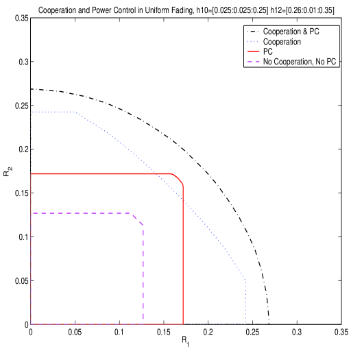
Figure 2: Rates achievable by joint power control and user cooperation for uniform fading.

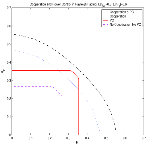
Figure 3: Rates achievable by joint power control and user cooperation for Rayleigh fading.

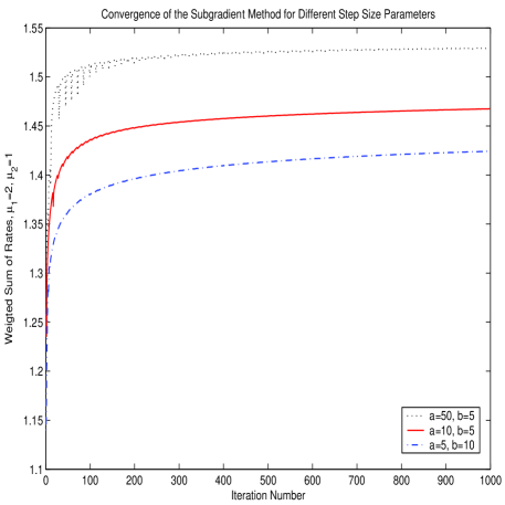
Figure 4: Convergence of $R_{\bm{\mu}}$ using subgradient method for different step size parameters.

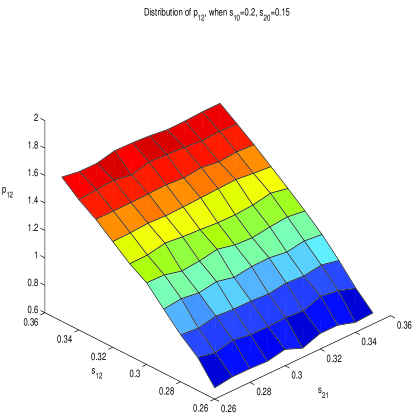
(a) The power level $p_{12}(\mathbf{h})$ as a function of $s_{12}$ and $s_{21}$.

(b) The power level $p_{21}(\mathbf{h})$ as a function of $s_{12}$ and $s_{21}$.

Figure 5: Power distributions obtained using the projected subgradient method.

References

- [1] T. M. Cover and C. S. K. Leung. An Achievable Rate Region for the Multiple Access Channel with Feedback. IEEE Trans. on Information Theory, 27(3):292-298, May 1981.
- [2] F. M. J. Willems and E. C. van der Meulen. Partial Feedback for the Discrete Memoryless Multiple Access Channel. IEEE Trans. on Information Theory, 29(2):287-290, March 1983.
- [3] F. M. J. Willems. The Discrete Memoryless Multiple Access Channel with Partially Cooperating Encoders. IEEE Trans. on Information Theory, 29(3):441-445, May 1983.
- [4] F. M. J. Willems and E. C. van der Meulen. The Discrete Memoryless Multiple Access Channel with Cribbing Encoders IEEE Trans. on Information Theory, 31(3):313-327, May 1985.
- [5] F. M. J. Willems, E. C. van der Meulen and J. P. M. Schalkwijk. An Achievable Rate Region for the Multiple Access Channel with Generalized Feedback. In Proc. Allerton Conference, Monticello, IL, October 1983.
- [6] A. Sendonaris, E. Erkip and B. Aazhang. User Cooperation Diversity – Part I: System Description. IEEE Trans. on Communications, 51(11): 1927–1938, November 2003.
- [7] J. N. Laneman, D. N. C. Tse and G. W. Wornell. Cooperative Diversity in Wireless Networks: Efficient Protocols and Outage Behavior. IEEE Trans. on Information Theory, 50(12): 3062–3080, December 2004.
- [8] A. Host-Madsen and J. Zhang. Capacity Bounds and Power Allocation for Wireless Relay Channels. IEEE Trans. on Information Theory, 51(6):(2020–2040), June 2005.
- [9] E. Erkip. Capacity and Power Control for Spatial Diversity. In Proc. Conference on Information Sciences and Systems, pp. WA4-28/WA4-31, Princeton, NJ, March 2000.
- [10] A. J. Goldsmith and P. P. Varaiya. Capacity of Fading Channels with Channel Side Information. IEEE Trans. on Information Theory, 43(6):1986–1992, November 1997.
- [11] R. Knopp and P. A. Humblet. Information Capacity and Power Control in Single-cell Multiuser Communications. In Proc. IEEE ICC, June 1995.
- [12] S. Hanly and D.N.C. Tse. Multiaccess Fading Channels – Part I: Polymatroid Structure, Optimal Resource Allocation and Throughput Capacities. IEEE Trans. on Information Theory, 44(7):2796–2815, November 1998.
- [13] E. Biglieri, J. Proakis and S. Shamai (Shitz). Fading Channels: Information-theoretic and Communications Aspects. IEEE Trans. on Information Theory, 44(6):2619–2692, October 1998.
- [14] N. Z. Shor. Minimization Methods for Non-Differentiable Functions. Springer-Verlag, 1979.
- [15] D. P. Bertsekas. Nonlinear Programming. Athena Scientific, 1995.