University of Iowa Department of Computer Science Technical Report TR-01-06
Localization in Wireless Sensor Grids

Abstract

This work reports experiences on using radio ranging to position sensors in a grid topology. The implementation is simple, efficient, and could be practically distributed. The paper describes an implementation and experimental result based on RSSI distance estimation. Novel techniques such as fuzzy membership functions and table lookup are used to obtain more accurate result and simplify the computation. An 86% accuracy is achieved in the experiment in spite of inaccurate RSSI distance estimates with errors up to 60%.

1 Introduction

Sensor networks fundamentally depend on location information for applications, which must bind spatial coordinates with sensed data. In addition, location can be useful for routing, power management, and other services. A localization (or positioning) service enables sensor nodes to acquire their spatial coordinates without having to program and deploy each sensor to a precise location.

In some cases position can be obtained by having Global Positioning System (GPS) on each sensor node, however this can have high expense, power cost, and put problematic constraints on deployment. Instead of using GPS, most self-localization algorithms assume only some sensor nodes can obtain their position information directly, and they are called anchors or beacons (by contrast, some algorithms construct relative coordinates only, and may use constraint solving techniques to combine local maps [14]). Using anchor positions, positions of other sensor nodes will then be calculated. Already there is extensive literature on the general problem of localization in wireless sensor networks, with solutions ranging from specialized ranging assumptions to complex algorithms that minimize overall positioning error [12, 15, 19, 21, 10, 4, 23, 25, 2, 13, 8, 9, 18].

The general problem of (self-) localization makes few assumptions about the topology of the network beyond basic communication connectivity and density (both sensor and anchor) constraints: the topology can be arbitrary and sensor deployment could be some random process. Presently, sensors are often expensive enough to justify more careful deployment than a random one; an economical emplacement of sensors for uniform coverage is a regular tiling [5] or grid topology. In [3], a large-scale wireless sensor grid is implemented and evaluated. Some localization schemes [22], [23] are also based on the grid deployment. The question driving our investigation is: does the assumption of a grid topology reduce the localization problem to a simple, practically implementable one? In a wireless sensor grid, one has more position constraint information than in a randomly placed network. With this additional information, we hope for a fast localization algorithm with small memory footprint, that could reasonably be run on the current generation of sensor nodes.

Contribution. In this paper, we investigate a very simple approach to localization for wireless sensor networks in a grid topology. The algorithm consumes little computing power and does not depend on high precision in distance estimation. It can be implemented in a distributed manner at different levels. Despite its almost naïve approach to assigning grid positions based on table lookup from hop distance and despite significant radio ranging errors, we find reasonable results (the reader may look ahead to Figure 4 for illustrative results). Our experimental results were obtained in rough and grassy terrain using RSSI for ranging, where acoustic ranging — the foundation for other distributed localization research [14] — has been difficult to use [10].

The rest of the paper is organized as follows. Section 2 describes the grid topology and anchor placement. Section 3 introduces a table lookup algorithm for localization and discusses different implementation possibilities. Section 4 presents experimental results and compares our algorithm to related results. Section 5 provides analysis of the algorithm, and Section 6 contains conclusions and future work.

2 Preliminaries

2.1 Grid Topology and Anchor Placement

We assume a grid topology with a rectangular perimeter; the grid can be divided into segments such that each segment has its own set of anchors. In our initial implementation, each segment has a basestation to run the localization algorithm. We discuss later how this assumption could be removed to get a fully distributed implementation with no basestation. The output of localization is an assignment of sensor nodes to the grid positions.

The size of each segment will affect the number of anchor nodes in the whole network and the performance of the algorithm. When each segment contains fewer nodes, and still has same number of anchors, then more anchors are needed for the whole grid. But the localization will be faster in this case and have better accuracy.

We field-tested our algorithm in a 5 by 10 grid segment. Figure 1 shows the topology, where the $(x,y)$ position of some points is shown. This topology is similar to the segment topology suggested in [3], which put vertices of the grid in a roughly hexagonal pattern. In this layout, the unit length of $y$-axis is twice the unit length of $x$-axis. This guarantees that each grid edge (that is, the line between nearest points) is of length at most 2: as explained in [3], this design gives each sensor sufficiently many communication neighbors to achieve desired redundancy for multi-hop routing, while efficiently providing sensor coverage of the entire field.

In our test, the segment has four anchors in the segment at grid positions (12,0), (3,1), (17,3), and (8,4). Anchors need to be placed carefully to ensure sufficient accuracy in localization. We provide some constraints on anchor placement in section 3, however the general problems of optimizing the number of anchors and optimizing anchor placement remain open.

The error in deployment for our experiment is discussed in section 4.

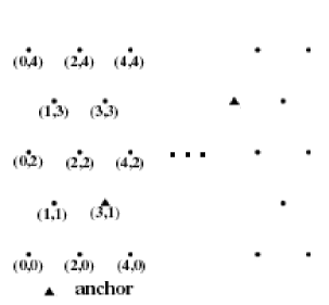
Figure 1: segment topology

2.2 Grid Distance

In our algorithm, we will use the number of grid hops on the shortest path between two nodes to represent the distance between them. The advantage of this representation is that it reduces the complexity of computing in localization (for instance, no floating-point calculation is needed). For two grid positions, it is also easy to find the formula calculating distance between them. For two positions (a,b) and (c,d), the distance between them is given by

$$\textit{dist}[\,(a,b),\;(c,d)\,]\quad=\quad\max\left(\frac{(|a-c|+|b-d)}{2},|b-d|\right)$$ (1)

3 Localization Algorithm and Implementation

Our localization algorithm is a simple algorithm using table lookup. The entire procedure has three stages. The first stage is to calculate a table, where each grid position has an entry. The entry for a grid position $p$ is a 4-tuple, consisting of grid distances between $p$ and four anchors. At least three anchors are necessary for localization; we found four anchors to be an improvement over three anchors, and the scheme can easily be generalized to a larger number of anchors. The second stage establishes the one-hop neighborhood for each sensor node, and for each node $q$, calculates a 4-tuple, consisting of grid distances between $q$ and the anchors using the one-hop neighborhood information. The third stage performs the table lookup and then refines the result of the lookup. Our algorithm is shown in Figure  2.

	stage 1:
	calculate grid distance table for the grid
		positions
	stage 2:
	each node $p$ sends a group of 30 messages
	each node forwards all the RSSI readings to
		the base station
	for each sender $p$, base station calculates
		a score for all receivers
	decide one-hop neighborhood for all nodes
	stage3:
	calculate distance between each node $q$
		and the anchors
	for each node $q$,look up in the table for
		a match
	for each unoccupied position, find the
		most likely node
	send out the assignments

Figure 2: localization algorithm

The implementation of this algorithm in one segment can be either centralized or distributed. We will describe the centralized implementation first. Also each stage of this algorithm can be implemented differently. For example, in the second stage, different ranging techniques can be used to help establishing the one-hop neighborhood.

3.1 Table Establishment and Anchors

Using formula (1), defined in Section 2, it is simple to calculate the distances from any grid position $p$ to the anchors; therefore when the grid is designed or deployed the table can be calculated and disseminated as needed for the subsequent stages.

In order for table lookup to be unambiguous, no pair of tuples in the table should be identical (otherwise two different grid points could have the same lookup). This constrains anchor placement. If anchors are placed in a line, then there will be much symmetry in the segment and different positions have identical tuples, which should be avoided. In our experiment, we set up the segment same as in [3], we found that if the 4 anchors form a parallelogram, then no table entries are identical. We have simulated different parallelogram placements in one segment, and found when the anchors are placed close to the segment border, the performance is slightly better. Similar observations can be found in other localization schemes [20].

3.2 One-hop Neighborhood using RSSI

We use Received Signal Strength Indicator(RSSI) for distance estimation in our implementation to obtain, for each node, an estimate of its one-hop neighborhood. Simplifying this task was our design of the grid, which defined the one-hop distance between neighbors to be about nine meters. We assume that the deployment error for each node is within a defined tolerance (see Section 4).

The RSSI ranging works as follows. A sensor node sends out a radio message with a certain signal strength and one field of this message records the signal strength of sending. The receiver of this message can measure the signal strength of the received message. Given a model of how signal strength reduces with distance (in our case obtained empirically), the original signal strength and received signal strength can be compared and the distance between the sender and receiver can be estimated. The advantage of RSSI ranging is that it is very simple and needs no additional hardware and little computing power. The disadvantage of RSSI ranging is that the accuracy is poor[1]; radio strength can be affected by the environment, the relative angles of emplacement for a pair of sensors, and manufacturing variances in radio devices.

For RSSI ranging in our implementation, we used a group of messages to deal with variation (we did not use advanced filters in our experiments, preferring to use the simplest of techniques). In our experiments, we notice that even with group size of 30, over the same distance, the mean RSSI reading varies considerably, as has been previously observed for similar hardware [24]. Put another way, the mean received signal strength readings can be same over different distances. To reduce the inaccuracy of RSSI ranging and get better one-hop neighborhood information, instead of having estimation of the real distance between a single pair of sender and receiver, we forward statistics of the RSSI readings to the base station.

Experience of other researchers [24, 17, 26] suggests that no elementary model may exist for how signal strength behaves as a function of distance. Therefore, instead of trying to find an analytical model for RSSI, we used a machine learning approach in our investigation. Machine learning for RSSI-based localization was previously used in [7], where Bayesian networks were trained.

We use fuzzy membership functions [6] to calculate a score for each receiver by looking at average RSSI reading, number of received messages, maximum and minimal RSSI readings, and the rank of RSSI readings among all receivers. For each property, we assign one fuzzy membership function. According to the classification in [6], we choose the membership functions based on reliability concerns with respect to the particular problem. From our implementation, even the very simple function forms (linear and triangular functions) are sufficient for this part. Finally we decide the one-hop neighborhood for the sender by checking the scores of the receivers. The score is in fact another fuzzy membership function. For this function, we use Distance Approach, one of the semantic approaches in fuzzy membership function design. This approach concentrates more on practical meaning and interpretation of membership. It is ideal for multi-attribute decision making [11]. This approach considers requirements on different attributes. It will assign operations for fuzzy logic. For instance, let $f_{A}$ and $f_{B}$ be fuzzy membership functions for attributes $A$ and $B$; then fuzzy membership function for “$A$ and $B$” is $min(f_{A},f_{B})$, and for “very $A$” is $f_{A}^{2}$. So we can interpret empirical rules such as “if very $A$ and $B$, then $C$ is likely” into functions.

After choosing the forms of the fuzzy membership functions, we need to decide the parameters for these functions. We conducted extensive tests for calibration. We performed tests with different spacing between nodes, relative angles, weather and terrain conditions. From the training data we collected from the tests, we determined the parameters to best distinguish 1-hop neighbors from more distant neighbors. In Section 5, we will show how well these functions work.

We give an example here on how to choose parameters for fuzzy membership functions. The fuzzy membership function $f_{avg}$ for an average RSSI reading $x$ to be “numerically like” a 1-hop reading is a combination of 3 simple linear functions.

$$f_{avg}(x)=\left\{\begin{array}[]{ll}1&x<a\\ \frac{b-x}{b-a}&a\leq x<b\\ 0&x\geq b\end{array}\right.$$

In our tests, generally, if the distance is smaller, the reading is smaller. So a smaller reading implies a more likely 1-hop reading. Thus we chose the function in this form.

Here, $a$ and $b$ are parameters of this fuzzy membership function. We need to determine these two parameters from our data. We want to choose them to be thresholds that only a small part of 2-hop readings are smaller than $a$ and most of the 1-hop readings are smaller than $b$. So We chose the $10^{th}$ percentile of average readings over 2-hop distances for $a$, and the $95^{th}$ percentile of average readings over 1-hop distances for $b$.

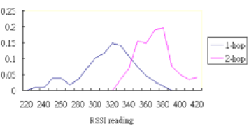
Figure 3: distribution for 1-hop and 2-hop readings

Figure 3 shows the distributions of 1-hop and 2-hop readings. So for our training data, $a=343$, and $b=361$.

An advantage of using machine learning with fuzzy membership function is that we do not have strong assumption for the underlying distribution of the RSSI reading over a certain distance.

An observation from the experiment is that by running a $\chi^{2}$ goodness-of-fit test on these two distributions, we found that the reading distributions for a fixed distance might not always be normal distribution, as assumed in [14, 16]. For 2-hop readings, it is not statistically significant to reject the hypothesis that the distribution is normal. But for 1-hop readings, the test yields $\chi^{2}=30.11$, for $p=0.01$, the $\chi^{2}$ for degree of freedom of 15 is 30.58, so with high significance, we can reject the hypothesis that the distribution of 1-hop readings is normal.

Similar to $f_{avg}$, we have fuzzy membership function $f_{rel}$, which describes how much an average RSSI reading $x$ is “relatively like” a 1-hop reading by checking all average RSSI readings for the same sender. Let $s$ denote the sender of the messages, and $R_{s}$ denote the set of nodes which report an average RSSI reading for $s$. If $|R_{s}|<2$, $f_{rel}$ is always 1. When $|R_{s}|$ is at least 2, let $max_{s}$ denote the mean of the 2 strongest average RSSI readings reported by $R_{s}$.

$$f_{rel}(x)=\left\{\begin{array}[]{ll}1&x<1.05max_{s}\\ 1-\frac{x-1.05max_{s}}{0.1max_{s}}&1.05max_{s}\leq x<1.15max_{s}\\ 0&x\geq 1.15max_{s}\end{array}\right.$$

If a receiver receives most of the messages in the message group from a sender, the average RSSI reading is more reliable than that from just a few messages. Meanwhile, from the training data we collected, we observe that 1-hop neighbors generally receive more messages than the 2-hop neighbors. Also with reduced power of radio signals and a message rate of 10 messages/s, we have not observed obvious message collisions, so it is not necessary to schedule the messages.

Function $f_{num}$ is used to determine whether an average RSSI reading $x$ is “like in volume” to a 1-hop reading by checking the number of messages on which $x$ is based. Let $x_{num}$ denote this number, $s$ denote the sender of the messages, and $most_{s}$ denote the most number of messages from $s$ that are received by a receiver.

$$f_{num}(x)=\left\{\begin{array}[]{ll}0&x_{num}<0.65most_{s}\\ \frac{x-0.65most_{s}}{0.25most_{s}}&0.65most_{s}\leq x_{num}<0.9most_{s}\\ 1&x_{num}\geq 0.9most_{s}\end{array}\right.$$

After calculating the fuzzy membership functions for different attributes, we use a fuzzy rule to get a score for the sender/receiver pair. From the training data we collected, we chose the rule for judging whether an average reading of a sender/receiver pair is like a 1-hop reading to be, it is “numerically like”, or, “relatively like” and very “like in volume”. So the score is calculated by the following.

$$score(x)=max(f_{avg}(x),min(f_{rel}(x),f_{num}^{2}(x)))$$

3.3 Table Look-up and Refinement

After establishing the one-hop neighborhood for every sensor node, the algorithm constructs shortest paths for each node to all the anchors in the segment. Thus it has a 4-tuple for each sensor node $q$, consisting of grid distances between $q$ and the anchors. Next, a table lookup is attempted: if it matches a table entry of unoccupied position $p$, then the algorithm assigns sensor node $q$ to position $p$. Due to inaccuracies in the one-hop neighborhood determination, the lookup can fail to match any table entry. To deal with lookup misses, we propose the following refinement: for an unoccupied position $p$, calculate a score for each remaining node. If a node $q$ has highest score among the remaining nodes and the score is above a threshold $T$, assign $q$ to position $p$.

Here the algorithm assigns nodes to positions instead of assigning positions to nodes. It does not make much difference in one segment, however in a large scale network, the base station can receive readings of nodes from an adjacent segments. It then becomes likely that the base station has more nodes than positions, so assigning nodes to positions is more likely to yield a better result.

Note that it is possible that two or more nodes have tuples that match the same table entry due to inaccurate RSSI readings. Using our algorithm, only one will be assigned to that grid position depending on which one is the first to be looked up in the table. (Of course, RSSI ranging errors lower the quality of our solution, as they would any RSSI-based solution to localization.)

It is useful to observe that our decision to match nodes to grid positions, that is, to find a bijection between nodes and grid points, may not be appropriate for some applications. Indeed, when two nodes have the same table lookup results, it can be argued that both should receive the same grid position. The general question of what is a good metric for applications depending on localization quality is outside the scope of our research.

3.4 Distributed Implementation within a Segment

From our description of the algorithm, it is not hard to change the implementation to be fully distributed. In the centralized implementation, the sensor nodes just need to send out a group of messages and forward statistics of the RSSI readings to the base station. There is no message exchange between the sensor nodes. After forwarding the statistics, the sensor nodes will just wait for a grid position assignment.

In a fully distributed implementation, each sensor node will send the statistics of the RSSI readings to the sender of the RSSI messages. Prior to deployment, each node’s programming includes the localization table as a read-only constant (in current technology, there is far more read-only memory than working RAM). After a sender gets statistics from the receivers, it will use fuzzy membership functions to assign scores to each receiver and determine which receivers are the one-hop neighbors. In stage 3, BFS spanning trees rooted at the anchors can be constructed using a distributed algorithm (which could be similar to routing protocols that construct spanning trees). The depth of a node $q$ in the tree rooted at anchor $a_{i}$ is the distance between $q$ and $a_{i}$. Then each node $q$ will look up the 4-tuple in the table. If there is a match, assign the position to $q$; if not, assign a score to all positions and pick the position with highest score. The difference between the centralized and distributed implementations in stage 3 is that distributed implementation assigns positions to nodes. So it is possible for two nodes to think they are at the same position (as noted previously, this is acceptable for some applications).

In a large scale grid wireless sensor network, the network can be heterogeneous, enabling faster communication and data processing. Some sensor nodes are more powerful and have larger communication range. These nodes form the back-bone of the network, so routing to the base station needs fewer hops. GPS could be installed at these nodes as well, making such nodes ideal as anchors. If they have much more computing power than other sensor nodes, the algorithm could run on these nodes. On the other hand, if there are no such powerful nodes in the network, the distributed implementation is more desirable. Another advantage of the distributed implementation is that no multi-hop messaging or flooding is needed, which reduces radio traffic.

4 Experimental Result

We use the topology in Figure 1 for the centralized implementation. The unit length of x-axis is 4.5 meters and the unit length of the y-axis is 9 meters. We used 52 CrossBow MSP410 prototypes for the experiment. These devices have some advantages over similar sensor nodes for RSSI ranging: the antenna is securely attached, centered on the device (which can reduce the effect of angular variance in the field strength) and tall enough so that it does not suffer from extreme ground effects. Fifty of these units were placed in the segment and two other nodes also participated to simulate the effects of sensor nodes from an adjacent segment. We conducted the experiment in an outdoor environment with a rough and grassy surface. With the signal strength we used in the experiment, the message can travel 15-25 meters. The deployment error of a node can be as large as 40 cm (that is, the actual placement of the node could deviate by as much as 40 cm from its intented target position).

We first tested the RSSI ranging for calibration purposes, then we ran the experiment to get RSSI readings. Figure 4 shows the localization result from our implementation using the RSSI readings. The arrows in the figure show the real positions of the incorrectly assigned nodes.

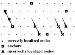
Figure 4: Experimental result

We propose some simple metrics here for performance evaluation purposes. $rate_{c}$ is the percentage of correctly localized positions, and $avg_{error}$ is the average error of the incorrectly localized positions, in terms of grid distance. In our experiment, among the 50 positions in the segment, we correctly assigned 43 nodes to their positions. Of all the other 7 positions, the errors are all just 1-hop. So in our experiment, $rate_{c}$= 86% and $avg_{error}=1$.

In [23], an algorithm is introduced to solve localization in grid wireless networks. The authors use acoustic Time Difference of Arrival (TDoA) technique for distance measurement, then use a subgraph isomorphism algorithm and topology information to calculate the result. The results they show yield a $rate_{c}$ = 88.3% and $avg_{error}=1.33$. Thus our results are comparable to the acoustic method [23], however there are advantages to using RSSI noted in the following paragraph.

Beyond the hardware expense of equipping nodes with sounder and microphone, the sounder consumes power: a buzz alone can cost energy equivalent to sending up to 50 messages, and numerous soundings are needed to overcome errors in the acoustic ranging phase. Also on the receiving end, significant signal processing is needed to process the acoustics, which can have hardware and power cost. For our table lookup algorithm, the RSSI ranging needs radio 30 messages with almost minimal signal strength. The communication energy consumption of the two methods are similar since both algorithms forward the ranging data to base station.

5 Performance Analysis

To analyze the performance, we introduce the following definitions in for 1-hop neighborhood establishment (these definitions follow the classical error terminology of hypothesis testing in statistics).

Definition 1

If two nodes $p$ and $q$ are not 1-hop neighbors, and they are considered by the algorithm to be 1-hop neighbors, then the algorithm is said to make a type A error for $(p,q)$.

Definition 2

If two nodes $p$ and $q$ are 1-hop neighbors, and they are not classified by the algorithm as 1-hop neighbors, then the algorithm is said to make a type B error for $(p,q)$.

RSSI ranging and the fuzzy membership functions effectively have thresholds between classifying a pair $(p,q)$ as 1-hop neighbors or not. Moving this threshold one way or another can change the number of type A and type B errors.

For our field experiment, among 121 1-hop pairs in the grid, we had 17 type B errors and we had 9 type A errors in 192 2-hop pairs. Among all the 50 nodes, 24 nodes have correct 1-hop neighborhoods. In other words, with the parameters we chose for the fuzzy membership functions, we recognized 86.0% of the 1-hop neighbors and took 4.7% of 2-hop neighbors for 1-hop neighbors.

Our experiment shows that we manage to reduce the number of type A and type B errors using fuzzy membership functions proposed in section 3. This result is obtained though RSSI ranging data is inaccurate. We observed that even with 30 messages in each group, the mean RSSI reading over the same distance could have a quite large variance. Distance estimation using RSSI alone can generate error as large as 60%. In our experiment, mean RSSI reading of one group of messages over distance of 10 meters can be same as the overall average reading over the distance of 16 meters. In fact, when we tried to establish the 1-hop neighborhood using RSSI distance estimation alone, and keep the type A error ratio at the similar level, we ended up having many more type B errors. The type A error ratio for 2-hop neighbors is 5.4%, and ratio of correctly recognized 1-hop neighbors is 72.2%.

Both type A and type B errors in the 1-hop neighborhood establishment can affect the tuples of the nodes. But their effects are not the same. In our topology, for most pairs of nodes, there are at least two paths of minimum length. If a type B error occurs and breaks one of the shortest paths, the distance calculation is more likely to give the same result because there are other shortest paths. In the mean time, a type A error is more likely to change the length of the shortest path. So we can see a type A error is more likely to affect the 4-tuple of a node. Thus we have the following:

Observation. The table lookup algorithm tolerates more type B errors than type A errors.

For the algorithm to achieve satisfying results, we need as few errors as possible. Unfortunately, there is a trade-off between the number of type A and type B errors. Depending on how to choose a fuzzy membership function, the score assignment and the rules to pick 1-hop number, we can reduce the number of one type of errors, but the number of the other type will increase.

We also ran simulations by injecting type A and type B errors. It turns out that to obtain good localization result, we need to reduce the number of type A errors to be fewer than 12, and number of type B errors to be fewer than 31 in the 50 node grid.

We explored the effect of segment size on the algorithm by simulations. We conducted simulations for larger segments, assuming that we could get 1-hop neighborhood information of same accuracy as in our experiment. We did simulations on segments with different sizes ranging from 50 to 200(50, 60, 70, 80, 90, 100, 150, 200). All simulations use only four anchors. For each segment size, we ran 1000 simulations. Figure 5 and 6 shows $rate_{c}$ and $avg_{error}$ for different segment sizes.

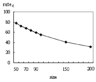
Figure 5: $rate_{c}$ for different segment sizes

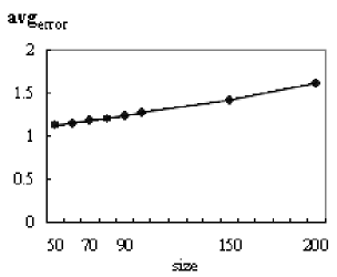
Figure 6: $avg_{error}$ for different segment sizes

With a larger segment, the accuracy of the algorithm decreases. This is because with longer paths, the errors in grid distance counting will accumulate.

6 Conclusions and Future Work

In this paper, we confirm the advantage of using a grid when an anchor-based RSSI method is used to localize a wireless sensor network. With the grid topology information, it is possible to have a simpler and better localization algorithm.

We introduced the table lookup localization algorithm and implemented it with a segment of 50 sensor nodes. The result shows that this algorithm is efficient and energy saving. Also by obtaining 1-hop neighborhood using aggregated information and fuzzy membership functions, the result is achieved with inaccurate RSSI ranging data.

There is still a lot to explore. The lower bound of 1-hop neighborhood establishment is achieved by assuming errors are mutually independent and using the current stage 3 algorithm. We can develop a more realistic model of errors to better simulate the RSSI readings, and improve the stage 3 algorithm to tolerate more errors.

References

- [1] M Anlauff and A Sunbul. Deploying localization services in wireless sensor networks. In 24th International Conference on Distributed Computing Systems Workshops, pages 782–787, March 2004.
- [2] Paramvir Bahl and Venkata N. Padmanabhan. RADAR: An in-building RF-based user location and tracking system. In INFOCOM (2), pages 775–784, 2000.
- [3] Sandip Bapat, Vinod Kulathumani, and Anish Arora. Analyzing the yield of exscal, a large-scale wireless sensor network experiment. In 13th IEEE International Conference on Network Protocols (ICNP) 2005, 2005.
- [4] P Biswas and Y Ye. Semidefinite programming for ad hoc wireless sensor network localization. In Proceedings of the third international symposium on Information processing in sensor networks (IPSN 2004), pages 46–54, 2004.
- [5] S Dolev, T Herman, and L Lahiani. Polygonal broadcast, secret maturity and the firing sensors. In Proceedings of the Third International Conference on Fun with Algorithms (FUN2004), pages 41–52, May 2004.
- [6] J Dombi. Membership function as an evaluation. Fuzzy Sets and Systems, 35:1–21, 1990.
- [7] E Elnahraway, X Li, and RP Martin. The limits of localization using rss. In Proceedings of the 2nd International Conference on Embedded Networked Sensor Systems (SENSYS 2004), pages 283–284, 2004.
- [8] A. Galstyan, B. Krishnamachari, K. Lerman1, and S. Pattem. Distributed online localization in sensor networks using a moving target. In the third international symposium on information processing in sensor networks, pages 61–70, 2004.
- [9] Tian He, Chengdu Huang Band rian M. Blum, John A. Stankovic, and Tarek Abdelzaher. Range-free localization schemes for large scale sensor networks. In MobiCom’03, pages 81–95, 2003.
- [10] Y Kwon, K Mechitov, S Sundresh, W Kim, and G Agha. Resilient localization for sensor networks in outdoor environments. In Tech. Rep. UIUCDCSR-2004-2449, 2004.
- [11] YJ Lai and CH Hwang. Fuzzy mathematical programming : methods and applications. Springer-Verlag, Berlin, 1992.
- [12] K Langendoen and N Reijers. Distributed localization in wireless sensor networks: a quantitative comparison. Computer Networks, 43:499–518, 2003.
- [13] Mario Limon Mendoza, Victor Hugo Zarate Silva, and Arturo Perez Diaz. An efficient algorithm for localization in wireless sensor networks based on internal array of nodes within cells. In ICPP Workshops, pages 405–412, 2005.
- [14] D Moore, J Leonard, D Rus, and S Teller. Robust distributed network localization with noisy range measurements. In Proceedings of the 2nd International Conference on Embedded Networked Sensor Systems (SENSYS 2004), pages 50–61, 2004.
- [15] D Niculescu and B Nath. Ad hoc positioning system. In GLOBECOM, 2001.
- [16] Dragos Niculescu and Badri Nath. Error characteristics of ad hoc positioning systems (aps). In MobiHoc 04, pages 20–30, 2004.
- [17] N Patwari and AO Hero. Using proximity and quantized rss for sensor localization in wireless networks. In WSNA ’03: Proceedings of the 2nd ACM international conference on Wireless sensor networks and applications, pages 20–29, 2003.
- [18] Rong Peng and Mihail L. Sichitiu. Robust, probabilistic, constraint-based localization for wireless sensor networks. In Second Annual IEEE Communications Society Conference on Sensor and Ad Hoc Communications and Networks (SECON 2005), 2005.
- [19] C Savarese, K Langendoen, and J Rabaey. Robust positioning algorithms for distributed ad-hoc wireless sensor network. In USENIX Technical Annual Conference, pages 317–328, 2002.
- [20] A Savvides, W Garber, S Adlakha, R Moses, and MB Srivastava. On the error characteristics of multihop node localization in ad-hoc sensor networks. In Proceedings of the second international symposium on information processing in sensor networks (IPSN 2003), pages 317–332, 2003.
- [21] A Savvides, H Park, and M Srivastava. The bits and flops of the n-hop multilateration primitive for node localization problems. In First ACM International Workshop on Wireless Sensor Networks and Application (WSNA), pages 112–121, 2002.
- [22] R. Stoleru and J. A. Stankovic. Probability grid: A location estimation scheme for wireless sensor networks. In IEEE Communications Society Conference on Sensor and Ad Hoc Communications and Networks(SECON 2004), 2004.
- [23] S Sundresh, Y Kwon, K Mechitov, W Kim, and G Agha. Localization of sparse sensor networks using layout information. In Tech. Rep. UIUCDCS-R-2005-2525, 2005.
- [24] K Whitehouse and D Culler. Calibration as parameter estimation in sensor networks. In Proceedings of the 1st ACM international workshop on Wireless sensor networks and applications, pages 59–67, 2002.
- [25] Yuecheng Zhang and Liang Cheng. Place: Protocol for location and coordinate estimation–a wireless sensor network approach. Computer Networks, 46(5):679–693, 2004.
- [26] G Zhou, T He, S Krishnamurthy, and JA Stankovic. Impact of radio irregularity on wireless sensor networks. In Proceedings of the 2nd International Conference on Mobile Systems, Applications, and Services, pages 125–138, 2004.