Geometric symmetry in the quadratic Fisher discriminant operating on image pixels

Abstract

This article examines the design of Quadratic Fisher Discriminants (QFDs) that operate directly on image pixels, when image ensembles are taken to comprise all rotated and reflected versions of distinct sample images. A procedure based on group theory is devised to identify and discard QFD coefficients made redundant by symmetry, for arbitrary sampling lattices. This procedure introduces the concept of a degeneracy matrix. Tensor representations are established for the square lattice point group (8-fold symmetry) and hexagonal lattice point group (12-fold symmetry). The analysis is largely applicable to the symmetrisation of any quadratic filter, and generalises to higher order polynomial (Volterra) filters. Experiments on square lattice sampled synthetic aperture radar (SAR) imagery verify that symmetrisation of QFDs can improve their generalisation and discrimination ability.

I Introduction

In image target detection, one often desires to detect all geometric symmetry transformed versions of targets, for two reasons. One reason is that for any given target pattern, all symmetry transformed versions also are valid target patterns, to at least a good approximation. The other reason is that so few separate target patterns are available for detector training, relative to the number of detector coefficients, that the detector has the capacity to learn the peculiarities of each individual pattern, rather than being forced to learn the universal properties of the target pattern class. Symmetry transformation of available target patterns creates additional patterns, which even if not valid target patterns, at least share many of the universal properties of genuine target patterns. Training the detector on both actual and transformed target patterns discourages overlearning of individual pattern peculiarities, and encourages learning of universal pattern properties.

There are four distinct classes of geometric point transformations: rotation; reflection; shear; and dilation. Rotation is a sense-preserving rigid-body transformation. Reflection is a sense-reversing rigid-body transformation. Shear is an angle-modifying, area-preserving transformation. Dilation is an angle-preserving, area-modifying transformation. Usually only rotation operations are considered in image target detection [1]–[4]. Reflection operations also are valid where targets have approximate mirror symmetry, or where the second reason in the previous paragraph is the motivating factor for considering symmetry. Dilation and shear have the fundamental theoretical drawback that no matter how symmetrical the detector support, there is always a flux of image content into or out of the support under these transformations, so that the detector support is not transformed onto itself. Dilations have the additional theoretical drawback for sampled (discrete) images that all strict dilations map non-lattice points onto lattice points, and all strict contractions map lattice points onto non-lattice points; once again, the discrete-space detector support is not mapped onto itself. These properties of dilation and shear preclude their inclusion in group theoretical methods of accounting for geometric symmetry in pattern recognition, as developed here and elsewhere [5]–[8]. Group theoretical considerations make rotation and reflection the only allowable geometric symmetries in this analysis. Even then, the detector support requires at least the same rotation and mirror symmetry, and orientation, as the sampling lattice, for the discrete space support to map onto itself, as it must. If one treats images as being spatially continuous and detector supports infinitely large, then dilation and shear are permissible symmetry operations [9].

This article presents the group theory based geometric symmetry analysis of the Quadratic Fisher Discriminant (QFD) operating on image pixels. Encapsulated in the analysis is a method of symmetrising any quadratic detector, not just the QFD. The mathematical formalism generalises in a straightforward manner to polynomial detectors of arbitrary degree (Volterra filters). Symmetrisation of the QFD, or indeed any polynomial filter, is a means of reducing the number of detector coefficients by identifying and discarding redundant coefficients, without introducing approximations. In contrast, most approaches to reducing polynomial filter complexity approximate the desired filter by a simpler version [10].

A synopsis of this article is as follows. Section II introduces notation and establishes the square lattice symmetry group. Section III derives the consequences for the QFD of sampling lattice symmetry. Section IV solves for the symmetrised QFD, using a procedure that is suitable for arbitrary quadratic filters, and that easily extends to higher degree polynomial filters. Section V establishes the hexagonal lattice symmetry group, and notes the detail changes in the preceding analysis if images are sampled on an hexagonal lattice instead of a square lattice. Section VI experimentally demonstrates the symmetrisation of a QFD for target detection in synthetic aperture radar (SAR) images sampled on a square lattice.

II Square lattice symmetry

As shown in Figure 1, the square lattice is generated by two equal length basis vectors subtending angle $\pi/2$. To exploit the symmetry of the sampling lattice, the detector support must be a polygon with the same symmetry as the lattice, except for translational symmetry. Conventionally, a square lattice is taken to use a square detector support of dimension $n\!\times\!n$ pixels, with total pixel count

$$N\equiv n^{2}\ ,$$ (1)

and with lattice basis vectors as perpendicular bisectors of its sides. Although not considered here, another (unusual) possibility is a square detector support centred on a lattice point and oriented so that the lattice basis vectors point at its vertices (i.e. a diamond shape).

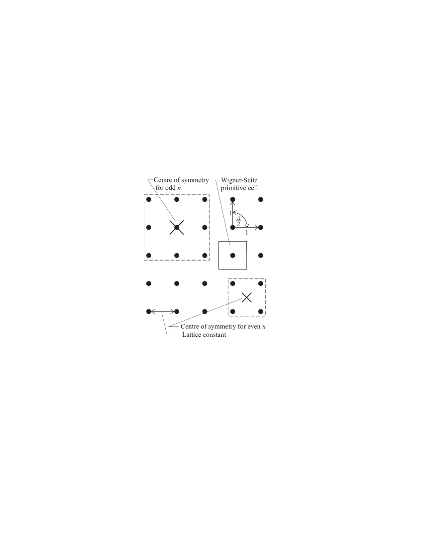
Figure 1: (Refer to Section II) A section of square lattice. Nonequivalent points marked $\times$ have identical symmetry. Detector supports of odd linear dimension centre on lattice points. Detector supports of even linear dimension centre on interstices.

The set of symmetry operations that rigidly transform a lattice onto itself while leaving one lattice point fixed, form the point group of the lattice. The fixed lattice point is the centre of symmetry. Point symmetries are restricted to rotations and reflections, since dilations and shears are prohibited for the reasons given in Section I. For a square lattice, the point group symmetry operations with centre displaced by one half lattice spacing horizontally and vertically from a lattice point, also map the square lattice onto itself, albeit without leaving any lattice point fixed (Figure 1). If the detector support has odd linear dimension (odd $n$) then it is centred on a lattice point, whereas if the detector support has even linear dimension (even $n$) then it is centred on an interstitial site. Although the two centres are not equivalent, the square lattice has identical symmetry about both centres, and that symmetry is the point symmetry.

A symmetry group $T$ having $s$ elements $T_{i}$, that is,

$$\mbox{\boldmath$T$}\equiv\{T_{1},\ldots,T_{s}\}\ ,$$ (2)

represents symmetry of order $s$ (i.e. $s$-fold symmetry). Square lattice point symmetry is of order

$$s=8\hskip 20.00003pt\mbox{(square lattice)}\ .$$ (3)

Table I lists the 8 elements of the square lattice point group—being the dihedral group $D_{4}$—in the first column. The second column of Table I describes the geometric operations corresponding to the point symmetries. Symmetries $T_{1}$ to $T_{s}$ satisfy the four mandatory group properties: closure; presence of identity element; presence of all inverse elements; and associativity. The point group is non-Abelian, because in general symmetry operations do not commute (e.g. for the square lattice point group $T_{5}\,T_{6}=T_{4}\neq\,$$T_{2}=T_{6}\,T_{5}$).

Symmetry:	Description of symmetry	Factorisation	Rank 2 tensor representation:
$T_{m}$	operation		$t^{(2)}_{m}(\{ij\};\{i^{\prime}j^{\prime}\})$
$T_{1}$	Identity or unit operation.	$T_{5}^{\,2}$	$\delta(i,i^{\prime}).$
			$\delta(j,j^{\prime})$
$T_{2}$	Anticlockwise rotation by	$T_{2}$	$\delta(i,n-j^{\prime}+1).$
	1/4 turn.		$\delta(j,i^{\prime})$
$T_{3}$	Rotation by 1/2 turn, being	$T_{2}^{\,2}$	$\delta(i,n-i^{\prime}+1).$
	inversion through centre.		$\delta(j,n-j^{\prime}+1)$
$T_{4}$	Clockwise rotation by 1/4	$T_{2}^{\,3}$	$\delta(i,j^{\prime}).$
	turn.		$\delta(j,n-i^{\prime}+1)$
$T_{5}$	Reflection in the $x$-axis.	$T_{5}$	$\delta(i,n-i^{\prime}+1).$
			$\delta(j,j^{\prime})$
$T_{6}$	Reflection in line 1/8 turn	$T_{2}\,T_{5}$	$\delta(i,n-j^{\prime}+1).$
	anticlockwise from $x$-axis.		$\delta(j,n-i^{\prime}+1)$
$T_{7}$	Reflection in the $y$-axis.	$T_{2}^{\,2}\,T_{5}$	$\delta(i,i^{\prime}).$
			$\delta(j,n-j^{\prime}+1)$
$T_{8}$	Reflection in line 1/8 turn	$T_{2}^{\,3}\,T_{5}$	$\delta(i,j^{\prime}).$
	clockwise from $x$-axis.		$\delta(j,i^{\prime})$

TABLE I: (Refer to Section II) Square lattice point group symmetry operations and their rank 2 tensor representation; the rank 4 tensor representation is derived from the rank 2 tensor representation according to (10). The detector support is square with sides of length $n$-pixels. Orientation of the lattice is such that a basis vector aligns with the $x$-axis, as in Figure 1.

Subgroups of $T$ represent image ensembles with intermediate geometric symmetry. For square lattice sampling: $\{T_{1},T_{2},T_{3},T_{4}\}$ represents a 4-fold rotation axis; $\{T_{1},T_{3},T_{5},T_{7}\}$ and $\{T_{1},T_{3},T_{6},T_{8}\}$ represent 4-fold rectangular symmetry; $\{T_{1},T_{3}\}$ represents a 2-fold rotation axis; $\{T_{1},T_{5}\}$, $\{T_{1},T_{6}\}$, $\{T_{1},T_{7}\}$ and $\{T_{1},T_{8}\}$ represent 2-fold reflection symmetry (one mirror line); and $\{T_{1}\}$ represents the complete absence of geometric symmetry. In the context of airborne surveillance, imaging in the nadir direction has the full symmetry of group $T$, but side-looking SAR only has a mirror line along the range direction ($y$-axis), corresponding to subgroup $\{T_{1},T_{7}\}$.

Introduce the 2-component index (2-index) $\{ij\}$ to convert the two indices of detector pixels (row $i$ and column $j$) into a single index,

$$\{ij\}\equiv i+(j-1)n\,:\ i,j\!\in\![1,n]\,,\ \{ij\}\!\in\![1,N]\ ,$$ (4)

thereby allowing pixels in the support to be column-ordered into the dimension $N$ column vector $x$⁽¹⁾ with components $x^{(1)}(\{ij\})$, where the (1) superscript signifies that $x$⁽¹⁾ is inherently a rank 1 tensor (i.e. vector). It is possible to construct QFD theory using 2-indices alone, at the expense of using rank 4 tensors. Alternatively, combining pairs of 2-indices ($\{ij\}$ and $\{kl\}$) into 4-component indices ($\{ij,kl\}$) according to the prescription

$$\{ij,kl\}\equiv\{ij\}+(\{kl\}-1)N\,:$$ (5)

$$\{ij\},\{kl\}\!\in\![1,N]\,,\ \{ij,kl\}\!\in\![1,N^{2}]\ ,$$

allows rank 4 tensors to be expressed as higher dimension rank 2 tensors (i.e. square matrices), as will be seen forthwith. As a reminder that 4-indices are properly a pair of 2-indices, the notation $\{ij,kl\}$ retains a comma between the first and second 2-indices. Pairwise products of pixels in the support are collected into the dimension $N^{2}$ column vector $x$⁽²⁾ with components

$$x^{(2)}(\{ij,kl\})\equiv x^{(1)}(\{ij\})\,x^{(1)}(\{kl\})\ ,$$ (6)

where the (2) superscript signifies that $x$⁽²⁾ is inherently a rank 2 tensor.

Symmetry operation $T_{m}$ linearly transforms unprimed vectors into primed vectors as follows:

$$\mbox{\boldmath$x$}^{(i)\prime}=T^{(2i)}_{m}\,\mbox{\boldmath$x$}^{(i)}\ .$$ (7)

$T^{(2)}_{m}$, with components $t^{(2)}_{m}(\{ij\};\{i^{\prime}j^{\prime}\})$, is the rank 2 tensor representation of symmetry operation $T_{m}$. $T_{m}^{(4)}$, with components $t^{(4)}_{m}(\{ij,kl\};\{i^{\prime}j^{\prime},k^{\prime}l^{\prime}\})$, is the rank 4 tensor representation of symmetry operation $T_{m}$. Use of 4-index notation allows $T_{m}^{(4)}$ to be expressed in matrix form, but this is merely a notational convenience. Lattice point symmetries rearrange image pixels without altering pixel values (i.e. they are permutation operations on the pixel values), implying invariance of the Euclidean norm

$$\mbox{\boldmath$x$}^{(i)\prime\,\mathrm{T}}\,\mbox{\boldmath$x$}^{(i)\prime}=\mbox{\boldmath$x$}^{(i)\,\mathrm{T}}\,\mbox{\boldmath$x$}^{(i)}\ ,$$ (8)

which ensures that all transformation matrices are orthogonal, that is,

$$T^{(2i)\,-1}_{m}=T^{(2i)\,\mathrm{T}}_{m}\,,\ m=1,\dots,s\ .$$ (9)

$T^{(2i)}_{m}$ have determinants 1 or $-1$. For a square lattice, $T^{(2i)}_{1}$ has eigenvalue 1, $T^{(2i)}_{3}$ and $T^{(2i)}_{5-8}$ have eigenvalues 1 and $-1$, and $T^{(2i)}_{2}$ and $T^{(2i)}_{4}$ have eigenvalues 1, $i$, $-1$ and $-i$. Expanding (7) in terms of tensor components, and substituting (6), connects components of the two representations by

$$t^{(4)}_{m}(\{ij,kl\};\{i^{\prime}j^{\prime},k^{\prime}l^{\prime}\})=t^{(2)}_{m}(\{ij\};\{i^{\prime}j^{\prime}\})\,t^{(2)}_{m}(\{kl\};\{k^{\prime}l^{\prime}\})\ .$$ (10)

Equation (10) implies that the rank 4 tensor components have permutation symmetry

$$t^{(4)}_{m}(\{ij,kl\};\{i^{\prime}j^{\prime},k^{\prime}l^{\prime}\})=t^{(4)}_{m}(\{kl,ij\};\{k^{\prime}l^{\prime},i^{\prime}j^{\prime}\})\ .$$ (11)

The rank 2 tensor representation of the square lattice point group is listed in the fourth column of Table I; the rank 4 tensor representation is computed from the rank 2 tensor representation according to (10). Each $T^{(2i)}_{m}$ matrix has a single one entry in every row and column. Computing the rank 2 tensor representation is efficiently done as follows. Derive matrices $T^{(2)}_{2}$ and $T^{(2)}_{5}$ by inspection. Elements $T_{2}$ and $T_{5}$ generate group $T$, as indicated in the third column of Table I, so the remaining elements of the rank 2 representation of $T$ are computed by repeated multiplication of matrices $T^{(2)}_{2}$ and $T^{(2)}_{5}$.

III Symmetry invariants

The underlying postulate of this analysis is that training ensemble statistics (clutter and target separately) are invariant with respect to all point symmetry transformations about the centre of detector support. Such statistical symmetry arises if every image in the actual ensemble contributes to a notional ensemble all symmetry transformations of itself (with equal weighting), and the notional ensemble is a more complete portrayal of the totality of images than the actual ensemble. There is no requirement for images in the ensembles to be individually invariant with respect to any symmetry transformations.

The quadratic detector response is given by the scalar product

$$y(\mbox{\boldmath$x$})=\mbox{\boldmath$f$}^{\mathrm{T}}\,\mbox{\boldmath$x$}\ ,$$ (12)

where detector coefficients $f$ and pixel terms $x$ partition into rank 1 and rank 2 tensors as

$$\mbox{\boldmath$f$}\equiv\left[\begin{array}[]{c}\mbox{\boldmath$f$}^{(1)}\\ \mbox{\boldmath$f$}^{(2)}\end{array}\right]\ ,\ \mbox{\boldmath$x$}\equiv\left[\begin{array}[]{c}\mbox{\boldmath$x$}^{(1)}\\ \mbox{\boldmath$x$}^{(2)}\end{array}\right]\ .$$ (13)

Pixel terms have mean

$$\begin{array}[]{l}\mbox{\boldmath$g$}=\left[\begin{array}[]{c}\mbox{\boldmath$g$}^{(1)}\\ \mbox{\boldmath$g$}^{(2)}\end{array}\right]\equiv\langle\mbox{\boldmath$x$}\rangle\;:\\[12.91663pt] \mbox{\boldmath$g$}^{(i)}\equiv\langle\mbox{\boldmath$x$}^{(i)}\rangle\ ,\end{array}$$ (14)

and covariance

$$\begin{array}[]{l}C=\left[\begin{array}[]{cc}C^{(2)}&C^{(1+2)}\\ C^{(2+1)}&C^{(4)}\end{array}\right]\equiv\left\langle(\mbox{\boldmath$x$}-\langle\mbox{\boldmath$x$}\rangle)(\mbox{\boldmath$x$}-\langle\mbox{\boldmath$x$}\rangle)^{\mathrm{T}}\right\rangle\;:\\[12.91663pt] C^{(i+j)}\equiv\left\langle(\mbox{\boldmath$x$}^{(i)}-\langle\mbox{\boldmath$x$}^{(i)}\rangle)(\mbox{\boldmath$x$}^{(j)}-\langle\mbox{\boldmath$x$}^{(j)}\rangle)^{\mathrm{T}}\right\rangle\ ,\end{array}$$ (15)

where (as usual) superscripts of the form $(i)$ indicate that the quantity is inherently a rank $i$ tensor.

					Degrees of freedom—			Degrees of freedom—
					permutation symmetry			permutation and
		Detector coefficients:			only:			geometric symmetry:
$n$	$N$	linear	quadratic	total	linear	quadratic	total	linear	quadratic	total
1	1	1	1	2	1	1	2	1	1	2
2	4	4	16	20	4	10	14	1	3	4
3	9	9	81	90	9	45	54	3	11	14
4	16	16	256	272	16	136	152	3	24	27
5	25	25	625	650	25	325	350	6	55	61
6	36	36	1296	1332	36	666	702	6	99	105
7	49	49	2401	2450	49	1225	1274	10	181	191
8	64	64	4096	4160	64	2080	2144	10	288	298
9	81	81	6561	6642	81	3321	3402	15	461	476
10	100	100	10000	10100	100	5050	5150	15	675	690
12	144	144	20736	20880	144	10440	10584	21	1368	1389
14	196	196	38416	38612	196	19306	19502	28	2499	2527
16	256	256	65536	65792	256	32896	33152	36	4224	4260
18	324	324	104976	105300	324	52650	52974	45	6723	6768
20	400	400	160000	160400	400	80200	80600	55	10200	10255
25	625	625	390625	391250	625	195625	196250	91	24805	24896

TABLE II: (Refer to Section IV) Square lattice. Reduction in degrees of freedom due to permutation symmetry and geometric symmetry. Support linear dimension is $n$, and number of pixels is $N$. The numbers of detector coefficients and degrees of freedom are resolved into linear and quadratic types.

Ensemble statistics are invariant with respect to all symmetry transformations if and only if

$$\mbox{\boldmath$g$}^{(i)}=T^{(2i)}_{m}\,\mbox{\boldmath$g$}^{(i)}\ \ \mbox{and}\ \ C^{(i+j)}=T^{(2i)}_{m}\,C^{(i+j)}\,T^{(2j)\,\mathrm{T}}_{m}\,,$$

$$m=1,\dots,s\ .$$ (16)

Using the fact that any group element multiplying separately all group elements (including itself) yields all the group elements in a different order, one may verify that

$$\begin{array}[]{l}\widetilde{\mbox{\boldmath$g$}}^{(i)}\equiv{\displaystyle\frac{1}{s}\sum_{m=1}^{s}}T^{(2i)}_{m}\,\mbox{\boldmath$g$}^{(i)}\ ,\\[17.22217pt] \widetilde{C}^{(i+j)}\equiv{\displaystyle\frac{1}{s}\sum_{m=1}^{s}}T^{(2i)}_{m}\,C^{(i+j)}\,T^{(2j)\,\mathrm{T}}_{m}\,,\end{array}$$ (17)

satisfy invariance properties (III) for arbitrary $g$⁽ⁱ⁾ and $C^{(i+j)}$. Furthermore, $\widetilde{\mbox{\boldmath$g$}}^{(i)}$ and $\widetilde{C}^{(i+j)}$ have the correct form to be ensemble statistics. Although $(\sum_{m}T^{(2i)}_{m})C^{(i+j)}(\sum_{n}T^{(2j)}_{n})$ has the correct invariance property, it is a cross-covariance between all pairs of symmetry transformed images, whereas a suitable $\widetilde{C}^{(i+j)}$ must be an autocovariance of all symmetry transformed images. The $1/s$ normalising factors in (17) ensure that if $g$⁽ⁱ⁾ and $C^{(i+j)}$ already satisfy statistics invariance conditions (III), then resymmetrisation by (17) will leave $g$⁽ⁱ⁾ and $C^{(i+j)}$ unchanged. The QFD analysis proceeds with symmetrised ensemble statistics $\widetilde{\mbox{\boldmath$g$}}^{(i)}$ and $\widetilde{C}^{(i+j)}$ in place of their unsymmetrised counterparts $g$⁽ⁱ⁾ and $C^{(i+j)}$.

The QFD is the quadratic filter whose output maximises the ratio of the squared difference of means of targets and clutter (dividend), to the sum of variances of targets and clutter (divisor). This QFD objective function is

$$\sigma(\mbox{\boldmath$f$})=\frac{\left(\mbox{\boldmath$f$}^{\mathrm{T}}\widetilde{\mbox{\boldmath$g$}}\right)^{2}}{\mbox{\boldmath$f$}^{\mathrm{T}}\widetilde{C}\mbox{\boldmath$f$}}\ ,$$ (18)

which is maximised by the solution to

$$\widetilde{C}\mbox{\boldmath$f$}=\widetilde{\mbox{\boldmath$g$}}\ .$$ (19)

In (18) and (19) $\widetilde{\mbox{\boldmath$g$}}$ is the difference of means, and $\widetilde{C}$ is the sum of covariances, for clutter and target ensembles:

$$\begin{array}[]{rcl}\widetilde{\mbox{\boldmath$g$}}&\equiv&\widetilde{\mbox{\boldmath$g$}}_{\mathrm{clutter}}-\widetilde{\mbox{\boldmath$g$}}_{\mathrm{target}}\ ,\\[8.61108pt] \widetilde{C}&\equiv&\widetilde{C}_{\mathrm{clutter}}+\widetilde{C}_{\mathrm{target}}\ .\\ \end{array}$$ (20)

Ensemble statistics invariance properties (III) applied to (19) derive detector coefficient invariance properties

$$\mbox{\boldmath$f$}^{(i)}=T^{(2i)}_{m}\,\mbox{\boldmath$f$}^{(i)}\,,\ m=1,\dots,s\ ,$$ (21)

under the assumption that $\widetilde{C}$ is nonsingular and so (19) has a unique solution. For the same reasons that apply to (17),

$$\widetilde{\mbox{\boldmath$f$}}^{(i)}=\frac{1}{s}\sum_{m=1}^{s}T^{(2i)}_{m}\,\mbox{\boldmath$f$}^{(i)}\ ,$$ (22)

satisfies invariance property (21) for arbitrary $f$⁽ⁱ⁾. Detector coefficients invariance (21) applied to (12) yields the detector response invariance property

$$y(T^{(2i)}_{m}\,\mbox{\boldmath$x$}^{(i)})=y(\mbox{\boldmath$x$}^{(i)})\,,\ m=1,\dots,s\ ,$$ (23)

which implies that the detector response is the same for all images that are point symmetry transformations of each other. Unlike this work, most approaches to filter symmetrisation [11]–[16] postulate detector response symmetry, from which detector coefficient symmetry follows.

If the argument of objective function $\sigma$ (18) is restricted to symmetrised detector coefficients $\widetilde{\mbox{\boldmath$f$}}$ (22), then explicit symmetrisation of ensemble statistics becomes redundant in the computation of $\sigma$, that is,

$$\sigma(\widetilde{\mbox{\boldmath$f$}})=\frac{\left(\widetilde{\mbox{\boldmath$f$}}^{\mathrm{T}}\widetilde{\mbox{\boldmath$g$}}\right)^{2}}{\widetilde{\mbox{\boldmath$f$}}^{\mathrm{T}}\widetilde{C}\widetilde{\mbox{\boldmath$f$}}}=\frac{\left(\widetilde{\mbox{\boldmath$f$}}^{\mathrm{T}}\mbox{\boldmath$g$}\right)^{2}}{\widetilde{\mbox{\boldmath$f$}}^{\mathrm{T}}C\widetilde{\mbox{\boldmath$f$}}}\ .$$ (24)

IV Degeneracy matrix

Solving (19) directly yields detector coefficients that are properly symmetrised to within numerical accuracy. Then if necessary, explicit symmetrisation of the detector coefficients by (22) will give perfectly symmetrised detector coefficients. However, there is a more elegant and computationally efficient method of computing perfectly symmetrised detector coefficients. This superior method introduces a degeneracy matrix to account for permutation and geometric symmetry degeneracies.

As a consequence of the group properties satisfied by matrices $T^{(2i)}_{m}$, matrix

$$D^{(2i)\prime\prime\prime}\equiv\sum_{m=1}^{s}T^{(2i)}_{m}\ ,$$ (25)

satisfies the symmetry invariance properties

$$D^{(2i)\prime\prime\prime}=T^{(2i)}_{m}\,D^{(2i)\prime\prime\prime}\,,\ m=1,\dots,s\ .$$ (26)

Matrix $D^{(2i)\prime\prime\prime}$ is symmetric,

$$D^{(2i)\prime\prime\prime\,\mathrm{T}}=D^{(2i)\prime\prime\prime}\ ,$$ (27)

due to the orthogonality property (9) of matrices $T^{(2i)}_{m}$. $D^{(2i)\prime\prime\prime}$ has nonzero entries everywhere along the main diagonal. If column $i_{1}$ has nonzero entries in rows $i_{1},i_{2},i_{3},\ldots$ (maximum of $s$ distinct rows), then columns $i_{1},i_{2},i_{3},\ldots$ are identical. The nonzero entries in a given column all have the same value and add to $s$.

Matrix $D^{(2i)\prime\prime}$ has a one entry wherever $D^{(2i)\prime\prime\prime}$ has any nonzero entry:

$$d^{(2i)\prime\prime}(k^{(i)};l^{(i)})\equiv\left\{\begin{array}[]{l}1\ \mbox{if}\ d^{(2i)\prime\prime\prime}(k^{(i)};l^{(i)})\neq 0\\ 0\ \mbox{otherwise}\end{array}\right.\ ,$$ (28)

where the notation $k^{(i)}$ is an abbreviation for a $2i$-component index. Matrix $D^{(2i)\prime\prime}$ is symmetric. Because each matrix $T^{(2i)}_{m}$ contains only a single one entry per row or column, and zeros elsewhere, $D^{(2i)\prime\prime}$ satisfies the symmetry invariance properties

$$D^{(2i)\prime\prime}=T^{(2i)}_{m}\,D^{(2i)\prime\prime}\,,\ m=1,\dots,s\ .$$ (29)

Additional to the geometric symmetry being postulated in this analysis, it is convenient to impose the permutation symmetry

$$f^{(2)}(\{ij,kl\})=f^{(2)}(\{kl,ij\})$$ (30)

on the rank 2 tensor detector coefficients. Permutation symmetry (30) of $f$⁽²⁾ is chosen to correspond to the permutation symmetry of $x$⁽²⁾ (6). Matrix $D^{(4)\prime}$ has a one entry if $D^{(4)\prime\prime}$ has a one entry at the same row and column, or the same row but permuted column 4-index:

$$d^{(4)\prime}(\{ij,kl\};\{i^{\prime}j^{\prime},k^{\prime}l^{\prime}\})\equiv$$ (34)

$$\left\{\begin{array}[]{l}1\ \mbox{if}\ d^{(4)\prime\prime}(\{ij,kl\};\{i^{\prime}j^{\prime},k^{\prime}l^{\prime}\})=1\ \mbox{or}\\ \phantom{1\ \mbox{if}\ }d^{(4)\prime\prime}(\{ij,kl\};\{k^{\prime}l^{\prime},i^{\prime}j^{\prime}\})=1\\[4.30554pt] 0\ \mbox{otherwise}\end{array}\right.\ .$$

$D^{(4)\prime}$ satisfies the geometric symmetry invariance properties

$$D^{(4)\prime}=T^{(4)}_{m}\,D^{(4)\prime}\,,\ m=1,\dots,s\ ,$$ (35)

and the permutation symmetry invariance properties

$$\begin{array}[]{l}d^{(4)\prime}(\{ij,kl\};\{i^{\prime}j^{\prime},k^{\prime}l^{\prime}\})=d^{(4)\prime}(\{ij,kl\};\{k^{\prime}l^{\prime},i^{\prime}j^{\prime}\})=\\[4.30554pt] d^{(4)\prime}(\{kl,ij\};\{i^{\prime}j^{\prime},k^{\prime}l^{\prime}\})=d^{(4)\prime}(\{kl,ij\};\{k^{\prime}l^{\prime},i^{\prime}j^{\prime}\})\ .\end{array}$$ (36)

Additional to (36) is the property that $D^{(4)\prime}$ is a symmetric matrix, which may be regarded as another, unavoidable permutation symmetry. The redefinition

$$D^{(2)\prime}\equiv D^{(2)\prime\prime}\ ,$$ (37)

is adopted for notational consistency. Covariance matrix $C$ and its derivatives have multiple essential singularities if permutation symmetry is not explicitly taken into account, as is done here by replacing $D^{(2i)\prime\prime}$ by $D^{(2i)\prime}$.

Figure 2: (Refer to Section V) A section of hexagonal lattice. Nonequivalent points marked $\times$ correspond to different symmetries—lattice points have hexagonal symmetry, and interstitial sites have triangular symmetry. Shown is a detector support of linear dimension $n$, and the pixel indexing scheme.

Define the reduced width matrix $D^{(2i)}$ as having columns that are all of the distinct columns of matrix $D^{(2i)\prime}$, without repetition. Repeated columns in $D^{(2i)\prime}$ are identified by the property that if column $i_{1}$ has one entries in rows $i_{1},i_{2},i_{3},\ldots$, then columns $i_{1},i_{2},i_{3},\ldots$ are identical, and there are no other columns that are identical to column $i_{1}$. This property derives from the analogous property of $D^{(2i)\prime\prime\prime}$ that was noted earlier in this section. Matrices $D^{(2)}$ and $D^{(4)}$ respectively are the rank 2 and rank 4 tensor parts of degeneracy matrix $D$:

$$D\equiv\left[\begin{array}[]{cc}D^{(2)}&0\\ 0&D^{(4)}\end{array}\right]\ .$$ (38)

$D^{(2i)}$ satisfies the geometric symmetry invariance properties

$$D^{(2i)}=T^{(2i)}_{m}\,D^{(2i)}\,,\ m=1,\dots,s\ ,$$ (39)

and the permutation symmetry invariance properties

$$d^{(4)}(\{ij,kl\};m)=d^{(4)}(\{kl,ij\};m)\ .$$ (40)

Symmetry:	Description of symmetry	Factorisation	Rank 2 tensor representation:
$T_{m}$	operation		$t^{(2)}_{m}(\{ij\};\{i^{\prime}j^{\prime}\})$
$T_{1}$	Identity or unit operation.	$T_{7}^{\,2}$	$\delta(i,i^{\prime}).$
			$\delta(j,j^{\prime})$
$T_{2}$	Anticlockwise rotation by	$T_{2}$	$\delta(i,(i^{\prime}+j^{\prime}-2)\bmod 6(j^{\prime}-1)+1).$
	1/6 turn.		$\delta(j,j^{\prime})$
$T_{3}$	Anticlockwise rotation by	$T_{2}^{\,2}$	$\delta(i,(i^{\prime}+2j^{\prime}-3)\bmod 6(j^{\prime}-1)+1).$
	1/3 turn.		$\delta(j,j^{\prime})$
$T_{4}$	Rotation by 1/2 turn, being	$T_{2}^{\,3}$	$\delta(i,(i^{\prime}+3j^{\prime}-4)\bmod 6(j^{\prime}-1)+1).$
	inversion through centre.		$\delta(j,j^{\prime})$
$T_{5}$	Clockwise rotation by 1/3	$T_{2}^{\,4}$	$\delta(i,(i^{\prime}+4j^{\prime}-5)\bmod 6(j^{\prime}-1)+1).$
	turn.		$\delta(j,j^{\prime})$
$T_{6}$	Clockwise rotation by 1/6	$T_{2}^{\,5}$	$\delta(i,(i^{\prime}+5j^{\prime}-6)\bmod 6(j^{\prime}-1)+1).$
	turn.		$\delta(j,j^{\prime})$
$T_{7}$	Reflection in the $x$-axis.	$T_{7}$	$\delta(i,(6j^{\prime}-i^{\prime}-5)\bmod 6(j^{\prime}-1)+1).$
			$\delta(j,j^{\prime})$
$T_{8}$	Reflection in line 1/12 turn	$T_{2}\,T_{7}$	$\delta(i,(7j^{\prime}-i^{\prime}-6)\bmod 6(j^{\prime}-1)+1).$
	anticlockwise from $x$-axis.		$\delta(j,j^{\prime})$
$T_{9}$	Reflection in line 1/6 turn	$T_{2}^{\,2}\,T_{7}$	$\delta(i,(8j^{\prime}-i^{\prime}-7)\bmod 6(j^{\prime}-1)+1).$
	anticlockwise from $x$-axis.		$\delta(j,j^{\prime})$
$T_{10}$	Reflection in the $y$-axis.	$T_{2}^{\,3}\,T_{7}$	$\delta(i,(9j^{\prime}-i^{\prime}-8)\bmod 6(j^{\prime}-1)+1).$
			$\delta(j,j^{\prime})$
$T_{11}$	Reflection in line 1/6 turn	$T_{2}^{\,4}\,T_{7}$	$\delta(i,(10j^{\prime}-i^{\prime}-9)\bmod 6(j^{\prime}-1)+1).$
	clockwise from $x$-axis.		$\delta(j,j^{\prime})$
$T_{12}$	Reflection in line 1/12 turn	$T_{2}^{\,5}\,T_{7}$	$\delta(i,(11j^{\prime}-i^{\prime}-10)\bmod 6(j^{\prime}-1)+1).$
	clockwise from $x$-axis.		$\delta(j,j^{\prime})$

TABLE III: (Refer to Section V) Hexagonal lattice point group symmetry operations and their rank 2 tensor representation; the rank 4 tensor representation is derived from the rank 2 tensor representation according to (10). Orientation of the lattice is such that a basis vector aligns with the $x$ axis, as in Figure 2. Note that the modulo operation is always with respect to $6(j^{\prime}-1)$.

Let $\widehat{\mbox{\boldmath$f$}}$ be an unconstrained nondegenerate detector coefficient vector. Then

$$\widetilde{\mbox{\boldmath$f$}}=D\widehat{\mbox{\boldmath$f$}}$$ (41)

is a degenerate coefficient vector that has both the required geometric symmetry (21) and permutation symmetry (30). Each row of matrix $D$ has a single one entry and zeros elsewhere. Multiple one entries in a column of $D$ associate degenerate coefficients in the symmetrised detector $\widetilde{\mbox{\boldmath$f$}}$. The number of columns in $D$, and the number of components in $\widehat{\mbox{\boldmath$f$}}$, is the number of degrees of freedom of the detector. Substituting (41) into (24) re-expresses the objective function as

$$\sigma(\widehat{\mbox{\boldmath$f$}})=\frac{\left(\widehat{\mbox{\boldmath$f$}}^{\mathrm{T}}\widehat{\mbox{\boldmath$g$}}\right)^{2}}{\widehat{\mbox{\boldmath$f$}}^{\mathrm{T}}\widehat{C}\widehat{\mbox{\boldmath$f$}}}\ ,$$ (42)

where the nondegenerate mean vector $\widehat{\mbox{\boldmath$g$}}$ is

$$\widehat{\mbox{\boldmath$g$}}\equiv D^{\mathrm{T}}\widetilde{\mbox{\boldmath$g$}}=D^{\mathrm{T}}\mbox{\boldmath$g$}\ ,$$ (43)

and the nondegenerate covariance matrix $\widehat{C}$ is

$$\widehat{C}\equiv D^{\mathrm{T}}\widetilde{C}D=D^{\mathrm{T}}CD\ .$$ (44)

The second equalities in (43) and (44), which also may be derived from (17) and (39), affirm the redundancy of statistics symmetrisation already noted in association with (24). Equation (44) shows that the degeneracy matrix formalism maximally compresses the covariance matrix without loss of information; an alternative approach due to Lenz [17, 18] partially compresses the covariance matrix into an equal size block diagonal matrix, whose top-left block has precisely the same size as $\widehat{C}$ of (44).

Maximisation of objective function (42) is equivalent to solving (cf. (19))

$$\widehat{C}\widehat{\mbox{\boldmath$f$}}=\widehat{\mbox{\boldmath$g$}}\ ,$$ (45)

whose solution is

$$\widehat{\mbox{\boldmath$f$}}=\widehat{C}^{{\dagger}}\widehat{\mbox{\boldmath$g$}}\ ,$$ (46)

where $\widehat{C}^{{\dagger}}$ is the Moore-Penrose generalised inverse (or pseudoinverse) [19] of $\widehat{\mbox{$C$}}$. A property of solutions of the form (46) obtained by generalised inversion is that they are the minimum norm vector that minimises the Euclidean norm of the residual $(\widehat{C}\widehat{\mbox{\boldmath$f$}}-\widehat{\mbox{\boldmath$g$}})$ [20]. The residual vanishes if $\widehat{\mbox{$C$}}$ is nonsingular, in which case the generalised inverse is equivalent to the conventional inverse. QFD generalisation may be improved by regularising $\widehat{\mbox{$C$}}$ [21, 22] before solving (45).

A necessary and sufficient condition for $\widehat{C}$ to be nonsingular is that the clutter and target training ensembles between them must contain no fewer linearly independent images than the number of symmetrised detector degrees of freedom. In contrast, symmetrised covariance matrix $\widetilde{C}$ (and unsymmetrised covariance matrix $C$) contains many essential singularities, no matter how large the training ensembles. Zero eigenvalues of $\widetilde{C}$ are at least equal in number to the number of permutation symmetry degeneracies in the detector coefficients; beyond that there may be extra zero eigenvalues due to small training ensemble sizes. The present degeneracy matrix removes the essential singularities in $\widetilde{C}$ or $C$ by operation (44).

Table II shows the reduction in degrees of freedom afforded by permutation and geometric symmetries. Permutation symmetry among the $N\!+\!N^{2}$ coefficients leaves $N\!+\!N(N\!+\!1)/2$ degrees of freedom. This is a reduction in degrees of freedom by a factor of up to 2. Maximum reduction is achieved for large detector supports, where the proportion of quadratic terms that are pixel self-products becomes small. Geometric symmetry further reduces the degrees of freedom by a factor of up to $s$ ($s\!=\!8$ for a square lattice, to which Table II applies). Maximum reduction occurs for large detector supports, where proportionately few pixels and pixel pairs map onto either themselves under symmetry transformations, or common pixels or pixel pairs under different symmetry transformations. The reduction in degrees of freedom attributable to geometric symmetry should constitute a significant improvement in detector generalisation, when the unsymmetrised detector generalises poorly.

V Hexagonal lattice symmetry

					Degrees of freedom—			Degrees of freedom—
					permutation symmetry			permutation and
		Detector coefficients:			only:			geometric symmetry:
$n$	$N$	linear	quadratic	total	linear	quadratic	total	linear	quadratic	total
1	1	1	1	2	1	1	2	1	1	2
2	7	7	49	56	7	28	35	2	6	8
3	19	19	361	380	19	190	209	4	26	30
4	37	37	1369	1406	37	703	740	6	77	83
5	61	61	3721	3782	61	1891	1952	9	189	198
6	91	91	8281	8372	91	4186	4277	12	394	406
7	127	127	16129	16256	127	8128	8255	16	742	758
8	169	169	28561	28730	169	14365	14534	20	1281	1301
9	217	217	47089	47306	217	23653	23870	25	2081	2106
10	271	271	73441	73712	271	36856	37127	30	3206	3236
11	331	331	109561	109892	331	54946	55277	36	4746	4782
12	397	397	157609	158006	397	79003	79400	42	6781	6823
13	469	469	219961	220430	469	110215	110684	49	9421	9470
14	547	547	299209	299756	547	149878	150425	56	12762	12818
15	631	631	398161	398792	631	199396	200027	64	16934	16998

TABLE IV: (Refer to Section V) Hexagonal lattice. Reduction in degrees of freedom due to permutation symmetry and geometric symmetry. Support linear dimension is $n$, and number of pixels is $N$. The numbers of detector coefficients and degrees of freedom are resolved into linear and quadratic types.

The most symmetric possible plane lattice has a 6-fold rotation axis through a lattice point, around which are 6 mirror lines in the lattice plane uniformly spaced by angle $\pi/6$; this lattice is the hexagonal lattice. As shown in Figure 2, the hexagonal lattice is generated by two equal length basis vectors subtending angle $\pi/3$. With centre of symmetry at a lattice point, hexagonal lattice point symmetry is of order

$$s=12\hskip 20.00003pt\mbox{(hexagonal lattice)}\ .$$ (47)

Unlike the square lattice, interstitual sites in the hexagonal lattice have reduced symmetry compared with lattice point centres. The 6-fold point symmetry of hexagonal lattice interstices is even lower than the 8-fold point symmetry of square lattices. Clearly, one would not sample on an hexagonal lattice, only to use detector supports centred on interstices. Having established that the detector support will be centred only on lattice points, Figure 2 shows a regular hexagonal support of linear dimension $n$, and a suitable pixel indexing scheme. The support linear dimension $n$ is the number of concentric hexagons that account for all pixels, where the central lattice point counts as a hexagon of vanishing size; equivalently, the linear dimension is the number of lattice points between adjacent vertices of the support perimeter. A spiral indexing scheme is adopted for the hexagonal lattice, where $(i,j)$ represents the $i$th lattice point in the $j$th concentric hexagon. An analogous spiral indexing scheme could have been used for the square lattice, the result being a closer correspondence between the point symmetry tensor representations for square and hexagonal lattices than is evident in comparing Tables I and III. The row-column indexing scheme actually used for the square lattice in Table I is conventional, and allows simpler expression of tensor representations, as is evident in comparing Tables I and III.

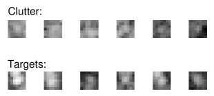
Figure 3: (Refer to Section VI) Sample clutter and target $9\!\times\!9$ image chips as used in the experiment.

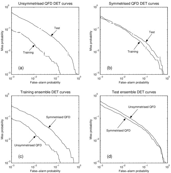
Figure 4: (Refer to Section VI) Training and test ensemble DET curves of the unsymmetrised and symmetrised QFDs, plotted in various combinations to aid comparison. Dual axis error bars are shown in graphs (a) and (b).

The square lattice analysis of Section II also holds for the hexagonal lattice, with the following detail amendments. The total number of pixels in the hexagonal support is (c.f. (1))

$$N\equiv 1+3n(n-1)\ .$$ (48)

Radial index $j$ and circumferential index $i$ transform to 2-component index $\{ij\}$ according to (c.f. 4)

$$\begin{array}[]{c}\{ij\}\equiv i+\min(1,j-1)+3(j-2)(j-1)\ :\\ j\in[1,n]\ ,\ i\in[1,\max(6(j-1),1)]\ ,\ \{ij\}\in[1,N]\ .\end{array}$$ (49)

Details of the hexagonal lattice point group—being the dihedral group $D_{6}$—are presented in Table III (c.f. Table I). Point subgroups of the hexagonal lattice are: $\{T_{1},T_{2},T_{3},T_{4},T_{5},T_{6}\}$ representing a 6-fold rotation axis; $\{T_{1},T_{3},T_{5},T_{7},T_{9},T_{11}\}$ and $\{T_{1},T_{3},T_{5},T_{8},T_{10},T_{12}\}$ representing 6-fold triangular symmetry; $\{T_{1},T_{3},T_{5}\}$ representing a 3-fold rotation axis; $\{T_{1},T_{7}\}$, $\{T_{1},T_{8}\}$, $\{T_{1},T_{9}\}$, $\{T_{1},T_{10}\}$, $\{T_{1},T_{11}\}$ and $\{T_{1},T_{12}\}$ representing 2-fold reflection symmetry (one mirror line); and $\{T_{1}\}$ representing complete absence of geometric symmetry. Depending on the degree of symmetry of the continuous image ensembles, it may or may not be beneficial to use hexagonal sampling instead of square sampling. For an hexagonal lattice, $T^{(2i)}_{1}$ has eigenvalue 1, $T^{(2i)}_{4}$ and $T^{(2i)}_{7-12}$ have eigenvalues 1 and $-1$, $T^{(2i)}_{3}$ and $T^{(2i)}_{5}$ have eigenvalues 1 and $-1/2\pm\sqrt{3}/2i$, and $T^{(2i)}_{2}$ and $T^{(2i)}_{6}$ have eigenvalues $\pm 1$, $1/2\pm\sqrt{3}/2i$, and $-1/2\pm\sqrt{3}/2i$. The only amendment to the degeneracy matrix analysis of Section IV is that for the hexagonal lattice columns of $D^{(2)\prime\prime\prime}$ have either 12 1s, or 6 2s, or 1 12 entry; likewise for $D^{(4)\prime\prime\prime}$ with the inclusion of columns with 3 4 entries. Columns with 4 3s or 2 6s, although plausible on number theoretical grounds, never occur in $D^{(2i)\prime\prime\prime}$ (c.f. Footnote 14).

Reduction in detector degrees of freedom consequent on hexagonal lattice permutation and geometric symmetries is quantified in Table IV (c.f. Table II). Support linear dimensions are quantified by $n$ for both square and hexagonal lattices, but $n$ is akin to the support diameter for the square lattice and radius for the hexagonal lattice. Accordingly, square and hexagonal supports with the same $n$ contain very different numbers of pixels—almost 3 times more in the hexagonal support for large $n$. A hexagonal support of linear dimension $n$ is closer in pixel population to a square support of linear dimension $2n$—just over 1/3 more in the square support for large $n$. Permutation symmetry reduces degrees of freedom by a factor of almost 2 for larger supports, for both square and hexagonal lattices. Geometric symmetry reduces degrees of freedom by a factor of almost $s$ for large supports, for both square and hexagonal lattices. The hexagonal lattice, with $s\!=\!12$, achieves greater reduction in degrees of freedom than the square lattice, with $s\!=\!8$.

VI Experimental results

The effect of QFD symmetrisation on target detection in real imagery is investigated. Discrimination is between SAR images of bushland and SAR images of a variety of vehicles immersed in the same bushland, samples of which are shown in Figure 3. Images are sampled on a square lattice. Image ensembles are a mixture of different flights of a spotlight SAR illuminating the ground at different angles of incidence. Clutter images are not just random samples of the background, but are background regions that ‘tricked’ a simple prescreener into declaring a target; hence the difficulty of distinguishing between clutter and targets in Figure 3. In these experiments ensemble sizes are: clutter training—17197 ; clutter test—37909 ; target training—3425 ; target test—3579. Detector support is $9\!\times\!9$ pixels, so $n\!=\!9$. Unsymmetrised and symmetrised QFDs are computed by the same procedure, but using different degeneracy matrices $D$. The unsymmetrised detector degeneracy matrix accounts for only permutation symmetry, while the symmetrised detector degeneracy matrix accounts for the full 8-fold square lattice point symmetry as well as permutation symmetry. It has been noted in Section II that square lattice sampled SAR image ensembles strictly have only 2-fold symmetry, so in principle the detector is being excessively symmetrised here. Justification for maximally symmetrising the detector is that SAR image ensembles have approximately 8-fold symmetry, and that imposing the full 8-fold symmetrisation on the detector allows verification of the full square lattice point group representation tabulated in Table I. However, there is a risk that the excessive symmetrisation will reduce the detector effectiveness compared with its unsymmetrised counterpart.

Experimental ‘detection error trade-off’ (DET) curves are plotted in Figure 4 in various combinations to assist comparison. Error bars ($\pm 1$ standard deviation) are plotted in graphs that compare training and test ensemble DET curves (i.e. graphs (a) and (b)). Graph (a) demonstrates that the unsymmetrised QFD generalises poorly, while graph (b) demonstrates that the symmetrised QFD generalises well. The reason for this behaviour is revealed in Table II, which states that the unsymmetrised QFD has 3402 degrees of freedom compared with the 476 of the symmetrised QFD. There is more scope for the unsymmetrised QFD to overtrain on the training ensemble than there is for the symmetrised QFD, as is apparent in graph (c). That the unsymmetrised QFD is going to generalise poorly in this example, is predictable beforehand on the basis of the number of detector degrees of freedom (3402) not being much less than the size of the smaller of the target and clutter training ensembles (3425). Both unsymmetrised and symmetrised detectors should have their generalisation improved by regularisation procedures [21, 22]. Graph (d) demonstrates that—despite the caution expressed at the end of the previous paragraph—the symmetrised QFD is more effective than the unsymmetrised QFD when tested on the test ensembles, and the advantage is most pronounced at the important low false-alarm probabilty extreme of the DET. The correctness of the square lattice point group representation tabulated in Table I has been verified, and the practical value of QFD symmetrisation—even theoretically excessive symmetrisation—has been established.

Robert Caprari was awarded a Bachelor of Engineering (Honours) degree in electrical and electronic engineering, and a Bachelor of Science degree, from Adelaide University. He was awarded a Doctor of Philosophy degree in physics from Flinders University, where his doctoral research was in electron scattering and condensed matter physics. All of his professional career has been spent as a research scientist with the Defence Science and Technology Organisation (DSTO) in Australia. Within DSTO, his research has broadly been in the fields of signal theory, image processing, pattern recognition and statistical learning.

References

- [1] Y.-N. Hsu, H. Arsenault and G. April, “Rotation-invariant digital pattern recognition using circular harmonic expansion”, Appl. Opt. 21, 4012–4015 (1982).
- [2] R. Wu and H. Stark, “Rotation-invariant pattern recognition using optimum feature extraction”, Appl. Opt. 24, 179–184 (1985).
- [3] C.-F. Chiu and C.-Y. Wu, “The design of rotation-invariant pattern recognition using the silicon retina”, IEEE J. Sol.-State Circ. 32, 526–534 (1997).
- [4] M. Fukumi, S. Omatu and Y. Nishikawa, “Rotation-invariant neural pattern recognition system estimating a rotation angle”, IEEE Trans. Neur. Net. 8, 568–581 (1997).
- [5] R. Lenz, “Group-theoretical model of feature extraction”, J. Opt. Soc. Am. A 6, 827–834 (1989).
- [6] R. Lenz, “Group invariant pattern recognition”, Patt. Recog. 23, 199–217 (1990).
- [7] R. Lenz, Group Theoretical Methods in Image Processing, Springer-Verlag, Berlin (1990).
- [8] Y. Liu, R. Collins and Y. Tsin, “A computational model for periodic pattern perception based on frieze and wallpaper groups”, IEEE Trans. Pattern Anal. Mach. Intell. 26, 354–371 (2004).
- [9] T. Leen, “From data distributions to regularization in invariant learning”, Neural Comp. 7, 974–981 (1995).
- [10] R. Nowak and B. Van Veen, “Tensor product basis approximations for Volterra filters”, IEEE Trans. Signal Process. 44, 36–50 (1996).
- [11] C. Giles and T. Maxwell, “Learning, invariance, and generalization in high-order neural networks”, Appl. Opt. 26, 4972–4978 (1987).
- [12] G. Ramponi and G. Sicuranza, “Quadratic digital filters for image processing”, IEEE Trans. Acoust., Speech, Signal Process. 36, 937–939 (1988).
- [13] M. Reid, L. Spirkovska and E. Ochoa, “Simultaneous position, scale, and rotation invariant pattern classification using third-order neural networks”, Neural Net. 1, 154–158 (1989).
- [14] G. Ramponi, “Bi-impulse response design of isotropic quadratic filters”, Proc. IEEE 78, 665–677 (1990).
- [15] G. Gheen, “Distortion invariant Volterra filters”, Pattern Recog. 27, 569–576 (1994).
- [16] T. Sams and J. Hansen, “Implications of physical symmetries in adaptive image classifiers”, Neural Net. 13, 565–570 (2000).
- [17] R. Lenz, “Using representations of the dihedral groups in the design of early vision filters”, ICASSP-93, V165–V167 (1993).
- [18] R. Lenz, “Investigation of receptive fields using represenations of the dihedral groups”, J. Vis. Commun. Image Rep. 6, 209–227 (1995).
- [19] R. Penrose, “A generalized inverse for matrices”, Proc. Camb. Phil. Soc. 51, 406–413 (1955).
- [20] R. Penrose, “On best approximate solutions of linear matrix equations”, Proc. Camb. Phil. Soc. 52, 17–19 (1956).
- [21] J. Friedman, “Regularized discriminant analysis”, J. Am. Statist. Assoc. 84, 165–175 (1989).
- [22] T. Hastie, A. Buja and R. Tibshirani, “Penalized discriminant analysis”, Ann. Stat. 23, 73–102 (1995).