Abstract

A simple scheme for communication over MIMO broadcast channels is introduced which adopts the lattice reduction technique to improve the naive channel inversion method. Lattice basis reduction helps us to reduce the average transmitted energy by modifying the region which includes the constellation points. Simulation results show that the proposed scheme performs well, and as compared to the more complex methods (such as the perturbation method [1]) has a negligible loss. Moreover, the proposed method is extended to the case of different rates for different users. The asymptotic behavior (SNR$\longrightarrow\infty$) of the symbol error rate of the proposed method and the perturbation technique, and also the outage probability for the case of fixed-rate users is analyzed. It is shown that the proposed method, based on LLL lattice reduction, achieves the optimum asymptotic slope of symbol-error-rate (called the precoding diversity). Also, the outage probability for the case of fixed sum-rate is analyzed.

I Introduction

In the recent years, communications over multiple-antenna fading channels has attracted the attention of many researchers. Initially, the main interest has been on the point-to-point Multiple-Input Multiple-Output (MIMO) communications [2, 3, 4, 5, 6]. In [2] and [3], the authors have shown that the capacity of a MIMO point-to-point channel increases linearly with the minimum number of the transmit and the receive antennas.

More recently, new information theoretic results [7], [8], [9], [10] have shown that in multiuser MIMO systems, one can exploit most of the advantages of multiple-antenna systems. It has been shown that in a MIMO broadcast system, the sum-capacity grows linearly with the minimum number of the transmit and receive antennas [8], [9], [10]. To achieve the sum capacity, some information theoretic schemes, based on dirty-paper coding, are introduced. Dirty-paper coding was originally proposed for the Gaussian interference channel when the interfering signal is known at the transmitter [11]. Some methods, such as using nested lattices, are introduced as practical techniques to achieve the sum-capacity promised by the dirty-paper coding [12]. However, these methods are not easy to implement.

As a simple precoding scheme for MIMO broadcast systems, the channel inversion technique (or zero-forcing beamforming [7]) can be used at the transmitter to separate the data for different users. To improve the performance of the channel inversion technique, a zero-forcing approximation of the dirty paper coding (based on QR decomposition) is introduced in [7] (which can be seen as a scalar approximation of [12]). However, both of these methods are vulnerable to the poor channel conditions, due to the occasional near-singularity of the channel matrix (when the channel matrix has at least one small eigenvalue). This drawback results in a poor performance in terms of the symbol-error-rate for the mentioned methods [1].

In [1], the authors have introduced a vector perturbation technique which has a good performance in terms of symbol error rate. Nonetheless, this technique requires a lattice decoder which is an NP-hard problem. To reduce the complexity of the lattice decoder, in [13, 14, 15, 16], the authors have used lattice-basis reduction to approximate the closest lattice point (using Babai approximation).

In this paper, we present a transmission technique for the MIMO broadcast channel based on the lattice-basis reduction. Instead of approximating the closest lattice point in the perturbation problem, we use the lattice-basis reduction to reduce the average transmitted energy by reducing the second moment of the fundamental region generated by the lattice basis. This viewpoint helps us to: (i) achieve a better performance as compared to [14], (ii) expand the idea for the case of unequal-rate transmission, and (iii) obtain some analytic results for the asymptotic behavior (SNR$\longrightarrow\infty$) of the symbol-error-rate for both the proposed technique and the perturbation technique of [1].

The rest of the paper is organized as the following: Sections II and III briefly describe the system model and introduce the concept of lattice basis reduction. In section IV, the proposed method is described and in section V, the proposed approach is extended for the case of unequal-rate transmission. In section VI, we consider the asymptotic performance of the proposed method for high SNR values, in terms of the probability of error. We define the precoding diversity and the outage probability for the case of fixed-rate users. It is shown that by using lattice basis reduction, we can achieve the maximum precoding diversity. For the proof, we use a bound on the orthogonal deficiency of an LLL-reduced basis. Also, an upper bound is given for the probability that the length of the shortest vector of a lattice (generated by complex Gaussian vectors) is smaller than a given value. Using this result, we also show that the perturbation technique achieves the maximum precoding diversity. In section VII, some simulation results are presented. These results show that the proposed method offers almost the same performance as [1] with a much smaller complexity. As compared to [14], the proposed method offers almost the same performance. However, by sending a very small amount of side information (a few bits for one fading block), the modified proposed method offers a better performance with a similar complexity. Finally, in section VIII, some concluding remarks are presented.

II System Model and Problem Formulation

We consider a multiple-antenna broadcast system with $N_{t}$ transmit antennas and $N_{r}$ single-antenna users ($N_{t}\geq N_{r}$). Consider $\mathbf{y}=[y_{1},...,y_{N_{r}}]^{T}$, $\mathbf{x}=[x_{1},...,x_{N_{t}}]^{T}$, $\mathbf{w}=[w_{1},...,w_{N_{r}}]^{T}$, and the $N_{r}\times N_{t}$ matrix $\mathbf{H}$, respectively, as the received signal, the transmitted signal, the noise vector, and the channel matrix. The transmission over the channel can be formulated as,

$$\mathbf{y}=\mathbf{H}\mathbf{x}+\mathbf{w}.$$ (1)

The channel is assumed to be Raleigh, i.e. the elements of $\mathbf{H}$ are i.i.d. with the zero-mean unit-variance complex Gaussian distribution and the noise is i.i.d. additive Gaussian. Moreover, we have the energy constraint on the transmitted signal, $\textmd{E}(\|\mathbf{x}\|^{2})=1$. The energy of the additive noise is $\sigma^{2}$ per antenna, i.e. $\textmd{E}(\|\mathbf{w}\|^{2})=N_{r}\sigma^{2}$. The Signal-to-Noise Ratio (SNR) is defined as $\rho=\frac{1}{\sigma^{2}}$.

In a broadcast system, the receivers do not cooperate with each other (they should decode their respective data, independently). The main strategy in dealing with this restriction is to apply an appropriate precoding scheme at the transmitter. The simplest method in this category is using the channel inversion technique at the transmitter to separate the data for different users:

$$\mathbf{s}=\mathbf{H}^{+}\mathbf{u},$$ (2)

where $\mathbf{H}^{+}=\mathbf{H}^{\mathtt{H}}(\mathbf{H}\mathbf{H}^{\mathtt{H}})^{-1}$, and $\mathbf{H}^{\mathtt{H}}$ is the Hermitian of $\mathbf{H}$. Moreover, $\mathbf{s}$ is the transmitted signal before the normalization ($\mathbf{x}=\dfrac{\mathbf{s}}{\sqrt{\textmd{E}(\|\mathbf{s}\|^{2})}}$ is the normalized transmitted signal), and $\mathbf{u}$ is the data vector, i.e. $u_{i}$ is the data for the i’th user. For $N_{t}=N_{r}$ (the number of transmit antennas and the number of users are equal), the transmitted signal is

$$\mathbf{s}=\mathbf{H}^{-1}\mathbf{u}.$$ (3)

The problem arises when $\mathbf{H}$ is poorly conditioned and $\|\mathbf{s}\|$ becomes very large, resulting in a high power consumption. This situation occurs when at least one of the singular values of $\mathbf{H}$ is very small which results in vectors with large norms as the columns of $\mathbf{H}^{+}$. Fortunately, most of the time (especially for high SNRs), we can combat the effect of a small singular value by changing the supporting region of the constellation which is the main motivation behind the current article.

When the data of different users are selected from $\mathbb{Z}[i]$, the overall constellation can be seen as a set of lattice points. In this case, lattice algorithms can be used to modify the constellation. Especially, lattice-basis reduction is a natural solution for modifying the supporting region of the constellation.

III Lattice-Basis Reduction

Lattice structures have been frequently used in different communication applications such as quantization or decoding of MIMO systems. A real (or complex) lattice $\Lambda$ is a discrete set of $N$-D vectors in the real Euclidean space $\mathbb{R}^{N}$ (or the complex Euclidean space $\mathbb{C}^{N}$) that forms a group under ordinary vector addition. Every lattice $\Lambda$ is generated by the integer linear combinations of some set of linearly independent vectors $\mathbf{b}_{1},\cdots,\mathbf{b}_{M}\in\Lambda$, where the integer $M$, $M\leq N$, is called the dimension of the lattice $\Lambda$. The set of vectors $\left\{\mathbf{b}_{1},\cdots,\mathbf{b}_{M}\right\}$ is called a basis of $\Lambda$, and the matrix $\mathbf{B}=\left[\mathbf{b}_{1},\cdots,\mathbf{b}_{M}\right]$, which has the basis vectors as its columns, is called the basis matrix (or generator matrix) of $\Lambda$.

The basis for representing a lattice is not unique. Usually a basis consisting of relatively short and nearly orthogonal vectors is desirable. The procedure of finding such a basis for a lattice is called Lattice Basis Reduction. A popular criterion for lattice-basis reduction is to find a basis such that $\|\mathbf{b}_{1}\|\cdot...\cdot\|\mathbf{b}_{M}\|$ is minimized. Because the volume of the lattice does not change with the change of basis, this problem is equivalent to minimizing the orthogonality defect which is defined as

$$\delta\triangleq\frac{(\|\mathbf{b}_{1}\|^{2}\|\mathbf{b}_{2}\|^{2}...\|\mathbf{b}_{M}\|^{2})}{\det\mathbf{B}^{\mathtt{H}}\mathbf{B}}.$$ (4)

The problem of finding such a basis is NP-hard [17]. Several distinct sub-optimal reductions have been studied in the literature, including those associated to the names Minkowski, Korkin-Zolotarev, and more recently Lenstra-Lenstra and Lovasz (LLL) [18].

An ordered basis $\left(\mathbf{b}_{1},\cdots,\mathbf{b}_{M}\right)$ is a Minkowski-Reduced Basis [19] if

• $\mathbf{b}_{1}$ is the shortest nonzero vector in the lattice $\Lambda$, and

• For each $k=2,...,M$, $\mathbf{b}_{k}$ is the shortest nonzero vector in $\Lambda$ such that $\left(\mathbf{b}_{1},\cdots,\mathbf{b}_{k}\right)$ may be extended to a basis of $\Lambda$.

Minkowski reduction can be seen as a greedy solution for the lattice-basis reduction problem. However, finding Minkowski reduced basis is equivalent to finding the shortest vector in the lattice and this problem by itself is NP-hard. Thus, there is no polynomial time algorithm for this reduction method.

In [20], a reduction algorithm (called LLL algorithm) is introduced which uses the Gram-Schmidt orthogonalization and has a polynomial complexity and guarantees a bounded orthogonality defect. For any ordered basis of $\Lambda$, say $\left(\mathbf{b}_{1},\cdots,\mathbf{b}_{M}\right)$, one can compute an ordered set of Gram-Schmidt vectors, $\left(\hat{\mathbf{b}}_{1},\cdots,\hat{\mathbf{b}}_{M}\right)$, which are mutually orthogonal, using the following recursion:

$$\hat{\mathbf{b}}_{i}=\mathbf{b}_{i}-\sum_{j=1}^{i-1}\mu_{ij}\hat{\mathbf{b}}_{j},\textmd{ with}$$

(5)

where $<\cdot,\cdot>$ is the inner product. An ordered basis $\left(\mathbf{b}_{1},\cdots,\mathbf{b}_{M}\right)$ is an LLL Reduced Basis [20] if,

• $\|\mu_{ij}\|\leq\frac{1}{2}$ for $1\leq i<j\leq M$, and

• $p\cdot\|\hat{\mathbf{b}}_{i}\|^{2}\leq\|\hat{\mathbf{b}}_{i+1}+\mu_{i+1,i}\hat{\mathbf{b}}_{i}\|^{2}$

where $\frac{1}{4}<p<1$, and $\left(\hat{\mathbf{b}}_{1},\cdots,\hat{\mathbf{b}}_{M}\right)$ is the Gram-Schmidt orthogonalization of the ordered basis and $\mathbf{b}_{i}=\sum_{j=1}^{i}\mu_{ij}\hat{\mathbf{b}}_{j}$ for $i=1,...,M$.

It is shown that LLL basis-reduction algorithm produces relatively short basis vectors with a polynomial-time computational complexity [20]. The LLL basis reduction has found extended applications in several contexts due to its polynomial-time complexity. In [21], LLL algorithm is generalized for Euclidean rings (including the ring of complex integers). In this paper, we will use the following important property of the complex LLL reduction (for $p=\frac{3}{4}$):

Theorem 1 (see [21])

Let $\Lambda$ be an $M$-dimensional complex lattice and $\mathbf{B}=[\mathbf{b}_{1}...\mathbf{b}_{M}]$ be the LLL reduced basis of $\Lambda$. If $\delta$ is the orthogonality defect of $\mathbf{B}$, then,

$$\sqrt{\delta}\leq 2^{M(M-1)}.$$ (6)

IV Proposed Approach

Assume that the data for different users, $u_{i}$, is selected from the points of the integer lattice (or from the half-integer grid [22]). The data vector $\mathbf{u}$ is a point in the Cartesian product of these sub-constellations. As a result, the overall receive constellation consists of the points from $\mathbb{Z}^{2N_{r}}$, bounded within a $2N_{r}$-dimensional hypercube. At the transmitter side, when we use the channel inversion technique, the transmitted signal is a point inside a parallelotope whose edges are parallel to vectors, defined by the columns of $\mathbf{H}^{+}$. If the data is a point from the integer lattice $\mathbb{Z}^{2N_{r}}$, the transmitted signal is a point in the lattice generated by $\mathbf{H}^{+}$. When the squared norm of at least one of the columns of $\mathbf{H}^{+}$ is too large, some of the constellation points require high energy for the transmission. We try to reduce the average transmitted energy, by replacing these points with some other points with smaller square norms. However, the lack of cooperation among the users imposes the restriction that the received signals should belong to the integer lattice $\mathbb{Z}^{2N_{r}}$ (to avoid the interference among the users). The core of the idea in this paper is based on using an appropriate supporting region for the transmitted signal set to minimize the average energy, without changing the underlying lattice. This is achieved through the lattice-basis reduction.

When we use the continuous approximation (which is appropriate for large constellations), the average energy of the transmitted signal is approximated by the second moment of the transmitted region [22]. When we assume equal rates for the users, e.g. $R$ bits per user ($\frac{R}{2}$ bits per dimension), the signal points (at the receiver) are inside a hypercube with an edge of length $a$ where

$$a=2^{R/2}.$$ (7)

Therefore, the supporting region of the transmitted signal is the scaled version of the fundamental region of the lattice generated by $\mathbf{H}^{+}$ (corresponding to its basis) with the scaling factor $a$. Note that by changing the basis for this lattice, we can change the corresponding fundamental region (a parallelotope generated by the basis of the lattice and centered at the origin). The second moment of the resulting region is proportional to the sum of the squared norms of the basis vectors (see Appendix A). Therefore, we should try to find a basis reduction method which minimizes the sum of the squared norms of the basis vectors. Figure 1 shows the application of the lattice basis reduction in reducing the average energy by replacing the old basis with a new basis which has shorter vectors. In this figure, by changing the basis $\mathbf{a}_{1},\mathbf{a}_{2}$ (columns of $\mathbf{H}^{+}$) to $\mathbf{b}_{1},\mathbf{b}_{2}$ (the reduced basis), the fundamental region $\mathcal{F}$, generated by the original basis, is replaced by $\mathcal{F}^{\prime}$, generated by the reduced basis.

Figure 1: Using lattice-basis reduction for reducing the average energy

Among the known reduction algorithms, the Minkowski reduction can be considered as an appropriate greedy algorithm for our problem. Indeed, the Minkowski algorithm is the successively optimum solution because in each step, it finds the shortest vector. However, the complexity of the Minkowski reduction is equal to the complexity of the shortest-lattice-vector problem which is known to be NP-hard [23]. Therefore, we use the LLL reduction algorithm which is a suboptimum solution with a polynomial complexity.

Assume that $\mathbf{B}=\mathbf{H}^{+}\mathbf{U}$ is the LLL-reduced basis for the lattice obtained by $\mathbf{H}^{+}$, where $\mathbf{U}$ is an $N_{r}\times N_{r}$ unimodular matrix (both $\mathbf{U}$ and $\mathbf{U}^{-1}$ have integer entries). We use $\mathbf{x}=\mathbf{Bu}^{\prime}=\mathbf{H}^{+}\mathbf{U}\mathbf{u}^{\prime}$ as the transmitted signal where

$$\mathbf{u}^{\prime}=\mathbf{U}^{-1}\mathbf{u}\mod a$$ (8)

is the precoded data vector, $\mathbf{u}$ is the original data vector, and $a$ is the length of the edges of the hypercube, defined by (7). At the receiver side, we use modulo operation to find the original data:

$$\mathbf{y}=\mathbf{Hx}+\mathbf{n}=\mathbf{HH}^{+}\mathbf{U}(\mathbf{U}^{-1}\mathbf{u}\mod a)+\mathbf{n}=\mathbf{U}(\mathbf{U}^{-1}\mathbf{u}\mod a)+\mathbf{n}$$

(9)

$$=\mathbf{UU}^{-1}\mathbf{u}\mod a+\mathbf{n}=\mathbf{u}\mod a+\mathbf{n}.$$ (10)

In obtaining (10) from (9), we use the fact that $\mathbf{U}$ and $\mathbf{U}^{-1}$ have integer entries.

In this method, at the beginning of each fading block, we reduce the lattice obtained by $\mathbf{H}^{+}$ and during this block the transmitted signal is computed using (8). Neglecting the preprocessing at the beginning of the block (for lattice reduction), the complexity of the precoding is in the order of a matrix multiplication and a modulo operation. Therefore, the complexity of the proposed precoding method is comparable to the complexity of the channel inversion method. However, as we will show by the simulation results, the performance of this method is significantly better, and indeed, is near the performance of the perturbation method, presented in [1].

In the perturbation technique [1], the idea of changing the support region of the constellation has been implemented using a different approach. In [1], $\mathbf{u}^{\prime}=\mathbf{u}+a\mathbf{l}$ is used as the precoded data, where the integer vector $\mathbf{l}$ is chosen to minimize $\|\mathbf{H}^{+}(\mathbf{u}+a\mathbf{l})\|$. This problem is equivalent to the closest-lattice-point problem for the lattice generated by $a\mathbf{H}^{+}$ (i.e. finding the lattice point which is closer to $-\mathbf{H}^{+}\mathbf{u}$). Therefore, in the perturbation technique, the support region of the constellation is a scaled version of the Voronoi region [24] of the lattice. In the proposed method, we use a parallelotope (generated by the reduced basis of the lattice), instead of the Voronoi region. Although this approximation results in a larger second moment (i.e. higher energy consumption), it enables us to use a simple precoding technique, instead of solving the closest-lattice-point problem.

For the lattice constellations, using a parallelotope instead of the Voronoi region (presented in this paper) is equivalent with using the Babai approximation instead of the exact lattice decoding (previously presented in [14]). The only practical difference between our lattice-reduction-aided scheme and the scheme presented in [14] is that we reduce $\mathbf{H}^{+}$, while in [14], $\mathbf{H}^{\mathtt{H}}$ is reduced. As can be observed in the simulation results (figure 2), this difference has no significant effect on the performance. However, the new viewpoint helps us in extending the proposed method for the case of variable-rate transmission and obtaining some analytical results for the asymptotic performance.

The performance of the proposed lattice-reduction aided scheme can be improved by combining it with other schemes, such as regularization [25] or the V-BLAST precoding [26], or by sending a very small amount of side information. In the rest of this section, we present two of these modifications.

IV-A Regularized lattice-reduction-aided precoding

In [25], the authors have proposed a regularization scheme to reduce the transmitted power, by avoiding the near-singularity of $\mathbf{H}$. In this method, instead of using $\mathbf{H}^{+}=\mathbf{H}^{\mathtt{H}}\left(\mathbf{H}\mathbf{H}^{\mathtt{H}}\right)^{-1}$, the transmitted vector is constructed as

$$\mathbf{x}=\mathbf{H}^{\mathtt{H}}\left(\mathbf{H}\mathbf{H}^{\mathtt{H}}+\alpha\mathbf{I}\right)^{-1}\mathbf{u}$$ (11)

where $\alpha$ is a positive number. To combine the regularized scheme with our lattice-reduction-aided scheme, we consider $\mathbf{B}_{r}$ as the matrix corresponding to the reduced basis of the lattice generated by $\mathbf{H}^{\mathtt{H}}\left(\mathbf{H}\mathbf{H}^{\mathtt{H}}+\alpha\mathbf{I}\right)^{-1}$. When we use the regularization, the received signals of different users are not orthogonal anymore and the interference acts like extra noise. Parameter $\alpha$ should be optimized such that the ratio between the power of received signal and the power of the effective noise is minimized [25].

IV-B Modified lattice-reduction-aided precoding with small side information

In practical systems, we are interested in using a subset of points with odd coordinates from the integer lattice. In these cases, we can improve the performance of the proposed method by sending a very small amount of side information. When the data vector $\mathbf{u}$ consists of odd integers, using the lattice-basis reduction may result in points with some even coordinates (i.e. $\mathbf{U}^{-1}\mathbf{u}$ has some even elements), instead of points with all-odd coordinates in the new basis. For this case, in (8), the set of precoded data $\mathbf{u}^{\prime}$ is not centered at the origin, hence the transmitted constellation (which includes all the valid points $\mathbf{B}\mathbf{u}^{\prime}$) is not centered at the origin. Therefore, we can reduce the transmitted energy and improve the performance by shifting the center of the constellation to the origin. It can be shown that the translation vector is equal to $(\mathbf{U}^{-1}[1+i,1+i,\cdots,1+i]^{\mathtt{T}}+[1+i,1+i,\cdots,1+i]^{\mathtt{T}})\mod 2$ where $i=\sqrt{-1}$. When we use this shifted version of the constellation, we must send the translation vector to the users (by sending 2 bits per user) at the beginning of the block. However, compared to the size of the block of data, the overhead of these two bits is negligible.

The above idea of using a shift vector can be also used to improve the perturbation technique (if we only use the odd points of the lattice). After reducing the inverse of the channel matrix and obtaining the bits (corresponding to the shift vector) at the beginning of each fading block, the closest point to the signal computed in equation (8) can be found by using the sphere decoder. Then, the transmitted signal is obtained by

$$\mathbf{x}=\mathbf{B}\left(\mathbf{u}^{\prime}+a\mathbf{l}+\mathbf{u}_{par}\right),$$ (12)

where $\mathbf{u}_{par}$ is the zero-one shift vector, which is computed for users at the beginning of the fading block, and the perturbation vector $\mathbf{l}$ is an even integer vector such that the vector $\mathbf{x}$ has the minimum energy. This method which can be considered as modified perturbation method outperforms the perturbation method in [1]. When we are not restricted to the odd lattice points, using (12) instead of $\mathbf{H}^{+}\left(\mathbf{u}^{\prime}+a\mathbf{l}\right)$ does not change the performance of the perturbation method. It only reduces the complexity of the lattice decoder [27].

V Unequal-Rate Transmission

In the previous section, we had considered the case that the transmission rates for different users are equal. In some applications, we are interested in assigning different rates to different users. Consider $R_{1},...,R_{N_{r}}$ as the transmission rates for the users (we consider them as even integer numbers). Equation (8) should be modified as

$$\mathbf{u}^{\prime}=\mathbf{U}^{-1}\mathbf{u}\mod\mathbf{a},$$ (13)

where the entries of $\mathbf{a}=[a_{1},...,a_{N_{r}}]^{T}$ are equal to

$$a_{i}=2^{R_{i}/2}.$$ (14)

Also, at the receiver side, instead of (9) and (10), we have

$$\mathbf{y}=\mathbf{Hx}+\mathbf{n}=\mathbf{HH}^{+}\mathbf{U}(\mathbf{U}^{-1}\mathbf{u}\mod\mathbf{a})+\mathbf{n}=\mathbf{U}(\mathbf{U}^{-1}\mathbf{u}\mod\mathbf{a})+\mathbf{n}$$

(15)

$$=\mathbf{UU}^{-1}\mathbf{u}\mod\mathbf{a}+\mathbf{n}=\mathbf{u}\mod\mathbf{a}+\mathbf{n}.$$ (16)

If we are interested in sum-rate, instead of individual rates, we can improve the performance of the proposed method by assigning variable rates to different users. We assume that the sum-rate (rather than the individual rates) is fixed and we want to reduce the average transmitted energy. To simplify the analysis, we use the continuous approximation which has a good accuracy for high rates.

Considering continuous approximation, the sum-rate is proportional to the logarithm of the volume of the lattice with basis $\mathbf{B}$ and the average energy is proportional to the second moment of the corresponding prallelotope, which is proportional to $\sum_{i=1}^{N_{r}}\|\mathbf{b}_{i}\|^{2}=\textmd{tr}\mathbf{B}\mathbf{B}^{\mathtt{H}}$ (see Appendix A). The goal is to minimize the average energy while the sum-rate is fixed. We can use another lattice generated by $\mathbf{B}^{\prime}$ with the same volume, where its basis vectors are scaled versions of the vectors of the basis $\mathbf{B}$, according to different rates for different users. Therefore, we can use $\mathbf{B}^{\prime}=\mathbf{BD}$ instead of $\mathbf{B}$ (where $\mathbf{D}$ is a unit determinant $N_{r}\times N_{r}$ diagonal matrix which does not change the volume of the lattice). For a given reduced basis $\mathbf{B}$, the product of the squared norms of the new basis vectors is constant:

$$\|\mathbf{b}_{1}^{\prime}\|^{2}\|\mathbf{b}_{2}^{\prime}\|^{2}...\|\mathbf{b}_{N_{r}}^{\prime}\|^{2}=(\|\mathbf{b}_{1}\|^{2}\|\mathbf{b}_{2}\|^{2}...\|\mathbf{b}_{N_{r}}\|^{2})\det\mathbf{D}$$

(17)

The average energy corresponding to the new lattice basis should be minimized. When we use the modified basis $\mathbf{B}^{\prime}$ instead of $\mathbf{B}$, the average energy is proportional to $\sum_{i=1}^{N_{r}}\|\mathbf{b}_{i}^{\prime}\|^{2}=\textmd{tr}\mathbf{B}^{\prime}\mathbf{B}^{\prime\mathtt{H}}$ (see Appendix A). According to the arithmetic-geometric mean inequality, $\sum_{i=1}^{N_{r}}\|\mathbf{b}_{i}^{\prime}\|^{2}=\textmd{tr}\mathbf{B}^{\prime}\mathbf{B}^{\prime\mathtt{H}}$ is minimized iff

$$\|\mathbf{b}_{1}^{\prime}\|=\|\mathbf{b}_{2}^{\prime}\|=...=\|\mathbf{b}_{N_{r}}^{\prime}\|.$$ (18)

Therefore,

$$\min\textmd{tr}\mathbf{B}^{\prime}\mathbf{B}^{\prime\mathtt{H}}=N_{r}\left(\|\mathbf{b}_{1}^{\prime}\|^{2}\|\mathbf{b}_{2}^{\prime}\|^{2}...\|\mathbf{b}_{N_{r}}^{\prime}\|^{2}\right)^{\frac{1}{N_{r}}}=N_{r}\left(\|\mathbf{b}_{1}\|^{2}\|\mathbf{b}_{2}\|^{2}...\|\mathbf{b}_{N_{r}}\|^{2}\right)^{\frac{1}{N_{r}}}$$ (19)

Having the matrix $\mathbf{B}$, the columns of matrix $\mathbf{B}^{\prime}$ can be found using the equation (18) and $\textmd{tr}\mathbf{B}^{\prime}\mathbf{B}^{\prime\mathtt{H}}$ can be obtained by (19). Now, for the selection of the reduced basis $\mathbf{B}$, we should find $\mathbf{B}$ such that $\|\mathbf{b}_{1}\|^{2}\|\mathbf{b}_{2}\|^{2}...\|\mathbf{b}_{N_{r}}\|^{2}$ is minimized. Because $\det\mathbf{B}^{\mathtt{H}}\mathbf{B}=\det\left(\mathbf{H}^{+}\right)^{\mathtt{H}}\mathbf{H}^{+}$ is given, the best basis reduction is the reduction which maximizes $\frac{\|\mathbf{b}_{1}\|^{2}\|\mathbf{b}_{2}\|^{2}\cdot...\cdot\|\mathbf{b}_{N_{r}}\|^{2}}{|\det\mathbf{B}^{\mathtt{H}}\mathbf{B}|}$, or in other words, minimizes the orthogonality defect.

In practice, we use discrete values for the rate, and sometimes, we should assign the rate zero to some users (when their channel is very bad). In this case, for the rate assignment for other users, we use the lattice reduction on the corresponding sublattice. It should be noted that the average transmit power is fixed per channel realization and no long-run averaging is considered, and no long-run power allocation is used.

VI Diversity and Outage Probability

In this section, we consider the asymptotic behavior ($\rho\longrightarrow\infty$) of the symbol error rate (SER) for the proposed method and the perturbation technique. We show that for both of these methods, the asymptotic slope of the SER curve is equal to the number of transmit antennas. By considering the outage probability of a fixed-rate MIMO broadcast system, we will show that for the SER curve in high SNR, the slope obtained by the proposed method has the largest achievable value. Also, we analyze the asymptotic behavior of the outage probability for the case of fixed sum-rate. We show that in this case, the slope of the corresponding curve is equal to the product of the number of transmit antennas and the number of single-antenna users.

VI-A Fixed-rate users

When we have the Channel-State Information (CSI) at the transmitter, without any assumption on the transmission rates, the outage probability is not meaningful. However, when we consider given rates $R_{1},...,R_{N_{r}}$ for different users, we can define the outage probability $P_{out}$ as the probability that the point $(R_{1},...,R_{N_{r}})$ is outside the capacity region.

Theorem 2

For a MIMO broadcast system with $N_{t}$ transmit antennas, $N_{r}$ single-antenna receivers ($N_{t}\geq N_{r}$), and given rates $R_{1},...,R_{N_{r}}$,

$$\lim_{\rho\rightarrow\infty}\dfrac{-\log P_{out}}{\log\rho}\leq N_{t}.$$ (20)

Proof:

Define $P_{out1}$ as the probability that the capacity of the point-to-point system corresponding to the first user (consisting of $N_{t}$ transmit antennas and one receive antenna with independent channel coefficients and CSI at the transmitter) is less than $R_{1}$:

$$P_{out1}=\Pr\{\log\left(1+\rho\|\mathbf{h}_{1}\|^{2}\right)\leq R_{1}\}$$ (21)

where $\mathbf{h}_{1}$ is the vector defined by the first row of $\mathbf{H}$. Note that the entries of $\mathbf{h}_{1}$ have iid complex Gaussian distribution with unit variance. Thus, its square norm has a chi square distribution. We have,

$$\Pr\left\{\log\left(2\rho\|\mathbf{h}_{1}\|^{2}\right)\leq R_{1}\right\}$$ (22)

$$=\Pr\left\{\|\mathbf{h}_{1}\|^{2}\leq\frac{2^{R_{1}}}{2\rho}\right\}$$ (23)

$$=\int_{0}^{\frac{2^{R_{1}}}{2\rho}}f_{\|\mathbf{h}_{1}\|^{2}}(x)\,dx$$ (24)

$$=\int_{0}^{\frac{2^{R_{1}}}{2\rho}}\frac{1}{(N_{t}-1)!}x^{N_{t}-1}e^{-x}\,dx$$ (25)

We are interested in the large values of $\rho$. For $\rho>2^{R_{1}-1}$,

$$\int_{0}^{\frac{2^{R_{1}}}{2\rho}}\frac{1}{(N_{t}-1)!}x^{N_{t}-1}e^{-x}\,dx\geq\int_{0}^{\frac{2^{R_{1}}}{2\rho}}\frac{1}{(N_{t}-1)!}x^{N_{t}-1}e^{-1}\,dx$$ (26)

$$=\frac{e^{-1}}{(N_{t}-1)!}\int_{0}^{\frac{2^{R_{1}}}{2\rho}}x^{N_{t}-1}\,dx$$ (27)

$$=\frac{2^{N_{t}R_{1}}c}{\rho^{N_{t}}}$$ (28)

where $c=\frac{e^{-1}}{2^{N_{t}}N_{t}!}$ is a constant number. Now,

$$\log\left(1+\rho\|\mathbf{h}_{1}\|^{2}\right)\leq\log\left(2\rho\|\mathbf{h}_{1}\|^{2}\right)\;\;\;\;{\rm for}\;\;\rho>\frac{1}{\|\mathbf{h}_{1}\|^{2}}$$ (29)

$$\Longrightarrow\lim_{\rho\rightarrow\infty}\dfrac{-\log\Pr\{\log\left(1+\rho\|\mathbf{h}_{1}\|^{2}\right)\leq R_{1}\}}{\log\rho}$$ (30)

$$\leq\lim_{\rho\rightarrow\infty}\dfrac{-\log\Pr\{\log\left(2\rho\|\mathbf{h}_{1}\|^{2}\right)\leq R_{1}\}}{\log\rho}$$ (31)

$$\leq\lim_{\rho\rightarrow\infty}\dfrac{-\log\frac{2^{N_{t}R_{1}}c}{\rho^{N_{t}}}}{\log\rho}=N_{t}$$ (32)

$$\Longrightarrow\lim_{\rho\rightarrow\infty}\dfrac{-\log P_{out1}}{\log\rho}\leq N_{t}.$$ (33)

According to the definition of $P_{out1}$, $P_{out}\geq P_{out1}$. Therefore,

$$\lim_{\rho\rightarrow\infty}\dfrac{-\log P_{out}}{\log\rho}\leq\lim_{\rho\rightarrow\infty}\dfrac{-\log P_{out1}}{\log\rho}\leq N_{t}.$$ (34)

∎

We can define the diversity gain of a MIMO broadcast constellation or its precoding diversity as $\lim_{\rho\rightarrow\infty}\dfrac{-\log P_{e}}{\log\rho}$ where $P_{e}$ is the probability of error. Similar to [28, lemma 5], we can bound the precoding diversity by $\lim_{\rho\rightarrow\infty}\dfrac{-\log P_{out}}{\log\rho}$ . Thus, based on theorem 2, the maximum achievable diversity is $N_{t}$.

We show that the proposed method (based on lattice-basis reduction) achieves the maximum precoding diversity. To prove this, in lemma 1 and lemma 2, we relate the length of the largest vector of the reduced basis $\mathbf{B}$ to $d_{\mathbf{H}^{\mathtt{H}}}$ (the minimum distance of the lattice generated by $\mathbf{H}^{\mathtt{H}}$). In lemma 3, we bound the probability that $d_{\mathbf{H}^{\mathtt{H}}}$ is too small. Finally, in theorem 3, we prove the main result by relating the minimum distance of the receive constellation to the length of the largest vector of the reduced basis $\mathbf{B}$, and combining the bounds on the probability that $d_{\mathbf{H}^{\mathtt{H}}}$ is too small, and the probability that the noise vector is too large.

Lemma 1

Consider $\mathbf{B}=[\mathbf{b}_{1}...\mathbf{b}_{M}]$ as an $N\times M$ matrix, with the orthogonality defect $\delta$, and $\mathbf{B}^{-\mathtt{H}}=[\mathbf{a}_{1}...\mathbf{a}_{M}]$ as the inverse of its Hermitian (or its pseudo-inverse if $M<N$). Then,

$$\max\{\|\mathbf{b}_{1}\|,...,\|\mathbf{b}_{M}\|\}\leq\frac{\sqrt{\delta}}{\min\{\|\mathbf{a}_{1}\|,...,\|\mathbf{a}_{M}\|\}}$$ (35)

and

$$\max\{\|\mathbf{a}_{1}\|,...,\|\mathbf{a}_{M}\|\}\leq\frac{\sqrt{\delta}}{\min\{\|\mathbf{b}_{1}\|,...,\|\mathbf{b}_{M}\|\}}.$$ (36)

Proof:

Consider $\mathbf{b}_{i}$ as an arbitrary column of $\mathbf{B}$. The vector $\mathbf{b}_{i}$ can be written as $\mathbf{b}_{i}^{\prime}+\sum_{i\neq j}c_{i,j}\mathbf{b}_{j}$, where $\mathbf{b}_{i}^{\prime}$ is orthogonal to $\mathbf{b}_{j}$ for $i\neq j$. Now, $[\mathbf{b}_{1}...\mathbf{b}_{i-1}\mathbf{b}_{i}^{\prime}\mathbf{b}_{i+1}...\mathbf{b}_{M}]$ can be written as $\mathbf{BP}$ where $\mathbf{P}$ is a unit-determinant $M\times M$ matrix (a column operation matrix):

$$\|\mathbf{b}_{1}\|^{2}...\|\mathbf{b}_{i-1}\|^{2}.\|\mathbf{b}_{i}\|^{2}.\|\mathbf{b}_{i+1}\|^{2}...\|\mathbf{b}_{M}\|^{2}$$ (37)

$$=\delta\det\mathbf{B^{\mathtt{H}}B}=\delta\det\mathbf{P}^{\mathtt{H}}\mathbf{B^{\mathtt{H}}}\mathbf{B}\mathbf{P}$$ (38)

$$=\delta\det\left([\mathbf{b}_{1}...\mathbf{b}_{i-1}\mathbf{b}_{i}^{\prime}\mathbf{b}_{i+1}...\mathbf{b}_{M}]^{\mathtt{H}}[\mathbf{b}_{1}...\mathbf{b}_{i-1}\mathbf{b}_{i}^{\prime}\mathbf{b}_{i+1}...\mathbf{b}_{M}]\right).$$ (39)

According to the Hadamard theorem:

$$\det\left([\mathbf{b}_{1}...\mathbf{b}_{i-1}\mathbf{b}_{i}^{\prime}\mathbf{b}_{i+1}...\mathbf{b}_{M}]^{\mathtt{H}}[\mathbf{b}_{1}...\mathbf{b}_{i-1}\mathbf{b}_{i}^{\prime}\mathbf{b}_{i+1}...\mathbf{b}_{M}]\right)\leq$$ (40)

$$\|\mathbf{b}_{1}\|^{2}...\|\mathbf{b}_{i-1}\|^{2}.\|\mathbf{b}_{i}^{\prime}\|^{2}.\|\mathbf{b}_{i+1}\|^{2}...\|\mathbf{b}_{M}\|^{2}.$$ (41)

Therefore,

$$\|\mathbf{b}_{1}\|^{2}...\|\mathbf{b}_{i-1}\|^{2}.\|\mathbf{b}_{i}\|^{2}.\|\mathbf{b}_{i+1}\|^{2}...\|\mathbf{b}_{M}\|^{2}\leq\delta\|\mathbf{b}_{1}\|^{2}...\|\mathbf{b}_{i-1}\|^{2}.\|\mathbf{b}_{i}^{\prime}\|^{2}.\|\mathbf{b}_{i+1}\|^{2}...\|\mathbf{b}_{M}\|^{2}$$ (42)

$$\Longrightarrow\|\mathbf{b}_{i}\|\leq\sqrt{\delta}\|\mathbf{b}_{i}^{\prime}\|.$$ (43)

Also, $\mathbf{B}^{+}\mathbf{B}=\mathbf{I}$ results in $<\!\!\mathbf{a}_{i},\mathbf{b}_{i}\!\!>\;=1$ and $<\!\!\mathbf{a}_{i},\mathbf{b}_{j}\!\!>\;=0$ for $i\neq j$. Therefore,

$$1\;=\;\;<\!\!\mathbf{a}_{i},\mathbf{b}_{i}\!\!>\;\;=\;\;<\!\!\mathbf{a}_{i},(\mathbf{b}_{i}^{\prime}+\sum_{i\neq j}c_{i,j}\mathbf{b}_{j})\!\!>\;\;=\;\;<\!\!\mathbf{a}_{i},\mathbf{b}_{i}^{\prime}\!\!>\;\;$$ (44)

Now, $\mathbf{a}_{i}$ and $\mathbf{b}_{i}^{\prime}$, both are orthogonal to the $(M-1)$-dimensional subspace generated by the vectors $\mathbf{b}_{j}$ ($j\neq i$). Thus,

$$1=\;\;<\!\!\mathbf{a}_{i},\mathbf{b}_{i}^{\prime}\!\!>\;\;\;=\;\|\mathbf{a}_{i}\|.\|\mathbf{b}_{i}^{\prime}\|\geq\|\mathbf{a}_{i}\|.\frac{\|\mathbf{b}_{i}\|}{\sqrt{\delta}}$$ (45)

$$\Longrightarrow 1\geq\|\mathbf{b}_{i}\|.\frac{\|\mathbf{a}_{i}\|}{\sqrt{\delta}}$$ (46)

$$\Longrightarrow\|\mathbf{b}_{i}\|\leq\frac{\sqrt{\delta}}{\|\mathbf{a}_{i}\|}$$ (47)

The above relation is valid for every $i$, $1\leq i\leq M$. Without loss of generality, we can assume that $\max\{\|\mathbf{b}_{1}\|,...,\|\mathbf{b}_{M}\|\}=\|\mathbf{b}_{k}\|$:

$$\max\{\|\mathbf{b}_{1}\|,...,\|\mathbf{b}_{M}\|\}=\|\mathbf{b}_{k}\|\leq\frac{\sqrt{\delta}}{\|\mathbf{a}_{k}\|}$$ (48)

$$\leq\frac{\sqrt{\delta}}{\min\{\|\mathbf{a}_{1}\|,...,\|\mathbf{a}_{M}\|\}}.$$ (49)

Similarly, by using (47), we can also obtain the following inequality:

$$\max\{\|\mathbf{a}_{1}\|,...,\|\mathbf{a}_{M}\|\}\leq\frac{\sqrt{\delta}}{\min\{\|\mathbf{b}_{1}\|,...,\|\mathbf{b}_{M}\|\}}.$$ (50)

∎

Lemma 2

Consider $\mathbf{B}=[\mathbf{b}_{1}...\mathbf{b}_{M}]$ as an LLL-reduced basis for the lattice generated by $\mathbf{H}^{+}$ and $d_{\mathbf{H}^{\mathtt{H}}}$ as the minimum distance of the lattice generated by $\mathbf{H}^{\mathtt{H}}$. Then, there is a constant $\alpha_{M}$ (independent of $\mathbf{H}$) such that

$$\max\{\|\mathbf{b}_{1}\|,...,\|\mathbf{b}_{M}\|\}\leq\frac{\alpha_{M}}{d_{\mathbf{H}^{\mathtt{H}}}}.$$ (51)

Proof:

According to the theorem 1,

$$\sqrt{\delta}\leq 2^{M(M-1)}.$$ (52)

Consider $\mathbf{B}^{-\mathtt{H}}=[\mathbf{a}_{1},...,\mathbf{a}_{M}]$. By using lemma 1 and (52),

$$\max\{\|\mathbf{b}_{1}\|,...,\|\mathbf{b}_{M}\|\}\leq\frac{\sqrt{\delta}}{\min\{\|\mathbf{a}_{1}\|,...,\|\mathbf{a}_{M}\|\}}\leq\frac{2^{M(M-1)}}{\min\{\|\mathbf{a}_{1}\|,...,\|\mathbf{a}_{M}\|\}}$$ (53)

The basis $\mathbf{B}$ can be written as $\mathbf{B}=\mathbf{H}^{+}\mathbf{U}$ for some unimodular matrix $\mathbf{U}$:

$$\mathbf{B}^{-\mathtt{H}}=((\mathbf{H}^{+}\mathbf{U})^{\mathtt{H}})^{+}=(\mathbf{U}^{\mathtt{H}}\mathbf{H}^{-\mathtt{H}})^{+}=\mathbf{H}^{\mathtt{H}}\mathbf{U}^{-\mathtt{H}}.$$ (54)

Noting that $\mathbf{U}^{-\mathtt{H}}$ is unimodular, $\mathbf{B}^{-\mathtt{H}}=[\mathbf{a}_{1},...,\mathbf{a}_{M}]$ is another basis for the lattice generated by $\mathbf{H}^{\mathtt{H}}$. Therefore, the vectors $\mathbf{a}_{1},...,\mathbf{a}_{M}$ are vectors from the lattice generated by $\mathbf{H}^{\mathtt{H}}$, and therefore, the length of each of them is at least $d_{\mathbf{H}^{\mathtt{H}}}$:

$$\|\mathbf{a}_{i}\|\geq d_{\mathbf{H}^{\mathtt{H}}}\;\;\;\;\mathrm{for}\;\;1\leq i\leq M$$ (55)

$$\Longrightarrow\min\{\|\mathbf{a}_{1}\|,...,\|\mathbf{a}_{M}\|\}\geq d_{\mathbf{H}^{\mathtt{H}}}$$ (56)

$$\mathrm{(\ref{eq:36})\;and\;(\ref{eq:39})}\Longrightarrow\max\{\|\mathbf{b}_{1}\|,...,\|\mathbf{b}_{M}\|\}\leq\frac{2^{M(M-1)}}{d_{\mathbf{H}^{\mathtt{H}}}}.$$ (57)

∎

Lemma 3

Assume that the entries of the $N\times M$ matrix $\mathbf{H}$ has independent complex Gaussian distribution with zero mean and unit variance and consider $d_{\mathbf{H}}$ as the minimum distance of the lattice generated by $\mathbf{H}$. Then, there is a constant $\beta_{N,M}$ such that

$$\Pr\left\{d_{\mathbf{H}}\leq\varepsilon\right\}\leq\left\{\begin{array}[]{c}\beta_{N,M}\varepsilon^{2N}\;\;\;\;\;\;\;\;\;\;\;\;\;\;\;\;\;\;\;\;\;\;\;\;\;\;\;\;\;\;\;\;\;\;\textmd{for}\;M<N\\ \beta_{N,N}\varepsilon^{2N}.\max\left\{-(\ln\varepsilon)^{N+1},1\right\}\;\;\textmd{for}\;M=N\end{array}\right..$$ (60)

Proof: See Appendix B.

Theorem 3

For a MIMO broadcast system with $N_{t}$ transmit antennas and $N_{r}$ single-antenna receivers ($N_{t}\geq N_{r}$) and fixed rates $R_{1},...,R_{N_{r}}$, using the lattice-basis-reduction method,

$$\lim_{\rho\rightarrow\infty}\dfrac{-\log P_{e}}{\log\rho}=N_{t}.$$ (61)

Proof:

Consider $\mathbf{B}=[\mathbf{b}_{1}...\mathbf{b}_{N_{r}}]$ as the LLL-reduced basis for the lattice generated by $\mathbf{H}^{+}$. Each transmitted vector $\mathbf{s}$ is inside the parallelotope, generated by $r_{1}\mathbf{b}_{1},...,r_{N_{r}}\mathbf{b}_{N_{r}}$ (where $r_{1},...,r_{N_{r}}$ are constant values determined by the rates of the users). Thus, every transmitted vector $\mathbf{s}$ can be written as

$$\mathbf{s}=t_{1}\mathbf{b}_{1}+...+t_{N_{r}}\mathbf{b}_{N_{r}},\;\;\;\frac{-r_{i}}{2}\leq t_{i}\leq\frac{r_{i}}{2}.$$ (62)

For each of the transmitted vectors, the energy is

$$P=\|\mathbf{s}\|^{2}=\|t_{1}\mathbf{b}_{1}+...+t_{N_{r}}\mathbf{b}_{N_{r}}\|^{2}$$ (63)

$$\Longrightarrow P\leq\left(\|t_{1}\mathbf{b}_{1}\|+...+\|t_{N_{r}}\mathbf{b}_{N_{r}}\|\right)^{2}$$ (64)

$$\Longrightarrow P\leq\left(\frac{r_{1}}{2}\|\mathbf{b}_{1}\|+...+\frac{r_{N_{r}}}{2}\|\mathbf{b}_{N_{r}}\|\right)^{2}.$$ (65)

Thus, the average transmitted energy is

$$P_{av}={\rm E}(P)\leq N_{r}^{2}\left(\max\left\{\frac{r_{1}}{2}\|\mathbf{b}_{1}\|,...,\frac{r_{N_{r}}}{2}\|\mathbf{b}_{N_{r}}\|\right\}\right)^{2}\leq c_{1}.(\max\{\|\mathbf{b}_{1}\|^{2},...,\|\mathbf{b}_{N_{r}}\|^{2}\})$$ (66)

where $c_{1}=\frac{N_{r}^{2}}{4}\max\left\{r_{1}^{2},...,r_{N_{r}}^{2}\right\}$. The received signals (without the effect of noise) are points from the $\mathbb{Z}^{2N_{r}}$ lattice. If we consider the normalized system (by scaling the signals such that the average transmitted energy becomes equal to one),

$$d^{2}=\dfrac{1}{P_{av}}\geq\dfrac{1}{c_{1}.(\max\{\|\mathbf{b}_{1}\|^{2},...,\|\mathbf{b}_{N_{r}}\|^{2}\})}$$ (67)

is the squared distance between the received signal points.

For the normalized system, $\dfrac{1}{\rho}$ is the energy of the noise at each receiver and $\dfrac{1}{2\rho}$ is the energy of the noise per each real dimension. Using (67), for any positive number $\gamma$,

$$\Pr\left\{d^{2}\leq\dfrac{\gamma}{\rho}\right\}$$

$$\leq\Pr\left\{\dfrac{1}{c_{1}\max\{\|\mathbf{b}_{1}\|^{2},...,\|\mathbf{b}_{N_{r}}\|^{2}\}}\leq\dfrac{\gamma}{\rho}\right\}$$ (68)

Using lemma 2,

$$\max\{\|\mathbf{b}_{1}\|,...,\|\mathbf{b}_{N_{r}}\|\}\leq\frac{\alpha_{N_{r}}}{d_{\mathbf{H}^{\mathtt{H}}}}$$ (69)

$$(\ref{eq:51}),(\ref{eq:52})\Longrightarrow\Pr\left\{d^{2}\leq\dfrac{\gamma}{\rho}\right\}\leq\Pr\left\{\dfrac{d_{\mathbf{H}^{\mathtt{H}}}^{2}}{c_{1}\alpha_{N_{r}}^{2}}\leq\dfrac{\gamma}{\rho}\right\}=\Pr\left\{d_{\mathbf{H}^{\mathtt{H}}}^{2}\leq\dfrac{\gamma c_{1}\alpha_{N_{r}}^{2}}{\rho}\right\}$$ (70)

The $N_{t}\times N_{r}$ matrix $\mathbf{H}^{\mathtt{H}}$ has independent complex Gaussian distribution with zero mean and unit variance. Therefore, by using lemma 3 (considering $M=N_{r}$ and $N=N_{t}$), we can bound the probability that $d_{\mathbf{H}^{\mathtt{H}}}$ is too small.

Case 1, $N_{r}=N_{t}$:

$$\Pr\left\{d^{2}\leq\dfrac{\gamma}{\rho}\right\}\leq\Pr\left\{d_{\mathbf{H}^{\mathtt{H}}}^{2}\leq\dfrac{\gamma c_{1}\alpha_{N_{t}}^{2}}{\rho}\right\}$$ (71)

$$\leq\beta_{N_{t},N_{t}}\left(\frac{\gamma c_{1}\alpha_{N_{t}}^{2}}{\rho}\right)^{N_{t}}\max\left\{\left(-\frac{1}{2}\ln\frac{\gamma c_{1}\alpha_{N_{t}}^{2}}{\rho}\right)^{N_{t}+1},1\right\}$$ (72)

$$\leq\beta_{N_{t},N_{t}}\left(\frac{\gamma c_{1}\alpha_{N_{t}}^{2}}{\rho}\right)^{N_{t}}\max\left\{\left(\ln\rho\right)^{N_{t}+1},1\right\}\;\;\;{\rm for}\;\gamma>1\;{\rm and}\;\rho>\frac{1}{c_{1}\alpha_{N_{t}}^{2}}$$ (73)

$$\leq\frac{c_{2}\gamma^{N_{t}}}{\rho^{N_{t}}}\left(\ln\rho\right)^{N_{t}+1}\;\;\;{\rm for}\;\gamma>1\;{\rm and}\;\rho>\max\left\{\frac{1}{c_{1}\alpha_{N_{t}}^{2}},e\right\}$$ (74)

where $c_{2}$ is a constant number and $e$ is the Euler number.

If the magnitude of the noise component in each real dimension is less than $\frac{1}{2}d$, the transmitted data will be decoded correctly. Thus, we can bound the probability of error by the probability that $|w_{i}|^{2}$ is greater than $\frac{1}{4}d^{2}$ for at least one $i$, $1\leq i\leq 2N_{t}$. Therefore, using the union bound,

$$P_{e}\leq 2N_{t}\left(\Pr\left\{|w_{1}|^{2}\geq\frac{1}{4}d^{2}\right\}\right)$$ (75)

$$=2N_{t}\left(\Pr\left\{d^{2}\leq\dfrac{4}{\rho}\right\}.\Pr\left\{|w_{1}|^{2}\geq\frac{1}{4}d^{2}\left|d^{2}\leq\dfrac{4}{\rho}\right.\right\}\right.$$

$$+\Pr\left\{\dfrac{4}{\rho}\leq d^{2}\leq\dfrac{8}{\rho}\right\}.\Pr\left\{|w_{1}|^{2}\geq\frac{1}{4}d^{2}\left|\dfrac{4}{\rho}\leq d^{2}\leq\dfrac{8}{\rho}\right.\right\}$$

$$\left.+\Pr\left\{\dfrac{8}{\rho}\leq d^{2}\leq\dfrac{16}{\rho}\right\}.\Pr\left\{|w_{1}|^{2}\geq\frac{1}{4}d^{2}\left|\dfrac{8}{\rho}\leq d^{2}\leq\dfrac{16}{\rho}\right.\right\}+...\right)$$ (76)

$$\leq 2N_{t}\left(\Pr\left\{d^{2}\leq\dfrac{4}{\rho}\right\}+\Pr\left\{\dfrac{4}{\rho}\leq d^{2}\leq\dfrac{8}{\rho}\right\}.\Pr\left\{|w_{1}|^{2}\geq\frac{1}{4}.\frac{4}{\rho}\right\}\right.$$

$$\left.+\Pr\left\{\dfrac{8}{\rho}\leq d^{2}\leq\dfrac{16}{\rho}\right\}.\Pr\left\{|w_{1}|^{2}\geq\frac{1}{4}.\frac{8}{\rho}\right\}+...\right)$$ (77)

$$\leq 2N_{t}\left(\Pr\left\{d^{2}\leq\dfrac{4}{\rho}\right\}+\Pr\left\{d^{2}\leq\dfrac{8}{\rho}\right\}.\Pr\left\{|w_{1}|^{2}\geq\frac{1}{\rho}\right\}\right.$$

$$\left.+\Pr\left\{d^{2}\leq\dfrac{16}{\rho}\right\}.\Pr\left\{|w_{1}|^{2}\geq\frac{2}{\rho}\right\}+...\right)$$ (78)

For the product terms in (78), we can bound the first part by (74). To bound the second part, we note that $w_{1}$ has real Gaussian distribution with variance $\frac{1}{2\rho}$. Therefore,

$$\Pr\left\{|w_{1}|^{2}\geq\frac{\theta}{\rho}\right\}=Q(\sqrt{2\theta})\leq e^{-\theta}$$ (79)

Now, for $\rho>\max\left\{\frac{1}{c_{1}\alpha_{N_{t}}^{2}},e\right\}$,

$$(\ref{eq:55}),\;(\ref{eq:56})\;{\rm and}\;(\ref{eq:59})\Longrightarrow P_{e}\leq 2N_{t}\left(\Pr\left\{|w_{1}|^{2}\geq\frac{1}{4}d^{2}\right\}\right)$$ (80)

$$\leq 2N_{t}\left(\dfrac{4^{N_{t}}c_{2}}{\rho^{N_{t}}}\left(\ln\rho\right)^{N_{t}+1}+\sum_{i=0}^{\infty}\dfrac{2^{N_{t}(i+3)}c_{2}}{\rho^{N_{t}}}\left(\ln\rho\right)^{N_{t}+1}e^{-2^{i}}\right)$$ (81)

$$\leq\frac{(\ln\rho)^{N_{t}+1}}{\rho^{N_{t}}}.c_{2}.2N_{t}\left(4^{N_{t}}+\sum_{i=0}^{\infty}2^{N_{t}(i+3)}e^{-2^{i}}\right)$$ (82)

$$\leq\dfrac{c_{3}(\ln\rho)^{N_{t}+1}}{\rho^{N_{t}}}$$ (83)

where $c_{3}$ is a constant number which only depends on $N_{t}$. Thus,

$$\lim_{\rho\rightarrow\infty}\dfrac{-\log P_{e}}{\log\rho}\geq\lim_{\rho\rightarrow\infty}\dfrac{N_{t}\log\rho-\log(\ln\rho)^{N_{t}+1}-\log c_{3}}{\log\rho}=N_{t}.$$ (84)

According to Theorem 2, this limit can not be greater than $N_{t}$. Therefore,

$$\lim_{\rho\rightarrow\infty}\dfrac{-\log P_{e}}{\log\rho}=N_{t}.$$ (85)

Case 2, $N_{r}<N_{t}$:

For the $N_{t}\times N_{r}$ matrix $\mathbf{H}^{\mathtt{H}}$, we use the first inequality in lemma 3 (by considering $M=N_{r}$ and $N=N_{t}$) to bound the probability that $d_{\mathbf{H}^{\mathtt{H}}}$ is too small:

$$\Pr\left\{d^{2}\leq\dfrac{\gamma}{\rho}\right\}\leq\Pr\left\{d_{\mathbf{H}^{\mathtt{H}}}^{2}\leq\dfrac{\gamma c_{1}\alpha_{N_{r}}^{2}}{\rho}\right\}$$ (86)

$$\leq\beta_{N_{t},N_{r}}\left(\frac{\gamma c_{1}\alpha_{N_{r}}^{2}}{\rho}\right)^{N_{t}}$$ (87)

$$\leq\beta_{N_{t},N_{r}}\left(\frac{\gamma c_{1}\alpha_{N_{r}}^{2}}{\rho}\right)^{N_{t}}\;\;\;{\rm for}\;\gamma>1\;{\rm and}\;\rho>\frac{1}{c_{1}\alpha_{N_{r}}^{2}}$$ (88)

$$\leq\frac{c_{2}\gamma^{N_{t}}}{\rho^{N_{t}}}\;\;\;{\rm for}\;\gamma>1\;{\rm and}\;\rho>\frac{1}{c_{1}\alpha_{N_{r}}^{2}}$$ (89)

.

The rest of proof is similar to the case 1.

∎

Corollary 1

Perturbation technique achieves the maximum precoding diversity in fixed-rate MIMO broadcast systems.

Proof:

In the perturbation technique, for the transmission of each data vector $\mathbf{u}$, among the set $\left\{\mathbf{H}^{+}(\mathbf{u}+a\mathbf{l})\|\mathbf{l}\in\mathbb{Z}^{2N_{r}}\right\}$, the nearest point to the origin is chosen. The transmitted vector in the lattice-reduction-based method belongs to that set. Therefore, the energy of the transmitted signal in the lattice-reduction-based method can not be less than the transmitted energy in the perturbation technique. Thus, the average transmitted energy for the perturbation method is at most equal to the average transmitted energy of the lattice-reduction-based method. The rest of the proof is the same as the proof of theorem 3. ∎

VI-B Fixed sum-rate

When the sum-rate $R_{sum}$ is given, similar to the previous part, we can define the outage probability as the probability that the sum-capacity of the broadcast system is less than $R_{sum}$.

Theorem 4

For a MIMO broadcast system with $N_{t}$ transmit antennas, $N_{r}$ single-antenna receivers, and a given sum-rate $R_{sum}$,

$$\lim_{\rho\rightarrow\infty}\dfrac{-\log P_{out}}{\log\rho}\leq N_{t}N_{r}.$$ (90)

Proof:

For any channel matrix $\mathbf{H}$, we have [10]

$$C_{sum}=\sup_{\mathbf{D}}\log|\mathbf{I}_{N_{r}}+\rho\mathbf{H}^{\mathtt{H}}\mathbf{D}\mathbf{H}|$$ (91)

where $\mathbf{D}$ is a diagonal matrix with non-negative elements and unit trace. Also, [29]

$$|2\rho\mathbf{H}^{\mathtt{H}}\mathbf{D}\mathbf{H}|\leq\frac{\left(2\rho{\rm tr}\mathbf{H}^{\mathtt{H}}\mathbf{D}\mathbf{H}\right)^{N_{r}}}{N_{r}^{N_{r}}}=\frac{\left(2\rho{\rm tr}\mathbf{H}^{\mathtt{H}}\mathbf{H}\right)^{N_{r}}}{N_{r}^{N_{r}}}.$$ (92)

The entries of $\mathbf{H}$ have iid complex Gaussian distribution with unit variance. Thus ${\rm tr}\rho\mathbf{H}^{\mathtt{H}}\mathbf{H}$ is equal to the square norm of an $N_{t}N_{r}$-dimensional complex Gaussian vector and has a chi square distribution with $2N_{t}N_{r}$ degrees of freedom. Thus, we have (similar to the equations 22-28, in the proof of theorem 2),

$$\Pr\left\{\log\frac{\left(2\rho{\rm tr}\mathbf{H}^{\mathtt{H}}\mathbf{H}\right)^{N_{r}}}{N_{r}^{N_{r}}}\leq R_{sum}\right\}$$ (93)

$$=\Pr\left\{{\rm tr}\mathbf{H}^{\mathtt{H}}\mathbf{H}\leq\frac{2^{\frac{R_{sum}}{N_{r}}}N_{r}}{2\rho}\right\}$$ (94)

$$\geq\frac{2^{N_{t}R_{sum}}N_{r}^{N_{t}N_{r}}c}{\rho^{N_{t}N_{r}}}\;\;\;\;\;({\rm for}\;\rho>\frac{2^{\frac{R_{sum}}{N_{r}}}N_{r}}{2})$$ (95)

where $c$ is a constant number. Now,

$$\lim_{\rho\rightarrow\infty}\frac{-\log P_{out}}{\log\rho}=$$ (96)

$$\lim_{\rho\rightarrow\infty}\frac{-\log\Pr\left\{\sup_{\mathbf{D}}\log|\mathbf{I}_{N_{r}}+\rho\mathbf{H}^{\mathtt{H}}\mathbf{D}\mathbf{H}|\leq R_{sum}\right\}}{\log\rho}$$ (97)

$$\leq\lim_{\rho\rightarrow\infty}\frac{-\log\Pr\{\sup_{\mathbf{D}}\log|2\rho\mathbf{H}^{\mathtt{H}}\mathbf{D}\mathbf{H}|\leq R_{sum}\}}{\log\rho}.$$ (98)

By using (92), (95), and (98):

$$\lim_{\rho\rightarrow\infty}\frac{-\log P_{out}}{\log\rho}\leq\lim_{\rho\rightarrow\infty}\dfrac{-\log\frac{2^{N_{t}R_{sum}}N_{r}^{N_{t}N_{r}}c}{\rho^{N_{t}N_{r}}}}{\log\rho}=N_{t}N_{r}.$$ (99)

∎

The slope $N_{t}N_{r}$ for the SER curve can be easily achieved by sending to only the best user. Similar to the proof of theorem 3, the slope of the symbol-error rate curve is asymptoticly determined by the slope of the probability that $|h_{max}|$ is smaller than a constant number, where $h_{max}$ is the entry of $\mathbf{H}$ with maximum norm. Due to the iid complex Gaussian distribution of the entries of $\mathbf{H}$, this probability decays with the same rate as $\rho^{-N_{t}N_{r}}$, for large $\rho$. However, although sending to only the best user achieves the optimum slope for the SER curve, it is not an efficient transmission technique because it reduces the capacity to the order of $\log\rho$ (instead of $N_{r}\log\rho$).

VII Simulation Results

Figure 2 presents the simulation results for the performance of the proposed schemes, the perturbation scheme [1], and the naive channel inversion approach. The number of the transmit antennas is $N_{t}=4$ and there are $N_{r}=4$ single-antenna users in the system. The overall transmission rate is 8 bits per channel use, where 2 bits are assigned to each user, i.e. a QPSK constellation is assigned to each user.

By considering the slope of the curves in figure 2, we see that by using the proposed reduction-based schemes, we can achieve the maximum precoding diversity, with a low complexity. Also, as compared to the perturbation scheme, we have a negligible loss in the performance (about 0.2 dB). Moreover, compared to the approximated perturbation method [14], we have about 1.5 dB improvement by sending the bits, corresponding to the shift vector, at the beginning of the transmission. Without sending the shift vector, the performance of the proposed method is the same as that of the approximated perturbation method [14]. The modified perturbation method (with sending two shift bits for each user) has around 0.3 dB improvement compared to the perturbation method.

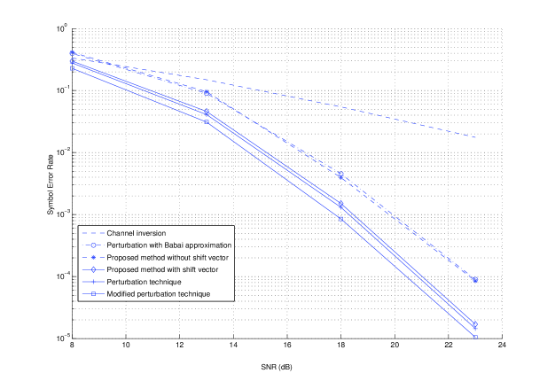
Figure 2: Symbol Error Rate of the proposed schemes, the perturbation scheme [1], and the naive channel inversion approach for $N_{t}=4$ transmit antennas and $N_{r}=4$ single-antenna receivers with the rate $R=2$ bits per channel use per user.

Figure 3 compares the regularized proposed scheme with V-BLAST modifications of Zero-Forcing and Babai approximation for the same setting. As shown in the simulation results (and also in the simulation results in [1] and [14]), the modulo-MMSE-VBLAST scheme does not achieve a precoding diversity better than zero forcing (though it has a good performance in the low SNR region). However, combining the lattice-reduction-aided (LRA) scheme with MMSE-VBLAST precoding or other schemes such as regularization improves its performance by a finite coding gain (without changing the slope of the curve of symbol-error-rate). Combining both the regularization and the shift vector can result in better performance compared to other alternatives.

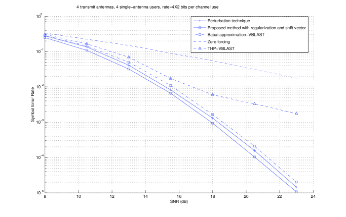
Figure 3: Comparison of the regularized proposed scheme with V-BLAST modifications of Zero-Forcing and Babai approximation (for $N_{t}=4$ transmit antennas and $N_{r}=4$ single-antenna receivers with the rate $R=2$ bits per channel use per user.).

Figure 4 compares the performances of the fixed-rate and the variable-rate transmission using lattice-basis reduction for $N_{t}=2$ transmit antennas and $N_{r}=2$ users. In both cases, the sum-rate is 8 bits per channel use (in the case of fixed individual rates, a 16QAM constellation is assigned to each user). We see that by eliminating the equal-rate constraint, we can considerably improve the performance (especially, for high rates). In fact, the diversity gains for the equal-rate and the unequal-rate methods are, respectively, $N_{r}$ and $N_{t}N_{r}$.

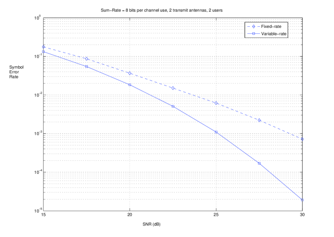
Figure 4: Performance comparison between the fixed-rate and the variable-rate transmission for $N_{t}=2$ transmit antennas and $N_{r}=2$ single-antenna receivers with sum-rate 8 bits per channel use.

VIII Conclusion

A simple scheme for communications in MIMO broadcast channels is introduced which is based on the lattice reduction technique and improves the performance of the channel inversion method. Lattice basis reduction helps us to reduce the average transmitted energy by modifying the region which includes the constellation points. Simulation results show that the performance of the proposed scheme is very close to the performance of the perturbation method. Also, it is shown that by using lattice-basis reduction, we achieve the maximum precoding diversity with a polynomial-time precoding complexity.

Appendix A

In this Appendix, we compute the second moment of a parallelotope whose centroid is the origin and its edges are equal to the basis vectors of the lattice.

Assume that $\cal A$ is an $M$-dimensional parallelotope and $X$ is its second moment. The second moment of $\frac{1}{2}\cal A$ is $\left(\frac{1}{2}\right)^{M+2}X$. The parallelotope $\cal A$ can be considered as the union of $2^{M}$ smaller parallelotopes which are constructed by $\pm\frac{1}{2}\mathbf{b}_{1},\pm\frac{1}{2}\mathbf{b}_{2},....,\pm\frac{1}{2}\mathbf{b}_{M}$, where $\mathbf{b}_{i}$, $1\leq i\leq M$, is a basis vector. These parallelotopes are translated versions of $\frac{1}{2}\cal A$ with the translation vectors $T_{i}=\pm\frac{1}{2}\mathbf{b}_{1}\pm\frac{1}{2}\mathbf{b}_{2}\pm....\pm\frac{1}{2}\mathbf{b}_{M}$, $1\leq i\leq 2^{M}$. The second moments of these parallelotopes are equal to $\left(\frac{1}{2}\right)^{M+2}X+\|T_{i}\|^{2}\mbox{Vol}(\frac{1}{2}{\cal A})$, $1\leq i\leq 2^{M}$. By the summation over all these second moments, we can find the second moment of $\cal A$.

$$X=\sum_{i=1}^{2^{M}}\left[\left(\frac{1}{2}\right)^{M+2}X+\|T_{i}\|^{2}.\mbox{Vol}(\frac{1}{2}{\cal A})\right]$$ (100)

$$=\left(\frac{1}{2}\right)^{2}X+2^{M-2}(\|\mathbf{b}_{1}\|^{2}+...+\|\mathbf{b}_{M}\|^{2}).\mbox{Vol}(\frac{1}{2}{\cal A})$$ (101)

$$=\frac{1}{4}X+\frac{1}{4}(\|\mathbf{b}_{1}\|^{2}+...+\|\mathbf{b}_{M}\|^{2}).\mbox{Vol}({\cal A})$$ (102)

$$\Longrightarrow X=\frac{1}{3}(\|\mathbf{b}_{1}\|^{2}+...+\|\mathbf{b}_{M}\|^{2}).\mbox{Vol}({\cal A}).$$ (103)

Appendix B

Proof of Lemma 3

Lemma 3 states that the probability that a lattice, generated by $M$ independent $N$-dimensional complex Gaussian vectors, $N\geq M$, with a unit variance per each dimension, has a nonzero point inside a sphere (centered at origin and with the radius $\varepsilon$) is bounded by $\beta_{N,M}\varepsilon^{2N}$ for $N>M$, and $\beta_{N,M}\varepsilon^{2N}\max\left\{(-\ln\varepsilon)^{N+1},1\right\}$ for $N=M\geq 2$. We can assume that $\varepsilon<1$ (for $\varepsilon\geq 1$, lemma 3 is trivial because the probability is bounded).

VIII-A Case 1: $M=1$

When $M=1$, the lattice consists of the integer multiples of the basis vector $\mathbf{v}$. If the norm of one of these vectors is less than $\varepsilon$, then the norm of $\mathbf{v}$ is less than $\varepsilon$. Consider the variance of the components of $\mathbf{v}$ as $\varrho^{2}$. The vector $\mathbf{v}$ has an $N$-dimensional complex Gaussian distribution, $f_{\mathbf{v}}(\mathbf{v})$. Therefore, the probability of this event is,

$$\Pr\left\{\|\mathbf{v}\|\leq\varepsilon\right\}=\int_{\|\mathbf{v}\|\leq\varepsilon}f_{\mathbf{v}}(\mathbf{v})\;d\mathbf{v}\leq\int_{\|\mathbf{v}\|\leq\varepsilon}\frac{1}{\pi^{N}\varrho^{2N}}\;d\mathbf{v}\leq\beta_{N,1}\frac{\varepsilon^{2N}}{\varrho^{2N}}.$$ (104)

When the variance of the components of $\mathbf{v}$ is equal to one, we have,

$$\Pr\left\{\|\mathbf{v}\|\leq\varepsilon\right\}\leq\beta_{N,1}\varepsilon^{2N}.$$ (105)

VIII-B Case 2: $N>M>1$

Consider $L_{(\mathbf{v}_{1},...,\mathbf{v}_{M})}$ as the lattice generated by $\mathbf{v}_{1}$,$\mathbf{v}_{2}$,…,$\mathbf{v}_{M}$. Each point of $L_{(\mathbf{v}_{1},...,\mathbf{v}_{M})}$ can be represented by $\mathbf{v}_{(z_{1},...,z_{M})}=z_{1}\mathbf{v}_{1}+z_{2}\mathbf{v}_{2}+...+z_{M}\mathbf{v}_{M}$, where $z_{1},...,z_{M}$ are complex integer numbers. The vectors $\mathbf{v}_{1}$,$\mathbf{v}_{2}$,…,$\mathbf{v}_{M}$ are independent and jointly Gaussian. Therefore, for every integer vector $\mathbf{z}=(z_{1},...,z_{M})$, the entries of the vector $\mathbf{v}_{(z_{1},...,z_{M})}$ have complex Gaussian distributions with the variance

$$\varrho_{\mathbf{z}}^{2}=\|\mathbf{z}\|^{2}\varrho^{2}=\left(|z_{1}|^{2}+...+|z_{M}|^{2}\right)\varrho^{2}.$$ (106)

Therefore, according to the lemma for $M=1$,

$$\Pr\left\{\|\mathbf{v}_{(z_{1},...,z_{M})}\|\leq\varepsilon\right\}\leq\beta_{N,1}\frac{\varepsilon^{2N}}{\left(|z_{1}|^{2}+...+|z_{M}|^{2}\right)^{N}}.$$ (107)

Now, by using the union bound,

$$\Pr\left\{d_{\mathbf{H}}\leq\varepsilon\right\}\leq\sum_{\mathbf{z}\neq 0}\Pr\left\{\|\mathbf{v}_{(z_{1},...,z_{M})}\|\leq\varepsilon\right\}$$ (108)

$$\leq\sum_{\mathbf{z}\neq 0}\beta_{N,1}\frac{\varepsilon^{2N}}{\left(|z_{1}|^{2}+...+|z_{M}|^{2}\right)^{N}}$$ (109)

$$=\beta_{N,1}\left(\sum_{1\leq\|\mathbf{z}\|<2}\frac{\varepsilon^{2N}}{\|\mathbf{z}\|^{2N}}+\sum_{2\leq\|\mathbf{z}\|<3}\frac{\varepsilon^{2N}}{\|\mathbf{z}\|^{2N}}\right.$$

$$\left.+\sum_{3\leq\|\mathbf{z}\|<4}\frac{\varepsilon^{2N}}{\|\mathbf{z}\|^{2N}}+...\right).$$ (110)

The $M$-dimensional complex integer points $\mathbf{z}=(z_{1},...,z_{M})$, such that $k\leq\|\mathbf{z}\|<k+1$, can be considered as the centers of disjoint unit-volume cubes. All these cubes are inside the region between the $2M$-dimensional spheres, with radii $k-1$ and $k+2$. Therefore, the number of $M$-dimensional complex integer points $\mathbf{z}=(z_{1},...,z_{M})$, such that $k\leq\|\mathbf{z}\|<k+1$, can be bounded by the volume of the region between these two $2M$-dimensional spheres. Thus, this number is bounded by $c_{1}k^{2M-1}$ for some constant $c_{1}$. Therefore,

$$\sum_{k\leq\|\mathbf{z}\|<k+1}\frac{\varepsilon^{2N}}{\|\mathbf{z}\|^{2N}}\leq c_{1}k^{2M-1}\frac{\varepsilon^{2N}}{k^{2N}}$$ (111)

$${\rm(\ref{eq:92}),(\ref{eq:95})}\Longrightarrow\Pr\left\{d_{\mathbf{H}}\leq\varepsilon\right\}\leq c_{1}\beta_{N,1}\varepsilon^{2N}+2^{2M-1}c_{1}\beta_{N,1}\frac{\varepsilon^{2N}}{2^{2N}}+$$

$$+3^{2M-1}c_{1}\beta_{N,1}\frac{\varepsilon^{2N}}{3^{2N}}+...$$ (112)

$$\leq c_{1}\beta_{N,1}\varepsilon^{2N}\sum_{k=1}^{\infty}\frac{1}{k^{2N-2M+1}}.$$ (113)

According to the assumption of this case, $N>M$; hence, $2N-2M+1\geq 2$. Therefore, the above summation is convergent:

$$\Pr\left\{\|\mathbf{v}\|\leq\varepsilon\right\}\leq\beta_{N,M}\varepsilon^{2N}.$$ (114)

VIII-C Case 3: $N=M>1$

Each point of $L_{(\mathbf{v}_{1},...,\mathbf{v}_{N})}$ can be represented by $z\mathbf{v}_{N}-\mathbf{v}$, where $\mathbf{v}$ belongs to the lattice $L_{(\mathbf{v}_{1},...,\mathbf{v}_{N-1})}$ and $z$ is a complex integer. Consider $\mathcal{S}_{\mathbf{v}}$ as the sphere with radius $\varepsilon$ and centered at ${\mathbf{v}}$. Now, $z\mathbf{v}_{N}-\mathbf{v}$ belongs to $\mathcal{S}_{\mathbf{0}}$ iff the $z\mathbf{v}_{N}$ belongs to $\mathcal{S}_{\mathbf{v}}$. Also, the sphere $\mathcal{S}_{\mathbf{v}}$ includes a point $z\mathbf{v}_{N}$ iff $\mathcal{S}_{\mathbf{v},z}$ includes $\mathbf{v}$ , where $\mathcal{S}_{\mathbf{v},z}=\frac{\mathcal{S}_{\mathbf{v}}}{z}$ is the sphere centered at $\mathbf{v}/z$ with radius $\dfrac{\varepsilon}{|z|}$ (see figure 4). Therefore, the probability that a lattice point exists in $\mathcal{S}_{\mathbf{v}}$ is equal to the probability that $\mathbf{v}_{N}$ is in at least one of the spheres $\left\{\mathcal{S}_{\mathbf{v},z}\right\}$, $z\neq 0$.

Figure 5: The family of spheres ${\mathcal{S}_{\mathbf{v},z}}$

If we consider $d_{\mathbf{H}}$ as the minimum distance of $L_{(\mathbf{v}_{1},...,\mathbf{v}_{N})}$ and $R$ as an arbitrary number greater than 1:

$$\Pr\left\{d_{\mathbf{H}}\leq\varepsilon\right\}=\Pr\left\{\left(L_{(\mathbf{v}_{1},...,\mathbf{v}_{N})}-0\right)\cap\mathcal{S}_{\mathbf{0}}\neq\varnothing\right\}=\Pr\left\{\mathbf{v}_{N}\in\bigcup_{\mathbf{v}}\bigcup_{z\neq 0}\mathcal{S}_{\mathbf{v},z}\right\}$$ (115)

$$\leq\Pr\left\{\mathbf{v}_{N}\in\bigcup_{\|\frac{\mathbf{v}}{z}\|\leq R}\mathcal{S}_{\mathbf{v},z}\right\}+\Pr\left\{\mathbf{v}_{N}\in\bigcup_{\|\frac{\mathbf{v}}{z}\|>R}\mathcal{S}_{\mathbf{v},z}\right\}$$ (116)

In the second term of (116), all the spheres have centers with norms greater than $R$ and radii less than 1 (because $|z|\geq 1$). Therefore,

$$\bigcup_{\|\frac{\mathbf{v}}{z}\|>R}\mathcal{S}_{\mathbf{v},z}\subset\left\{\mathbf{x}\left|\right.\|\mathbf{x}\|>R-1\right\}$$ (117)

$${\rm(\ref{eq:102})}\Longrightarrow{\rm(\ref{eq:101})}\leq\Pr\left\{\mathbf{v}_{N}\in\bigcup_{\|\frac{\mathbf{v}}{z}\|\leq R}\mathcal{S}_{\mathbf{v},z}\right\}+\Pr\left\{\|\mathbf{v}_{N}\|>R-1\right\}$$ (118)

$$\leq\Pr\left\{\mathbf{v}_{N}\in\bigcup_{\|\frac{\mathbf{v}}{z}\|\leq R,|z|\leq\varepsilon^{1-N}}\mathcal{S}_{\mathbf{v},z}\right\}+\Pr\left\{\mathbf{v}_{N}\in\bigcup_{\|\frac{\mathbf{v}}{z}\|\leq R,|z|>\varepsilon^{1-N}}\mathcal{S}_{\mathbf{v},z}\right\}+\Pr\left\{\|\mathbf{v}_{N}\|>R-1\right\}.$$ (119)

We bound the first term of (119) as the following:

$$\Pr\{\mathbf{v}_{N}\in\bigcup_{\|\frac{\mathbf{v}}{z}\|\leq R,|z|\leq\varepsilon^{1-N}}\mathcal{S}_{\mathbf{v},z}\}$$ (120)

$$\leq\left(\sum_{\|\mathbf{v}\|\leq 2R}\sum_{|z|\geq 1}\Pr\{\mathbf{v}_{N}\in\mathcal{S}_{\mathbf{v},z}\}+\sum_{2R<\|\mathbf{v}\|\leq 3R}\sum_{|z|\geq 2}\Pr\{\mathbf{v}_{N}\in\mathcal{S}_{\mathbf{v},z}\}+\right.$$

$$\left....+\sum_{\lfloor\varepsilon^{1-N}\rfloor R<\|\mathbf{v}\|\leq(\lfloor\varepsilon^{1-N}\rfloor+1)R}\;\;\;\sum_{|z|\geq\lfloor\varepsilon^{1-N}\rfloor}\Pr\{\mathbf{v}_{N}\in\mathcal{S}_{\mathbf{v},z}\}\right).$$ (121)

Noting that the pdf of $\mathbf{v}_{N}$ is less than or equal to $\frac{1}{\pi^{N}}$,

$${\rm(\ref{eq:105})}\leq\frac{1}{\pi^{N}}\left(\sum_{\|\mathbf{v}\|\leq 2R}\sum_{|z|\geq 1}{\rm Vol}(\mathcal{S}_{\mathbf{v},z})+\sum_{2R<\|\mathbf{v}\|\leq 3R}\sum_{|z|\geq 2}{\rm Vol}(\mathcal{S}_{\mathbf{v},z})+\right.$$

$$\left....+\sum_{\lfloor\varepsilon^{1-N}\rfloor R<\|\mathbf{v}\|\leq(\lfloor\varepsilon^{1-N}\rfloor+1)R}\;\;\;\sum_{|z|\geq\lfloor\varepsilon^{1-N}\rfloor}{\rm Vol}(\mathcal{S}_{\mathbf{v},z})\right)$$ (122)

$$\leq\frac{1}{\pi^{N}}\left(\sum_{\|\mathbf{v}\|\leq 2R}\sum_{|z|\geq 1}\frac{c_{2}\varepsilon^{2N}}{|z|^{2N}}+\sum_{2R<\|\mathbf{v}\|\leq 3R}\sum_{|z|\geq 2}\frac{c_{2}\varepsilon^{2N}}{|z|^{2N}}+\right.$$

$$\left....+\sum_{\lfloor\varepsilon^{1-N}\rfloor R<\|\mathbf{v}\|\leq(\lfloor\varepsilon^{1-N}\rfloor+1)R}\;\;\;\sum_{|z|\geq\lfloor\varepsilon^{1-N}\rfloor}\frac{c_{2}\varepsilon^{2N}}{|z|^{2N}}\right).$$ (123)

By using (111), for one-dimensional complex vector $\mathbf{z}=z$,

$$\sum_{|z|\geq i}\frac{c_{2}\varepsilon^{2N}}{|z|^{2N}}=\sum_{k=i}^{\infty}c_{2}.\sum_{k\leq|z|\leq k+1}\frac{\varepsilon^{2N}}{|z|^{2N}}\leq\sum_{k=i}^{\infty}\frac{c_{1}c_{2}\varepsilon^{2N}}{k^{2N-1}}\leq\frac{c_{3}\varepsilon^{2N}}{i^{2N-2}}$$ (124)

Now,

$${\rm(\ref{eq:110})}\Longrightarrow{\rm(\ref{eq:105})}\leq\frac{1}{\pi^{N}}\left(\sum_{\|\mathbf{v}\|\leq 2R}c_{3}\varepsilon^{2N}+\sum_{2R<\|\mathbf{v}\|\leq 3R}\frac{c_{3}\varepsilon^{2N}}{2^{2N-2}}+\right.$$

$$\left....+\sum_{\lfloor\varepsilon^{1-N}\rfloor R<\|\mathbf{v}\|\leq(\lfloor\varepsilon^{1-N}\rfloor+1)R}\frac{c_{3}\varepsilon^{2N}}{\lfloor\varepsilon^{1-N}\rfloor^{2N-2}}\right).$$ (125)

Assume that the minimum distance of $L_{(\mathbf{v}_{1},...,\mathbf{v}_{N-1})}$ is $d_{N-1}$. The spheres with the radius $d_{N-1}/2$ and centered by the points of $L_{(\mathbf{v}_{1},...,\mathbf{v}_{N-1})}$ are disjoint. Therefore, the number of points from the ($N-1$)-dimensional complex lattice $L_{(\mathbf{v}_{1},...,\mathbf{v}_{N-1})}$, such that $\|\mathbf{v}\|\leq 2R$, is bounded by $\frac{c_{4}(2R+d_{N-1}/2)^{2N-2}}{d_{N-1}^{2N-2}}$ (it is bounded by the ratio between the volumes of ($2N-2$)-dimensional spheres with radii $2R+d_{N-1}/2$ and $d_{N-1}/2$). Also, the number of points from $L_{(\mathbf{v}_{1},...,\mathbf{v}_{N-1})}$, such that $(k-1)R<\|\mathbf{v}\|\leq kR$, is bounded by $\frac{c_{4}(kR)^{2N-3}(R+d_{N-1})}{d_{N-1}^{2N-2}}$ (it is bounded by the ratio between the volumes of the region defined by $(k-1)R-d_{N-1}/2<\|\mathbf{x}\|\leq kR+d_{N-1}/2$ and the sphere with radius $d_{N-1}/2$):

$$(\ref{eq:153})\leq\frac{c_{5}(2R+d_{N-1}/2)^{2N-2}}{d_{N-1}^{2N-2}}.\varepsilon^{2N}+\frac{c_{5}R^{2N-3}(R+d_{N-1})}{d_{N-1}^{2N-2}}.\varepsilon^{2N}\sum_{k=2}^{\lfloor\varepsilon^{1-N}\rfloor}\frac{1}{k}$$ (126)

$$(\ref{eq:153})\leq\frac{c_{5}(2R+d_{N-1}/2)^{2N-2}}{d_{N-1}^{2N-2}}.\varepsilon^{2N}+\frac{c_{5}R^{2N-3}(R+d_{N-1})}{d_{N-1}^{2N-2}}.\varepsilon^{2N}.\ln(\varepsilon^{1-N})$$ (127)

$$\leq c_{6}\varepsilon^{2N}.\max\left(\frac{R^{2N-2}}{d_{N-1}^{2N-2}},1\right).\max\left\{-\ln\varepsilon,1\right\}.$$ (128)

According to the proof of the case 2, we have $\Pr\left\{d_{N-1}\leq\eta\right\}\leq\beta_{N,N-1}\eta^{2N}$. Therefore,

$${\rm E}_{d_{N-1}}\left\{\max\left(\frac{R^{2N-2}}{d_{N-1}^{2N-2}},1\right)\right\}$$ (129)

$$\leq 1.\Pr\left\{d_{N-1}>R\right\}+2^{2N-2}.\Pr\left\{\frac{1}{2}R<d_{N-1}\leq R\right\}+3^{2N-2}.\Pr\left\{\frac{1}{3}R<d_{N-1}\leq\frac{1}{2}R\right\}+...$$ (130)

$$\leq 1+2^{2N-2}.\Pr\left\{d_{N-1}\leq R\right\}+3^{2N-2}.\Pr\left\{d_{N-1}\leq\frac{1}{2}R\right\}+...$$ (131)

$$\leq 1+\sum_{k=1}^{\infty}\frac{(k+1)^{2N-2}}{k^{2N}}.R^{2N}\beta_{N,N-1}\leq c_{7}R^{2N}$$ (132)

$$\Longrightarrow{\rm E}_{d_{N-1}}\left\{c_{6}\varepsilon^{2N}.\max\left(\frac{R^{2N-2}}{d_{N-1}^{2N-2}},1\right).\max\left\{-\ln\varepsilon,1\right\}\right\}\leq c_{8}\varepsilon^{2N}.R^{2N}.\max\left\{-\ln\varepsilon,1\right\}.$$ (133)

To bound the second term of (119), we note that for $|z|\geq\varepsilon^{1-N}$, the radii of the spheres $\mathcal{S}_{\mathbf{v},z}$ are less or equal to $\varepsilon^{N}$, and the centers of these spheres lie on the $(N-1)$-dimensional complex subspace containing $L_{\mathbf{v}_{1},...,\mathbf{v}_{N-1}}$. Also, the norm of these centers are less than $R$. Therefore, all of these spheres are inside the region $\mathcal{A}$ which is an orthotope centered at the origin, with $2N$ real dimensions (see figure 5):

$$\bigcup_{\|\frac{\mathbf{v}}{z}\|\leq R,|z|>\varepsilon^{1-N}}\mathcal{S}_{\mathbf{v},z}\subset\mathcal{A}$$ (134)

$$\Longrightarrow\Pr\{\mathbf{v}_{N}\in\bigcup_{\|\frac{\mathbf{v}}{z}\|\leq R,|z|>\varepsilon^{1-N}}\mathcal{S}_{\mathbf{v},z}\}\leq\frac{1}{\pi^{N}}{\rm Vol}\left(\bigcup_{\|\frac{\mathbf{v}}{z}\|\leq R,|z|>\varepsilon^{1-N}}\mathcal{S}_{\mathbf{v},z}\right)\leq\frac{1}{\pi^{N}}{\rm Vol}(\mathcal{A})$$ (135)

$$\leq\frac{1}{\pi^{N}}(2\varepsilon^{N})^{2}(2R+\varepsilon^{N})^{2N-2}$$ (136)

Figure 6: The orthotope $\mathcal{A}$

Also, according to the Gaussian distribution of the entries of $\mathbf{v}_{N}$ (which have Variance $\frac{1}{2}$ on each real dimension), we can bound the third term of (119) as,

$$\Pr\{\|\mathbf{v}_{N}\|>R-1\}\leq 2NQ\left(\sqrt{\frac{R-1}{N}}\right)\leq c_{9}e^{-\left(\frac{R-1}{\sqrt{2}N}\right)^{2}}.$$ (137)

By using (133), (136), and (137),

$$\Pr\left\{d_{\mathbf{H}}\leq\varepsilon\right\}\leq c_{8}\varepsilon^{2N}.R^{2N}.\max\left\{-\ln\varepsilon,1\right\}+\frac{1}{\pi^{N}}(2\varepsilon^{N})^{2}(2R+\varepsilon^{N})^{2N-2}+c_{9}e^{-\left(\frac{R-1}{\sqrt{2}N}\right)^{2}}.$$ (138)

The above equation is true for every $R>1$. Therefore, using $R=\sqrt{2}N\sqrt{-\ln(\varepsilon^{2N})}+1$,

$$\Pr\left\{d_{\mathbf{H}}\leq\varepsilon\right\}\leq\beta_{N,N}\varepsilon^{2N}.\max\left\{(-\ln\varepsilon)^{N+1},1\right\}.$$ (139)

References

• [1] C. B. Peel, B. M. Hochwald, and A. L. Swindlehurst, “A vector-perturbation technique for near-capacity multiple-antenna multi-user communications-Part II: Perturbation,” IEEE Trans. Comm., pp. 537 – 544, March 2005.
• [2] I. E. Telatar, “Capacity of multi-antenna gaussian channels,” Europ. Trans. Telecommun., pp. 585–595, Nov. 1999.
• [3] G. J. Foschini, “Layered space-time architechture for wireless communication in a fading environment when using multi-element antennas,” Bell labs. Tech. J., vol. 1, no. 2, pp. 41–59, 1996.
• [4] V. Tarokh, N. Seshadri, and A. R. Calderbank, “Space-time codes for high data rate wireless communication: Performance criterion and code construction,” IEEE Trans. Info. Theory, vol. 44, pp. 744–765, Mar. 1998.
• [5] V. Tarokh, H. Jafarkhani, and A. R. Calderbank, “Space-time block codes from orthogonal designs,” IEEE Trans. Info. Theory, vol. 45, pp. 1456–1467, July 1999.
• [6] S. M. Alamouti, “A simple transmitter diversity scheme for wireless communications,” IEEE J. Selec. Areas Commun., vol. 16, pp. 1451–1458, Oct. 1998.
• [7] G. Caire and S. Shamai, “On the acheivable throughput of a multiple-antenna Gaussian broadcast channel,” IEEE Trans. Info. Theory, pp. 1691–1706, July 2003.
• [8] W. Yu and J. Cioffi, “Sum capacity of a Gaussian vector broadcast channel,” in Proceedings IEEE International Symposium on Information Theory, p. 498, 2002.
• [9] P. Viswanath and D. Tse, “Sum capacity of the vector Gaussian broadcast channel and uplink-downlink duality,” IEEE Trans. Info Theory, pp. 1912–1921, August 2003.
• [10] S. Vishwanath, N. Jindal, and A. Goldsmith, “Duality, acheivable rates and sum capacity of Gaussian MIMO broadcast channels,” IEEE Trans. Info. Theory, pp. 2658–2658, August 2003.
• [11] M. Costa, “Writing on dirty paper,” IEEE Trans. Info. Theory, vol. 29, pp. 439–441, May 1983.
• [12] U. Erez, S. Shamai, and R. Zamir, “Capacity and lattice strategies for canceling known interference,” IEEE Trans. Info. Theory, pp. 3820 – 3833, Nov. 2005.
• [13] C. Windpassinger and R. Fischer, “Low-complexity near-maximum-likelihood detection and precoding for MIMO systems using lattice reduction,” in Proceedings of Information Theory Workshop, 2003.
• [14] C. Windpassinger, R. F. H. Fischer, and J. B. Huber, “Lattice-reduction-aided broadcast precoding,” in 5th International ITG Conference on Source and Channel Coding (SCC), (Erlangen, Germany), pp. 403–408, January 2004.
• [15] C. Windpassinger, R. Fischer, and J. B. Huber, “Lattice-reduction-aided broadcast precoding,” IEEE Trans. Communications, pp. 2057–2060, Dec. 2004.
• [16] R. Fischer, “Lattice-reduction-aided equalization and generalized partial response signaling for point-to-point transmission over flat-fading MIMO channels,” in 6th International ITG-Conference on Source and Channel Coding, (Munich, Germany), April 2006.
• [17] M. Grotschel, L. Lovasz, and A. Schrijver, Geometrical algorithms and combinatorial optimization, ch. 5. Springer-Verlag, 1993.
• [18] P. M. Gruber and C. G. Lekkerkerker, Geometry of numbers. North-Holland, 1987.
• [19] B. Helfrich, “Algorithms to construct minkowski reduced and hermit reduced lattice bases,” Theoretical Computer Sci. 41, pp. 125–139, 1985.
• [20] A. K. Lenstra, H. W. Lenstra, and L. Lovasz, “Factoring polynomials with rational coefficients,” Mathematische Annalen, vol. 261, pp. 515–534, 1982.
• [21] H. Napias, “A generalization of the LLL algorithm over euclidean rings or orders,” Journal de théorie des nombres de Bordeaux, vol. 8, pp. 387–396, 1996.
• [22] G. D. Forney and L. F. Wei, “Multidimensional constellations-Part I: Introduction, figures of merit, and generalized cross constellations,” IEEE J. Select Areas Commun., vol. 7, pp. 877–892, August 1989.
• [23] M. Ajtai, “The shortest vector problem in L2 is NP-hard for randomized reductions,” in Proceedings of the thirtieth annual ACM symposium on Theory of computing, pp. 10–19, 1998.
• [24] J. H. Conway and N. J. A. Sloane, Sphere packing, lattices and groups. Springer-Verlag, 1999.
• [25] C. B. Peel, B. M. Hochwald, and A. L. Swindlehurst, “A vector-perturbation technique for near-capacity multiple-antenna multi-user communications-Part I: channel inversion and regularization,” IEEE Trans. Comm., pp. 195 – 202, Jan. 2005.
• [26] D. A. Schmidt, M. Joham, and W. Utschick, “Minimum mean square error vector precoding,” in PIMRC 2005, pp. 107–111, 2005.
• [27] E. Agrell, T. Eriksson, A. Vardy, , and K. Zeger, “Closest point search in lattices,” IEEE Trans. Info. Theory, vol. 48, pp. 2201–2214, August 2002.
• [28] L. Zheng and D. Tse, “Diversity and multiplexing: a fundamental tradeoff in multiple-antenna channels,” IEEE Trans. Info. Theory, pp. 1073–1096, May 2003.
• [29] M. Markus and H. Minc, A survey of matrix theory and matrix inequalities. Dover, 1964.