Gaussian Channels with Feedback: Optimality, Fundamental Limitations, and Connections of Communication, Estimation, and Control

Abstract

Gaussian channels with memory and with noiseless feedback have been widely studied in the information theory literature. However, a coding scheme to achieve the feedback capacity is not available. In this paper, a coding scheme is proposed to achieve the feedback capacity for Gaussian channels. The coding scheme essentially implements the celebrated Kalman filter algorithm, and is equivalent to an estimation system over the same channel without feedback. It reveals that the achievable information rate of the feedback communication system can be alternatively given by the decay rate of the Cramer-Rao bound of the associated estimation system. Thus, combined with the control theoretic characterizations of feedback communication (proposed by Elia), this implies that the fundamental limitations in feedback communication, estimation, and control coincide. This leads to a unifying perspective that integrates information, estimation, and control. We also establish the optimality of the Kalman filtering in the sense of information transmission, a supplement to the optimality of Kalman filtering in the sense of information processing proposed by Mitter and Newton. In addition, the proposed coding scheme generalizes the Schalkwijk-Kailath codes and reduces the coding complexity and coding delay. The construction of the coding scheme amounts to solving a finite-dimensional optimization problem. A simplification to the optimal stationary input distribution developed by Yang, Kavcic, and Tatikonda is also obtained. The results are verified in a numerical example.

I Introduction

Communication systems in which the transmitters have access to noiseless feedback of channel outputs have been widely studied. As one of the most important case, the single-input single-output frequency-selective Gaussian channels with feedback have attracted considerable attention; see [1, 2, 3, 4, 5, 6, 7, 8, 9, 10, 11, 12, 13, 14, 15, 16] and references therein for the capacity computation and coding scheme design for these channels. In particular, [1, 2] proposed ingenious feedback codes (called the Schalkwijk-Kailath codes, in short the SK codes) for additive white Gaussian noise (AWGN) channels, which achieve the asymptotic feedback capacity (i.e. the infinite-horizon feedback capacity, denoted $C_{\infty}$) and greatly reduce the coding complexity and coding delay. [4, 5, 7] presented the extensions of the SK codes to Gaussian feedback channels with memory and obtained tight capacity bounds.

[6] presented a rather general coding structure (called the Cover-Pombra structure, in short the CP structure) to achieve the finite-horizon feedback capacity (denoted $C_{T}$, where the horizon spans from time epoch 0 to time epoch $T$) for Gaussian channels with memory; however, it involves prohibitive computation complexity as the coding length $(T+1)$ increases. By exploiting the special properties of a moving-average Gaussian channel with feedback, [9] discovered the finite rankness of the innovations in the CP structure, which reduces the computation complexity. [10] reformulated the CP structure along this direction, and obtained an SK-based coding scheme to achieve $C_{T}$ with reduced computation complexity. Also along the line of [9], [15] studied a first-order moving-average Gaussian channel with feedback, found the closed-form expression for $C_{\infty}$, and obtained an SK-based coding scheme to achieve $C_{\infty}$.

[11] provided a thorough study of feedback capacity; extended the notion of directed information proposed in [17] and proved that its supremum is the feedback capacity; reformulated the problem of computing $C_{T}$ as a stochastic control optimization problem; and proposed a dynamic programming based solution. This idea was further explored in [12], which uncovered the Markov property of the optimal input distributions for Gaussian channels with memory and eventually reduced the finite-horizon stochastic control optimization problem to a manageable size. Moreover, under a stationarity conjecture that $C_{\infty}$ equals the stationary capacity (the maximum information rate over all stationary input distributions, denoted $C^{s}$), $C_{\infty}$ is given by the solution of a finite dimensional optimization problem. This is the first computationally efficient method to calculate $C^{s}$ or $C_{T}$ for general Gaussian channels. The stationary conjecture has been recently confirmed, namely $C^{s}=C_{\infty}$, and $C_{\infty}$ is achievable using a (an asymptotically) stationary input distribution [16].

[3] proposed a view of regarding the optimal communication over an AWGN channel with feedback as a control problem. [13] investigated the problem of tracking unstable sources over a channel and introduced the notion of anytime capacity to capture the fundamental limitations in that problem, which reveals intimate connections between communication and control and brings new insights to feedback communication problems. Furthermore, [14] established the equivalence between feedback communication and feedback stabilization over Gaussian channels with memory, showed that the achievable transmission rate is given by the Bode sensitivity integral of the associated control system, and presented an optimization problem based on robust control to compute lower bounds of $C^{s}$. [14] also extended the SK codes to achieve these lower bounds, and the coding schemes have an interpretation of tracking unstable sources over Gaussian channels.

For Gaussian networks with feedback, tight capacity bounds can be found in [18, 19, 14]. For time-selective fading channels with AWGN and with feedback, an SK-based coding scheme utilizing the channel fading information was constructed in [20] to achieve the ergodic capacity.

As we can see, it remains an open problem to build a coding scheme with reasonable complexity to achieve $C_{\infty}$ for a Gaussian channel with memory; note that no practical codes have been found based on the optimal signalling strategy in [12]. In this paper, we propose a coding scheme for frequency-selective Gaussian channels with output feedback. This coding scheme achieves $C_{\infty}$, the asymptotic feedback capacity of the channel; utilizes the Kalman filter algorithm; simplifies the coding processes; and shortens the coding delay. The optimal coding structure is essentially a finite-dimensional linear time-invariant (FDLTI) system, is also an extension of the SK codes, and leads to a further simplification of the optimal stationary signalling strategy in [12]. The construction of the coding system amounts to solving a finite-dimensional optimization problem. Our solution holds for AWGN channels with intersymbol interference (ISI) where the ISI is model as a stable and minimum-phase FDLTI system; through the equivalence shown in [11, 12], this channel is equivalent to a colored Gaussian channel with rational noise power spectrums and without ISI. Note that the rationalness assumption is widely used and not too restrictive, since any power spectrum can be arbitrarily approximated by rational ones.

In deriving our optimal coding design in infinite-horizon, we first present finite-horizon analysis (which is closely related to the CP structure) of the feedback communication problem, and then let the horizon length tend to infinity and obtain our optimal coding design which achieves $C_{\infty}$. More specifically, in our finite-horizon analysis, we establish the necessity of the Kalman filter: The Kalman filter is not only a device to provide sufficient statistics (which was shown in [12]), but also a device to ensure the power efficiency and to recover the message optimally. This also leads to a refinement of the CP structure, applicable for generic Gaussian channels. Additionally, the presence of the Kalman filter in our coding scheme reveals the intrinsic connections among feedback communication, estimation, and control. In particular, we show that the feedback communication problem over a Gaussian channel is essentially an optimal estimation problem, and the achievable rate of the feedback communication system is alternatively given by the decay rate of the Cramer-Rao bound (CRB) for the associated estimation system. Invoking the Bode sensitivity characterization of the achievable rate [14], we conclude that the fundamental limitations in feedback communication, estimation, and control coincide. We then extend the horizon to infinity and characterize the steady-state of the feedback communication problem. We finally show that our optimal scheme achieves $C_{\infty}$.

We also remark that the necessity of the Kalman filter in the optimal coding scheme is not surprising, given various indications of the essential role of Kalman filtering (or minimum mean-squared error (MMSE) estimators; or minimum-energy control, its control theory equivalence; or the sum-product algorithm, its generalization) in optimal communication designs. See e.g. [21, 22, 23, 12, 14, 24]. The study of the Kalman filter in the feedback communication problem along the line of [24] may shed important insights on optimal communication problems and is under current investigation.

One main insight gained in this study is that, the perspective of unifying information, estimation, and control, three fundamental concepts, facilitates our development of the optimal feedback communication design. Though the connections between any two of the three concepts have been investigated or are under investigation, a joint study explicitly addressing all three is not available. Our study provides the first example that the connections among the three can be explored and utilized, to the best of our knowledge. In addition to helping us to achieve the optimality in the feedback communication problem, this new perspective establishes the optimality of the Kalman filtering in the sense of information transmission, a supplement to the optimality of Kalman filtering in the sense of information processing proposed by Mitter and Newton [24]. It also leads to a new formula connecting the mutual information in the feedback communication system and MMSE in the associated estimation problem, a supplement to a fundamental relation between mutual information and MMSE proposed by Guo, Shamai, and Verdu [25]. We anticipate that this new perspective may help us to study more general feedback communication problems in future investigations, such as multiuser feedback communications.

This paper is organized as follows. In Section II, we introduce the channel models. The problem formulation is given in Section III, followed by the problem solution, i.e. the optimal coding scheme and the coding theorem. In Section IV, we prove the necessity of the Kalman filter in generating the optimal feedback. In Section V, we provide the connections of the feedback communication problem to an estimation problem and a control problem, and express the maximum achievable rate in terms of estimation theory quantities and control theory quantities. In Section VII, we show that our coding scheme is capacity-achieving. Section VIII provides a numerical example. Finally we conclude the paper and discuss future research directions.

Notations: We represent time indices by subscripts, such as $y_{t}$. We denote by $y^{T}$ the vector $\{y_{0},y_{1},$ $\cdots,$ $y_{T}\}$, and $\{y_{t}\}$ the sequence $\{y_{t}\}_{t=0}^{\infty}$. We assume that the starting time of all processes is 0, consistent with the convention in dynamical systems but different from the information theory literature. We use $h(X)$ for the differential entropy of the random variable $X$. For a random vector $y^{T}$, we denote its covariance matrix as $K_{y}^{(T)}$. For a stationary process $\{y_{t}\}$, we denote its power spectrum as ${\mathcal{S}}_{y}(e^{j2\pi\theta})$. We denote ${\mathcal{T}}_{xy}(z)$ as the transfer function from $x$ to $y$. We denote “defined to be” as “$:=$”. We use $(A,B,C,D)$ to represent system

$$\left\{\begin{array}[]{lll}x_{t+1}&=&Ax_{t}+Bu_{t}\\ y_{t}&=&Cx_{t}+Du_{t}.\end{array}\right.$$ (1)

II Channel model

In this section, we briefly describe two Gaussian channel models, namely the colored Gaussian noise channel without ISI and white Gaussian noise channel with ISI.

II-A Colored Gaussian noise channel without ISI

Fig. 1 (a) shows a colored Gaussian noise channel without ISI. At time $t$, this discrete-time channel is described as

$$\tilde{y}_{t}=u_{t}+Z_{t},\;\textnormal{ for }t=0,1,\cdots,$$ (2)

where $u_{t}$ is the channel input, $Z_{t}$ is the channel noise, and $\tilde{y}_{t}$ is the channel output. We make the following assumptions: The colored noise $\{Z_{t}\}$ is the output of a finite-dimensional stable and minimum-phase linear time-invariant (LTI) system ${\mathcal{Z}}(z)$ driven by a white Gaussian process $\{N_{t}\}$ of zero mean and unit variance, and ${\mathcal{Z}}(z)$ is at initial rest. For any block size (i.e. coding length) of $(T+1)$, we may equivalently generate $Z^{T}$ by

$$Z^{T}={\mathcal{Z}}_{T}N^{T},$$ (3)

where ${\mathcal{Z}}_{T}$ is a $(T+1)\times(T+1)$ lower-triangular Toeplitz matrix of the impulse response of ${\mathcal{Z}}(z)$. We may abuse the notation ${\mathcal{Z}}$ for both ${\mathcal{Z}}(z)$ and ${\mathcal{Z}}_{T}$ if no confusion arises. As a consequence, $\{Z_{t}\}$ is asymptotically stationary.

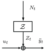
(a)

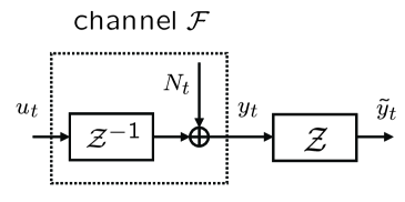
(b)

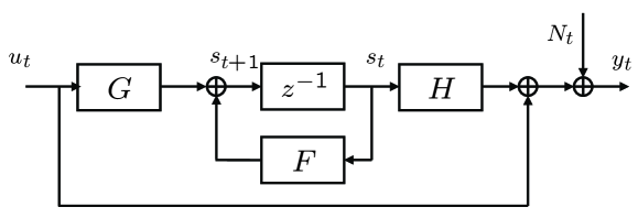
(c)

Figure 1: (a) A colored Gaussian noise channel without ISI. (b) The equivalent ISI channel with AWGN. (c) State-space realization of channel ${\mathcal{F}}$.

Note that there is no loss of generality in assuming that ${\mathcal{Z}}(z)$ is stable and minimum-phase (cf. Chapter 11, [26]), implying that the initial condition of ${\mathcal{Z}}(z)$ generates no effect on the steady-state. Thus we made the initial rest assumption since we mainly focus on the steady-state characterization.

II-B White Gaussian channel with ISI

The above colored Gaussian channel induces a new channel, namely a white Gaussian channel with ISI, under a further assumption that ${\mathcal{Z}}(\infty)\neq 0$ (i.e. ${\mathcal{Z}}$ is proper but non-strictly proper). More precisely, notice that from (2) and (3), we have

$$\tilde{y}^{T}={\mathcal{Z}}_{T}({\mathcal{Z}}_{T}^{-1}u^{T}+N^{T}),$$ (4)

which we identify as a stable and minimum-phase ISI channel with AWGN $\{N_{t}\}$, see Fig. 1 (b). Here ${\mathcal{Z}}^{-1}(z)$ is also at initial rest. For any fixed $u^{T}$ and $N^{T}$, (a) and (b) generate the same channel output $\tilde{y}^{T}$. Note that ${\mathcal{Z}}_{T}^{-1}$ is the matrix inverse of ${\mathcal{Z}}_{T}$, equal to the lower-triangular Toeplitz matrix of impulse response of ${\mathcal{Z}}^{-1}(z)$.

The initial rest assumption on ${\mathcal{Z}}^{-1}$ can be imposed in practice equivalently by, first driving the initial condition of the ISI channel to any desired value (known to the receiver) before a transmission, and then removing the response due to that initial condition at the receiver. Such an assumption is also used in [12, 11]. We further assume for simplicity that ${\mathcal{Z}}(\infty)=1$; for cases where $g:={\mathcal{Z}}(\infty)\neq 1$, we can normalize ${\mathcal{Z}}(z)$ by scaling it by $1/g$. Hence, ${\mathcal{Z}}_{T}$ is a lower triangular Toeplitz matrix with diagonal elements all equal to 1 (and thus is invertible).

We can then write the minimal state-space representation of ${\mathcal{Z}}^{-1}$ as $(F,G,H,1)$, where $F\in\mathbb{R}^{m}$ is stable, $(F,G)$ is controllable, $(F,H)$ is observable, and $m$ is the dimension or order of ${\mathcal{Z}}^{-1}$. Let us denote the channel from $u$ to $y$ in Fig. 1(b) as ${\mathcal{F}}$, where

$$y^{T}:={\mathcal{Z}}_{T}^{-1}u^{T}+N^{T}={\mathcal{Z}}_{T}^{-1}\tilde{y}^{T}.$$ (5)

The channel ${\mathcal{F}}$ is described in state-space as

$$\textnormal{channel }{\mathcal{F}}:\left\{\begin{array}[]{lll}s_{t+1}&=&Fs_{t}+Gu_{t}\\ y_{t}&=&Hs_{t}+u_{t}+N_{t},\end{array}\right.$$ (6)

where $s_{0}=0$; see Fig. 1 (c). Notice that channel ${\mathcal{F}}$ is not essentially different than the channel from $u$ to $\tilde{y}$, since $\{y^{t}\}$ and $\{\tilde{y}^{t}\}$ causally determine each other.

We concentrate on the case $m\geq 1$; the case that $m$ is 0 (i.e., ${\mathcal{F}}$ is an AWGN channel) was solved in [1, 2].

III Problem formulation in steady-state and the solution

Before formulating the steady-state communication problem, we distinguish among the three scenarios: Finite-horizon (i.e. finite coding length), infinite-horizon (i.e. infinite coding length), and steady state. Finite-horizon problems often have time-dependent (i.e. time-varying) and horizon-dependent solutions (similar to finite-horizon Kalman filtering). The horizon-dependence may be removed in the infinite-horizon scenario, and furthermore, the time-dependence may be removed in the steady-state scenario. If we find the (stationary, time-invariant) steady-state solution (which by [16] is also the infinite-horizon solution), we can truncate it and employ the truncation to the practical problem in finite-horizon provided that the horizon is large enough. This truncated solution would greatly simplify the implementation while having a performance sufficiently close to finite-horizon optimality.

III-A Problem formulation

For a Gaussian channel with feedback, the channel input may take the form

$$u_{t}=\gamma_{t}u^{t-1}+\eta_{t}y^{t-1}+\xi_{t}$$ (7)

for any $\gamma_{t}\in\mathbb{R}^{1\times t}$, $\eta_{t}\in\mathbb{R}^{1\times t}$, and zero-mean Gaussian random variable $\xi_{t}\in\mathbb{R}$ which is independent of $u^{t-1}$ and $y^{t-1}$ (cf. [11, 12]). Therefore, the channel inputs are allowed to depend on the channel outputs in a strictly causal manner. Our objective in this paper is to design encoder/decoder to achieve the asymptotic feedback capacity, given by

$$\begin{array}[]{lcl}C_{\infty}:=C_{\infty}({\mathcal{P}}):=&\displaystyle\sup_{\{u_{t}\}\textrm{ \small stationary,(\ref{u1})}}&\displaystyle\lim_{T\rightarrow\infty}\frac{1}{T+1}I(u^{T}\rightarrow y^{T})\\ &{}^{s.t.\>P_{\infty}:=\lim_{T\rightarrow\infty}\mathbf{E}u^{T}{}^{\prime}u^{T}/(T+1)\leq\mathcal{P}}&\end{array}$$ (8)

where ${\mathcal{P}}>0$ is the power budget and $I(u^{T}\rightarrow y^{T})$ is the directed information from $u^{T}$ to $y^{T}$ (cf. [11]). For more details about $C_{\infty}$, refer to [12, 16] and Section VII-A in this paper.

The problem of solving $C_{\infty}$ may be equivalently formulated as minimizing the average channel input power while keeping the information rate bounded from below, namely for ${\mathcal{R}}>0$,

$$\begin{array}[]{lcl}P_{\infty}({\mathcal{R}}):=&\displaystyle\inf_{\{u_{t}\}\textrm{ \small stationary,(\ref{u1})}}&\displaystyle\lim_{T\rightarrow\infty}\frac{1}{T+1}\mathbf{E}u^{T}{}^{\prime}u^{T}.\\ &{}^{s.t.\>\lim_{T\rightarrow\infty}I(u^{T}\rightarrow y^{T})/(T+1)\geq{\mathcal{R}}}&\end{array}$$ (9)

Therefore $P_{\infty}({\mathcal{R}})$ is the inverse function of $C_{\infty}({\mathcal{P}})$, i.e., $C_{\infty}(P_{\infty}({\mathcal{R}}))={\mathcal{R}}$.

Approach: Our approach to solve the steady-state communication problem is to investigate the finite-horizon problem first, and then let the horizon increase to infinity, which leads to a unified treatment of infinite-horizon and finite-horizon. Other approaches not pursued in this paper are also possible, such as applying the idea in [14] to the optimal signalling strategy in [12], though they generate results not as rich as the present approach does.

III-B The coding scheme

The rest of this section presents the solution to the above problem. In this subsection, we introduce an encoder/decoder structure and explain how to choose the parameters to ensure the optimality, and then describe the encoding/decoding process, that is, how we assign the message to be transmitted, and how we recover the message. In the next subsection, we present the coding theorem which states that our encoding/decoding structure with the chosen parameters achieves $C_{\infty}$. The proof of the theorem will be developed in Sections IV to VII.

The encoder/decoder structure

In state-space, the encoder and decoder are described as

$$\textnormal{Encoder:}\left\{\begin{array}[]{lll}x_{t+1}&=&Ax_{t}\\ r_{t}&=&Cx_{t}\\ u_{t}&=&r_{t}-\hat{r}_{t}\end{array}\right.$$ (10)

and

$$\textnormal{Decoder:}\left\{\begin{array}[]{lll}\hat{s}_{t+1}&=&F\hat{s}_{t}+L_{2}e_{t}\\ e_{t}&=&y_{t}-H\hat{s}_{t}\\ \hat{x}_{t+1}&=&A\hat{x}_{t}+L_{1}e_{t}\\ \hat{r}_{t}&=&C\hat{x}_{t}\\ \hat{x}_{0,t}&=&A^{-t-1}\hat{x}_{t+1},\end{array}\right.$$ (11)

where $\hat{s}_{0}=0$, $\hat{x}_{0}=0$, $A\in\mathbb{R}^{(n+1)\times(n+1)}$, $C\in\mathbb{R}^{1\times(n+1)}$, $L_{1}\in\mathbb{R}^{n+1}$, and $L_{2}\in\mathbb{R}^{m}$. We call $(n+1)$ the encoder dimension, $x_{t}$ the encoder state, and $\hat{x}_{0,t}$ the decoder estimate. See Fig. 2 for the block diagram. Observe that $-\hat{r}_{t}$ is the feedback from the decoder based on the channel output $y^{t-1}$, and thus $u_{t}$ depends on $y^{t-1}$ but not $y_{t}$. It further follows that $-\hat{r}^{t}={\mathcal{G}}^{*}_{t}y^{t}$ for some strictly lower triangular Toeplitz matrix ${\mathcal{G}}^{*}_{t}$. Here $A,C,u_{t}$, etc. depend on $n$, but we do not specify the dependence explicitly to simplify notations.

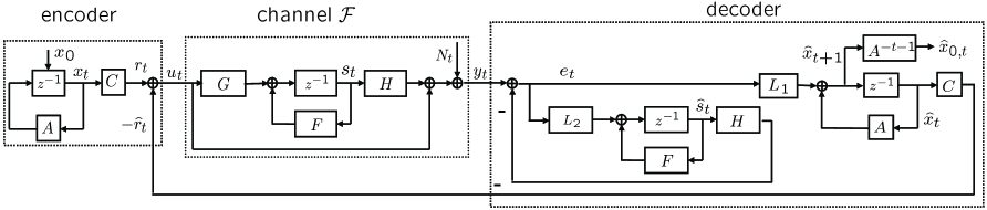
Figure 2: The encoder/decoder structure for ${\mathcal{F}}$.

Optimal choice of parameters

Fix a desired rate ${\mathcal{R}}$. Let $DI:=2^{\mathcal{R}}$ and $n:=m-1$ (recalling that $m$ is the channel dimension), and solve the optimization problem

$$\begin{array}[]{lcl}[\boldsymbol{a}_{f}^{opt},\Sigma^{opt}]:=&\displaystyle{\textnormal{arg}\inf_{\boldsymbol{a}_{f}\in\mathbb{R}^{n}}}&\mathbb{D}\Sigma\mathbb{D}^{\prime},\\ &{}^{s.t.\>\Sigma=\mathbb{A}\Sigma\mathbb{A}^{\prime}-\mathbb{A}\Sigma\mathbb{C}^{\prime}\mathbb{C}\Sigma\mathbb{A}^{\prime}/(\mathbb{C}\Sigma\mathbb{C}^{\prime}+1)}\end{array}\vspace{-10pt}$$ (12)

where

$$\mathbb{A}:=\left[\begin{array}[]{c|c}A&0\cr\hline\cr GC&F\end{array}\right],\mathbb{C}:=\left[\matrix{C&H}\right],\mathbb{D}:=\left[\matrix{C&0}\right],A:=\left[\begin{array}[]{c|c}0_{n\times 1}&I_{n}\cr\hline\cr\pm DI&\boldsymbol{a}_{f}\end{array}\right],C:=\left[\begin{array}[]{cc}1&0_{1\times n}\end{array}\right].$$ (13)

Note that we need to solve (12) twice (one for $+DI$ in $A$ and one for $-DI$ in $A$), and choose the optimal solution as the one with the smaller objective function value. Then we form the optimal $A^{opt}$ based on $\boldsymbol{a}_{f}^{opt}$, and let $(n^{*}+1)$ be the number of unstable eigenvalues in $A^{opt}$, where $n^{*}\geq 0$.

Now let $n:=n^{*}$, solve (12) again, and obtain a new $\boldsymbol{a}_{f}^{opt}$ and $\Sigma^{opt}$. Then form $A^{opt}$, let $A^{*}=A^{opt}$, $\Sigma^{*}=\Sigma^{opt}$, $C^{*}:=[1,0_{1\times n^{*}}]$, and form $\mathbb{A}^{*}$,$\mathbb{C}^{*}$, and $\mathbb{D}^{*}$. Let

$$L^{*}:=[L_{1}^{*}{}^{\prime},L_{2}^{*}{}^{\prime}]^{\prime}:=\frac{\mathbb{A}^{*}\Sigma^{*}\mathbb{C}^{*}{}^{\prime}}{\mathbb{C}^{*}\Sigma^{*}\mathbb{C}^{*}{}^{\prime}+1}.$$ (14)

As we will show, $(A^{*},C^{*})$ is observable, and $A^{*}$ has exactly $(n^{*}+1)$ unstable eigenvalues.

We assign the encoder/decoder parameters to the scheme built in Fig. 2 by letting

$$n:=n^{*},A:=A^{*},C:=C^{*},L_{1}:=L_{1}^{*},L_{2}:=L_{2}^{*}.$$ (15)

We then drive the initial condition $s_{0}$ of channel ${\mathcal{F}}$ to zero. Now we are ready to communicate at a rate ${\mathcal{R}}$ using power $P_{\infty}({\mathcal{R}})=\mathbb{D}^{*}\Sigma^{*}\mathbb{D}^{*}{}^{\prime}$.

Encoding/Decoding process

III-B1 Transmission of analog source

The designed communication system can transmit either an analog source or a digital message. In the former case, we assume that the encoder wishes to convey a Gaussian random vector through the channel and the decoder wishes to learn the random vector, which is a rate-distortion problem (or successive refinement problem, see e.g. [27, 13, 28]). The coding process is as follows. Assume that the to-be-conveyed message $W$ is distributed as ${\mathcal{N}}(0,I_{n^{*}+1})$ (noting that any non-degenerate $(n^{*}+1)$-variate Gaussian vector $W$ can be transformed into this form). Assume that the coding length is $(T+1)$. To encode, let $x_{0}:=W$. Then run the system till time epoch $T$, obtaining $\hat{x}_{0,t}$, $t=0,1,\cdots,T$. To decode, let $\hat{W}_{t}:=\hat{x}_{0,t}$ for $t=0,1,\cdots,T$.

The quantities of interest include the squared-error distortion, defined as

$$\mbox{MSE}(\hat{W}_{t}):=\mathbf{E}(W-\hat{W}_{t})(W-\hat{W}_{t})^{\prime}.$$ (16)

It will become clear that $\mbox{MSE}(\hat{W}_{t})$ can be pre-computed before the transmission, and thus the coding length can be determined a priori to ensure a desired distortion level.

III-B2 Transmission of digital message

To transmit digital messages over the communication system, let us first fix ${\epsilon}>0$ small enough and the coding length $(T+1)$ large enough. Let

$$\Sigma_{x}^{*}:=[I_{n^{*}+1},0]\Sigma^{*}[I_{n^{*}+1},0]^{\prime}.$$ (17)

Assume that the matrix $(A^{*}{}^{\prime})^{-T-1}\Sigma_{x}^{*}(A^{*})^{-T-1}$ has an eigenvalue decomposition as

$$(A^{*}{}^{\prime})^{-T-1}\Sigma_{x}^{*}(A^{*})^{-T-1}=E_{T}\Lambda_{T}E_{T}^{\prime},$$ (18)

where $E_{T}=[e^{(1)},\cdots,e^{(n^{*}+1)}]$ is an orthonormal matrix and $\Lambda_{T}$ is a positive diagonal matrix. Let $\sigma_{T,i}$ be the square root of the $(i,i)$th element of $\Lambda_{T}$. Let ${\mathcal{B}}\in\mathbb{R}^{n^{*}+1}$ be the unit hypercube spanned by columns of $E_{T}$, that is,

$${\mathcal{B}}=\left\{\left.\sum_{i=0}^{n^{*}}\alpha^{(i)}e^{(i)}\right|\alpha^{(i)}\in[-\frac{1}{2},\frac{1}{2}],i=0,\cdots,n^{*}\right\}.$$ (19)

Next we partition the $i$th side of ${\mathcal{B}}$ into $(\sigma_{T,i})^{-(1-\epsilon)}$ segments. This induces a partition of ${\mathcal{B}}$ into $M_{T}$ sub-hypercubes, where

$$\begin{array}[]{lll}M_{T}&=&\displaystyle\prod_{i=0}^{n^{*}}\left(\sigma_{T,i}\right)^{-(1-\epsilon)}\\ &=&\displaystyle\left[\det\left((A^{*}{}^{\prime})^{-T-1}\Sigma^{*}(A^{*})^{-T-1}\right)\right]^{-\frac{1-\epsilon}{2}}.\end{array}$$ (20)

We then map the sub-hypercube centers to a set of $M_{T}$ equally likely messages. The above procedure is known to both the transmitter and receiver a priori.

Suppose now we wish to transmit the message represented by the center $W$. To encode, let $x_{0}:=W$. Then run the system till time epoch $T$. To decode, we map $\hat{x}_{0,T}$ into the closest sub-hypercube center and obtain the decoded message $\hat{W}_{T}$. We declare an error if $\hat{W}_{T}\neq W$, and call a (an asymptotic) rate

$$R:=\lim_{T\rightarrow\infty}\frac{1}{T+1}\log M_{T}$$ (21)

achievable if the probability of error $PE_{T}$ vanishes as $T$ tends to infinity. We remark that this coding process is the one used in [14] for Gaussian channels with memory, which was an extension of the SK codes. In fact, the original SK coding scheme can be rewritten in a Kalman filter form, and hence it essentially implements the Kalman filtering algorithm. We also remark that, similar to the analog transmission case, the coding length $(T+1)$ can be pre-determined.

As we have seen, the encoder/decoder design and the encoding/decoding process can be done rather easily. The computation complexity for encoding/decoding grows as $O(T+1)$. Also interestingly, the encoder may be viewed as a control system, and the decoder may be viewed as an estimation system, as pointed out by Sanjoy Mitter and in [13, 29].

III-C Coding theorem

Theorem 1.

Construct the encoder/decoder shown in Fig. 2 using $n^{*}$, $A^{*}$, $C^{*}$, $L_{1}^{*}$, and $L_{2}^{*}$. Then under the power constraint $\mathbf{E}u^{2}\leq{\mathcal{P}}$,

i) The coding scheme transmits an analog source $W\sim{\mathcal{N}}(0,I_{n^{*}+1})$ from the encoder to the decoder at rate $C_{\infty}({\mathcal{P}})$, with MSE distortion $\mbox{MSE}(\hat{W}_{T})$ achieving the optimal asymptotic rate-distortion tradeoff given by

$$R=\lim_{T\rightarrow\infty}\frac{1}{2(T+1)}\log\frac{1}{\det\mbox{MSE}(\hat{W}_{T})}.$$ (22)

ii) The coding scheme can transmit digital message from the encoder to the decoder at a rate arbitrarily close to $C_{\infty}({\mathcal{P}})$, with $PE_{T}$ decays to zero doubly exponentially.

The proof of the theorem will be developed in the subsequent four sections. In Section IV, we consider a general coding structure in finite-horizon which may be viewed as a generalization of our optimal coding structure. We show that this general structure essentially contains a Kalman filter. The presence of the Kalman filter links the feedback communication problem to an estimation problem and a control problem, and hence we rewrite the information rate in terms of estimation theory quantities and control theory quantities; see Section V. Sections IV and V are focused on finite-horizon. In Section VI, we extend the horizon to infinity and characterize the steady-state behavior. Then in Section VII, we show that our optimal encoder/decoder design is actually the solution to the steady-state communication problem.

IV Necessity of Kalman filter for optimal coding

In this section, we consider a finite-horizon coding structure that includes our optimal design in Section III as a special case. This general structure is useful since: 1) searching over all possible parameters in the general structure achieves $C_{\infty}$, that is, there is no loss of generality or optimality to focus on this structure only; 2) we can show that to ensure power efficiency (to be explained), the general structure necessarily contains a Kalman filter. The general coding structure is in fact a variation of the CP structure (see Appendix B-D), and hence our Kalman filter characterization leads to a refinement of the CP structure.

IV-A A general coding structure

Fig. 3 illustrates the general coding structure, including the encoder and the feedback generator, a portion of the decoder. Below, we fix the time horizon to be $\{0,1,\cdots,T\}$ and describe the coding structure.

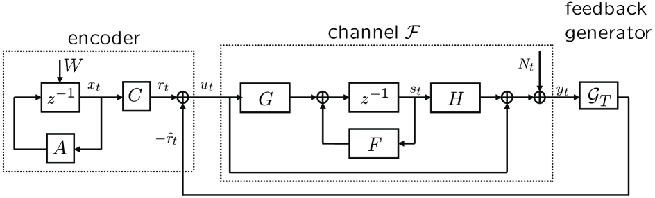
Figure 3: A general coding structure for channel ${\mathcal{F}}$.

Encoder: The encoder follows the dynamics (10). We assume that the encoder dimension $(n+1)$ satisfies $0\leq n\leq T$, $W\sim{\mathcal{N}}(0,I_{n+1})$, $A\in\mathbb{R}^{(n+1)\times(n+1)}$, $C\in\mathbb{R}^{1\times(n+1)}$, $(A,C)$ is observable, and none of the eigenvalues of $A$ are on the unit circle or at the locations of the eigenvalues of $F$. We then let

$$\begin{array}[]{lllll}\Gamma_{n}(A,C)&:=&\Gamma_{n}&:=&[C^{\prime},A^{\prime}C^{\prime},\cdots,A^{n}{}^{\prime}C^{\prime}]^{\prime}\\ \Gamma(A,C)&:=&\Gamma&:=&[C^{\prime},A^{\prime}C^{\prime},\cdots,A^{T}{}^{\prime}C^{\prime}]^{\prime}\\ K_{r}^{(T)}(A,C)&:=&K_{r}^{(T)}&:=&\mathbf{E}r^{T}r^{T}{}^{\prime}.\end{array}$$ (23)

Therefore, $\Gamma_{n}$ is the observability matrix for $(A,C)$ and is invertible, $\Gamma$ has rank $(n+1)$, $r^{T}=\Gamma W$, and $K_{r}^{(T)}=\Gamma\Gamma^{\prime}$.

Feedback generator: The feedback signal $-\hat{r}_{t}$ is generated through the feedback generator ${\mathcal{G}}_{T}$, i.e.

$$-\hat{r}^{T}={\mathcal{G}}_{T}y^{T}.$$ (24)

We assume that ${\mathcal{G}}_{T}\in\mathbb{R}^{(T+1)\times(T+1)}$ is a strictly lower triangular matrix. Clearly, the optimal encoder/decoder can be viewed as a special case of the general structure. Throughout the paper, the above assumptions on the encoder/decoder are always assumed unless otherwise specified. For future use purpose, we compute the channel output as

$$y^{T}=(I-{\mathcal{Z}}_{T}^{-1}{\mathcal{G}}_{T})^{-1}({\mathcal{Z}}_{T}^{-1}r^{T}+N^{T}).$$ (25)

Definition 1.

Consider the general coding structure shown in Fig. 3. Define

$$\begin{array}[]{lll}\displaystyle C_{T,n}:=C_{T,n}({\mathcal{P}})&:=&\displaystyle\sup_{A\in\mathbb{R}^{(n+1)\times(n+1)},C,{\mathcal{G}}_{T}}\frac{1}{T+1}I(W;y^{T})\\ &&{}^{s.t.\>\mathbf{E}u^{T}{}^{\prime}u^{T}/(T+1)\leq\mathcal{P}}\end{array}\vspace{-10pt}$$ (26)

and define its inverse function as $P_{T,n}({\mathcal{R}})$.

In other words, $C_{T,n}$ is the finite-horizon information capacity for a fixed transmitter dimension $n$. It holds that $C_{n,n}=C_{n}$ and hence $\lim_{n\rightarrow\infty}C_{n,n}=C_{\infty}$ (see Lemma 1 and Appendix C-B). Moreover, as we will show, $C_{\infty}$ can be achieved using this structure.

IV-B The presence of Kalman filter

We first compute the mutual information in the general coding structure.

Proposition 1.

Consider the general coding structure in Fig. 3. Fix any $0\leq n\leq T$, and fix any $A,C$, and ${\mathcal{G}}_{T}$. Then it holds that

$$\begin{array}[]{lll}I(W;y^{T})&=&I(r^{T};y^{T})\\ &=&I(u^{T}\rightarrow y^{T})\\ &=&\frac{1}{2}\log\det K_{y}^{(T)}\\ &=&\frac{1}{2}\log\det(I+{\mathcal{Z}}_{T}^{-1}K_{r}^{(T)}{\mathcal{Z}}_{T}^{-1^{\prime}})\\ &=&\frac{1}{2}\log\det(I+{\mathcal{Z}}_{T}^{-1}\Gamma\Gamma^{\prime}{\mathcal{Z}}_{T}^{-1^{\prime}}),\end{array}$$ (27)

which is independent of ${\mathcal{G}}_{T}$.

Proof:

$$\begin{array}[]{lll}I(W;y^{T})&=&h(y^{T})-h(y^{T}|W)\\ &=&h(y^{T})-h\left((I-{\mathcal{Z}}_{T}^{-1}{\mathcal{G}}_{T})^{-1}({\mathcal{Z}}_{T}^{-1}r^{T}+N^{T})|W\right)\\ &\stackrel{{\scriptstyle\textnormal{(a)}}}{{=}}&\frac{1}{2}\log\det(2\pi eK_{y}^{(T)})-h(N^{T})\\ &\stackrel{{\scriptstyle\textnormal{(b)}}}{{=}}&I(u^{T}\rightarrow y^{T})\\ &=&\frac{1}{2}\log\det K_{y}^{(T)}\\ &=&\frac{1}{2}\log\det(I+{\mathcal{Z}}_{T}^{-1}K_{r}^{(T)}{\mathcal{Z}}_{T}^{-1^{\prime}}),\end{array}$$ (28)

where (a) is due to $r^{T}=\Gamma W$, $\det(AB)=\det A\det B$, and $\det(I-{\mathcal{Z}}_{T}^{-1}{\mathcal{G}}_{T})^{-1}=1$; and (b) follows from [14]. ∎

Proposition 1 implies that $I(W;y^{T})$ is independent of the feedback generator ${\mathcal{G}}_{T}$, and dependent only on $K_{r}^{(T)}$ or equivalently on $(A,C)$. Thus, fixed $(A,C)$ implies fixed information rate, and hence the optimal feedback generator has to be chosen to minimize the average channel input power, which turns out to contain a Kalman filter. Note that the counterpart of this proposition in infinite-horizon was proven in [14]. Now we can define, for a fixed $(A,C)$, the information rate across the channel to be

$$R_{T}(A,C):=\frac{I(W;y^{T})}{T+1}.$$ (29)

The optimal feedback generator for a given $(A,C)$ is found in the next proposition.

Proposition 2.

Consider the general coding structure in Fig. 3. Fix any $0\leq n\leq T$. Then

i)

$$\begin{array}[]{llcllcl}P_{T,n}({\mathcal{R}})&=&\displaystyle\inf_{A,C,{\mathcal{G}}_{T}:={\mathcal{G}}_{T}^{*}(A,C)}&\displaystyle\frac{1}{T+1}\mathbf{E}u^{T}{}^{\prime}u^{T}\\ &&{}^{s.t.\>R_{T}(A,C)\geq{\mathcal{R}}}&\end{array}$$ (30)

where ${\mathcal{G}}_{T}^{*}(A,C)$ is the optimal feedback generator for a given $(A,C)$, defined as

$${\mathcal{G}}_{T}^{*}(A,C):=\arg\displaystyle\inf_{(A,C)\textnormal{ \small fixed},{\mathcal{G}}_{T}}\displaystyle\frac{1}{T+1}\mathbf{E}u^{T}{}^{\prime}u^{T}.$$ (31)

ii) The optimal feedback generator ${\mathcal{G}}_{T}^{*}(A,C)$ is given by

$${\mathcal{G}}_{T}^{*}(A,C)=-\widehat{\mathcal{G}}_{T}^{*}(A,C)(I-{\mathcal{Z}}_{T}^{-1}\widehat{\mathcal{G}}_{T}^{*}(A,C))^{-1},$$ (32)

where $\widehat{\mathcal{G}}_{T}^{*}(A,C)$ is the strictly causal MMSE estimator (Kalman filter) of $r^{T}$ given the noisy observation $\bar{y}^{T}:={\mathcal{Z}}_{T}^{-1}r^{T}+N^{T}$, i.e.,

$$\begin{array}[]{lll}\widehat{\mathcal{G}}_{T}^{*}(A,C)&:=&\displaystyle\arg\inf_{\widehat{\mathcal{G}}_{T}\in\mathbb{R}^{(T+1)\times(T+1)}}\displaystyle\frac{1}{T+1}\mathbf{E}(r^{T}-\widehat{\mathcal{G}}_{T}\bar{y}^{T})(r^{T}-\widehat{\mathcal{G}}_{T}\bar{y}^{T})^{\prime},\end{array}$$ (33)

where $\widehat{\mathcal{G}}_{T}$ is strictly lower triangular. See Fig. 4 (a) for the associated estimation problem, (b) for the Kalman filter $\widehat{\mathcal{G}}_{T}^{*}(A,C)$, and (c) for the optimal feedback generator ${\mathcal{G}}_{T}^{*}(A,C)$.

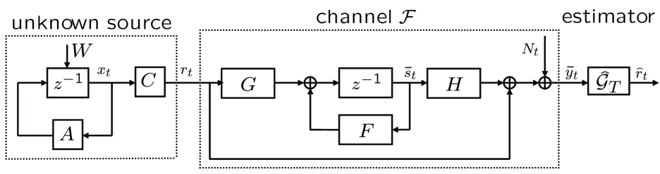
(a)

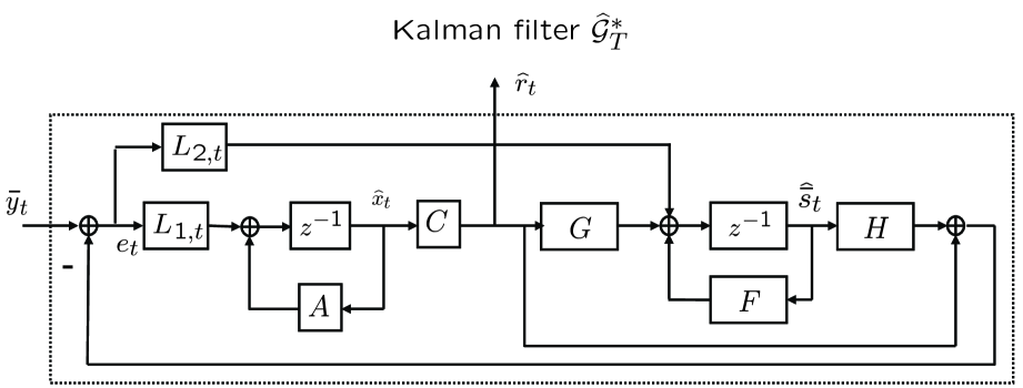
(b)

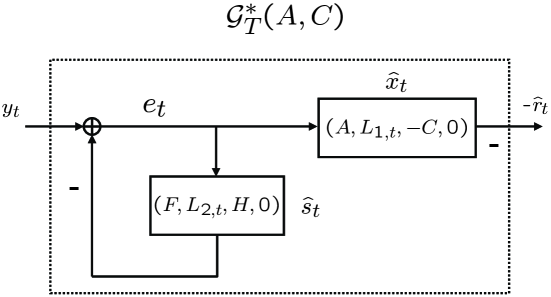
(c)

Figure 4: (a) An estimation problem over channel $\mathcal{F}$. (b) The Kalman filter $\widehat{\mathcal{G}}_{T}^{*}(A,C)$. (c) The Kalman filter based feedback generator ${\mathcal{G}}_{T}^{*}(A,C)$. Here $(A,L_{1,t},-C,0)$ with $\hat{x}_{t}$ denotes a state-space representation with $\hat{x}_{t}$ being its state at time $t$, and $\hat{x}_{0}$ being 0; see (41) and (44) for $L_{1,t}$ and $L_{2,t}$.

Remark 1.

Proposition 2 reveals that, the minimization of channel input power in a feedback communication problem is equivalent to the minimization of MSE in an estimation problem. This equivalence yields a complete characterization (in terms of the Kalman filter) of optimal feedback generator ${\mathcal{G}}_{T}^{*}(A,C)$ for a given $(A,C)$. Since our general coding structure is a variation of the CP structure, this proposition leads to the Kalman filter based characterization of the CP structure and hence is an improvement of the Cover-Pombra formulation; see Appendix B-D.

Remark 2.

Proposition 2 i) implies that we may reformulate the problem of $C_{T,n}$ (or $P_{T,n}$) as a two-step problem: In step 1, we fix $(A,C)$, i.e. fixing the rate, and minimize the input power by searching over ${\mathcal{G}}$; and in step 2, we search over all possible $(A,C)$ subject to the rate constraint. The role of the feedback generator ${\mathcal{G}}$ for any fixed $(A,C)$ is to minimize the input power. Then ii) solves the optimal feedback generator ${\mathcal{G}}_{T}^{*}(A,C)$ by considering the equivalent optimal estimation problem in Fig. 4 (a) whose solution is the Kalman filter. Notice that the Kalman filter can also give us the optimal estimate of the message $W$. Hence, the Kalman filter leads to both power efficiency and the best estimate of the message. The power efficiency is ensured by the one-step prediction operation of the Kalman filtering, and the optimal recovery of message is ensured by the smoothing operation of the Kalman filtering; therefore, we obtain the optimality of Kalman filtering in the information transmission sense. We finally note that the necessity of the Kalman filter is not surprising given the previous indications in [2, 5, 13, 11, 24], etc.

Proof:

i) Notice that for any fixed $(A,C)$, $R_{T}(A,C)$ is fixed. Then from the definition of $P_{T,n}({\mathcal{R}})$, we have

$$\begin{array}[]{llcll}P_{T,n}({\mathcal{R}})&=&\displaystyle\inf_{A,C,{\mathcal{G}}_{T}}&\displaystyle\frac{1}{T+1}\mathbf{E}u^{T}{}^{\prime}u^{T}\\ &&{}^{s.t.\>R_{T}(A,C)\geq{\mathcal{R}}}&\\ &=&\displaystyle\inf_{A,C}&\displaystyle\inf_{(A,C)\textnormal{ \small fixed},{\mathcal{G}}_{T}}&\displaystyle\frac{1}{T+1}\mathbf{E}u^{T}{}^{\prime}u^{T}\\ &&{}^{s.t.\>R_{T}(A,C)\geq{\mathcal{R}}}.&\end{array}$$ (34)

Then i) follows from the definition of ${\mathcal{G}}^{*}_{T}(A,C)$.

ii) Note that for the general coding structure, it holds that

$$u^{T}=r^{T}+(-\hat{r}^{T})=r^{T}+{\mathcal{G}}_{T}y^{T}.$$ (35)

Then, letting

$$\widehat{\mathcal{G}}_{T}:=-{\mathcal{G}}_{T}(I-{\mathcal{Z}}_{T}^{-1}{\mathcal{G}}_{T})^{-1}$$ (36)

and $\bar{y}^{T}:={\mathcal{Z}}_{T}^{-1}r^{T}+N^{T}$, we have ${\mathcal{G}}_{T}y^{T}=-\widehat{\mathcal{G}}_{T}\bar{y}^{T}$. Therefore,

$$\begin{array}[]{lll}{\mathcal{G}}_{T}^{*}(A,C)&=&\displaystyle\arg\inf_{{\mathcal{G}}_{T}}\displaystyle\frac{1}{T+1}\mathbf{E}(r^{T}+{\mathcal{G}}_{T}y^{T})(r^{T}+{\mathcal{G}}_{T}y^{T})^{\prime}\\ &=&\displaystyle\arg\inf_{\widehat{\mathcal{G}}_{T}}\displaystyle\frac{1}{T+1}\mathbf{E}(r^{T}-\widehat{\mathcal{G}}_{T}\bar{y}^{T})(r^{T}-\widehat{\mathcal{G}}_{T}\bar{y}^{T})^{\prime}.\end{array}$$ (37)

The last equality implies that the optimal solution $\widehat{\mathcal{G}}_{T}^{*}$ is the strictly causal MMSE estimator (with one-step prediction) of $r^{T}$ given $\bar{y}_{T}$; notice that $\widehat{\mathcal{G}}_{T}$ is strictly lower triangular. It is well known that such an estimator can be implemented recursively in state-space as a Kalman filter (cf. [30, 31]). Finally, from the relation between ${\mathcal{G}}_{T}$ and $\widehat{\mathcal{G}}_{T}$, we obtain (32). The state-space representation of ${\mathcal{G}}_{T}^{*}(A,C)$ needs only a straightforward computation, as shown in Appendix A. ∎

We remark that it is possible to derive a dynamic programming based solution ([11]) to compute $C_{T,n}$, and if we further employ the Markov property in [12] and the above Kalman filter based characterization, we would reach a solution with complexity $O(T)$ for computing $C_{T,n}$ and $C_{T}$. However, we do not pursue along this line in this paper since it is beyond the main scope of this paper.

V Feedback rate, CRB, and Bode integral

We have shown that in the general coding structure, to ensure power efficiency for a fixed $(A,C)$, we need to design a Kalman-filter based feedback generator. The Kalman filter immediately links the feedback communication problem to estimation and control problems. In this section, we present a unified representation for the general coding structure (with ${\mathcal{G}}$ being chosen as ${\mathcal{G}}^{*}(A,C)$), its estimation theory counterpart, and its control theory counterpart. Then we will establish connections among the information theory quantities, estimation theory quantities, and control theory quantities.

V-A Unified representation of feedback coding system, Kalman filter, and minimum-energy control

In this subsection, we will present the dynamics for the estimation problem and the general coding structure, then show that they are governed by one set of equations, which may also be viewed as a control system.

The estimation system

The estimation system in Fig. 4 consists of three parts: the unknown source $r^{T}$ to be estimated or tracked, the channel ${\mathcal{F}}$ (without output feedback), and the estimator which we choose as the Kalman filter $\widehat{\mathcal{G}}^{*}$; we assume that $(A,C)$ is fixed and known to the estimator. The system is described in state-space as

$$\textnormal{estimation system:}\left\{\begin{array}[]{ll}\begin{array}[]{lll}x_{t+1}&=&Ax_{t}\\ r_{t}&=&Cx_{t}\end{array}&\left.\begin{array}[]{l}\\ \end{array}\right\}\textnormal{unknown source}\\ \begin{array}[]{lll}\bar{s}_{t+1}&=&F\bar{s}_{t}+Gr_{t}\\ \bar{y}_{t}&=&H\bar{s}_{t}+r_{t}+N_{t}\end{array}&\left.\begin{array}[]{l}\\ \end{array}\right\}\textnormal{channel }{\mathcal{F}}\\ \begin{array}[]{lll}\hat{x}_{t+1}&=&A\hat{x}_{t}+L_{1,t}e_{t}\\ \hat{r}_{t}&=&C\hat{x}_{t}\\ \hat{\bar{s}}_{t+1}&=&F\hat{\bar{s}}_{t}+G\hat{r}_{t}+L_{2,t}e_{t}\\ e_{t}&=&\bar{y}_{t}-H\hat{\bar{s}}_{t}-\hat{r}_{t}\end{array}&\left.\begin{array}[]{l}\\ \\ \\ \\ \end{array}\right\}\textnormal{Kalman filter }\widehat{\mathcal{G}}^{*}(A,C)\end{array}\right.$$ (38)

with $x_{0}=W$, $\bar{s}_{0}=\hat{\bar{s}}_{0}=0$, and $\hat{x}_{0}=0$. Here $L_{1,t}\in\mathbb{R}^{n+1}$ and $L_{2,t}\in\mathbb{R}^{m}$ are the time-varying Kalman filter gains specified in (43).

The general coding structure with the optimal feedback generator

The optimal feedback generator for a given $(A,C)$ is solved in (32), see Fig. 4 (c) for its structure. We can then obtain the minimal state-space representation of ${\mathcal{G}}^{*}_{T}(A,C)$, and describe the general coding structure with ${\mathcal{G}}^{*}_{T}(A,C)$ as

$$\textnormal{general coding structure:}\left\{\begin{array}[]{ll}\begin{array}[]{lll}x_{t+1}&=&Ax_{t}\\ r_{t}&=&Cx_{t}\\ u_{t}&=&r_{t}-\hat{r}_{t}\end{array}&\left.\begin{array}[]{l}\\ \\ \end{array}\right\}\textnormal{encoder}\\ \begin{array}[]{lll}s_{t+1}&=&Fs_{t}+Gu_{t}\\ y_{t}&=&Hs_{t}+u_{t}+N_{t}\end{array}&\left.\begin{array}[]{l}\\ \end{array}\right\}\textnormal{channel }{\mathcal{F}}\\ \begin{array}[]{lll}\hat{s}_{t+1}&=&F\hat{s}_{t}+L_{2,t}e_{t}\\ e_{t}&=&y_{t}-H\hat{s}_{t}\\ \hat{x}_{t+1}&=&A\hat{x}_{t}+L_{1,t}e_{t}\\ -\hat{r}_{t}&=&-C\hat{x}_{t}\end{array}&\left.\begin{array}[]{l}\\ \\ \\ \end{array}\right\}\textnormal{optimal feedback generator }{\mathcal{G}}^{*}(A,C)\end{array}\right.$$ (39)

with $x_{0}=W$, $s_{0}=\hat{s}_{0}=0$, and $\hat{x}_{0}=0$. See Appendix A for the derivation of the minimal state-space representation of ${\mathcal{G}}^{*}_{T}(A,C)$. It can be easily shown that $r_{t}$, $\hat{r}_{t}$, $e_{t}$, $x_{t}$, and $\hat{x}_{t}$ in (38) and (39) are equal, respectively, and it holds that

$$s_{t}-\hat{s}_{t}=\bar{s}_{t}-\hat{\bar{s}}_{t}.$$ (40)

The unified representation

Define

$$\begin{array}[]{lll}\tilde{x}_{t}&:=&x_{t}-\hat{x}_{t}\\ \tilde{s}_{t}&:=&s_{t}-\hat{s}_{t}=\bar{s}_{t}-\hat{\bar{s}}_{t}\\ \mathbb{X}_{t}&:=&\left[\matrix{\tilde{x}_{t}\cr\tilde{s}_{t}}\right]\\ \mathbb{X}_{0}&:=&\left[\matrix{W\cr 0}\right]\\ \mathbb{A}&:=&\left[\begin{array}[]{c|c}A&0\\ \hline\cr GC&F\end{array}\right]\\ \mathbb{C}&:=&\left[\matrix{C&H}\right]\\ \mathbb{D}&:=&\left[\matrix{C&0}\right]\\ L_{t}&:=&\left[\matrix{L_{1,t}\cr L_{2,t}}\right].\end{array}$$ (41)

Note that $\mathbb{X}_{t}$ is the estimation error for $[x_{t}^{\prime},s_{t}^{\prime}]^{\prime}$. Substituting (41) to (38) and (39), we obtain that both systems become

$$\textnormal{control system:}\left\{\begin{array}[]{lll}\mathbb{X}_{t+1}&=&(\mathbb{A}-L_{t}\mathbb{C})\mathbb{X}_{t}-L_{t}N_{t}=\mathbb{A}\mathbb{X}_{t}-L_{t}e_{t}\\ e_{t}&=&\mathbb{C}\mathbb{X}_{t}+N_{t}\\ u_{t}&=&\mathbb{D}\mathbb{X}_{t};\end{array}\right.$$ (42)

see Fig. 5 for its block diagram. It is a control system where we want to minimize the power of $u$ by appropriately choosing $L_{t}$. This is a minimum energy control problem, which is useful for us to characterize the steady-state solution and it is equivalent to the Kalman filtering problem (see [32]).

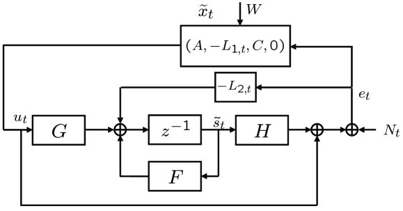
Figure 5: The block diagram for the minimum-energy control system. Here the block $(A,-L_{1,t},C,0)$ with $\tilde{x}_{t}$ denotes the state-space representation with $\tilde{x}_{t}$ and $W$ being its state at time $t$ and at time 0.

The signal $e_{t}$ in (42) is called the Kalman filter innovation or innovation , which plays a significant role in Kalman filtering. One fact is that $\{e_{t}\}$ is a white process, that is, its covariance matrix $K_{e}^{(T)}$ is a diagonal matrix. Another fact is that $e^{T}$ and $y^{T}$ determine each other causally, and we can easily verify that $h(e^{T})=h(y^{T})$ and $\det K_{y}^{(T)}=\det K_{e}^{(T)}$. We remark that (42) is the innovations representation of the Kalman filter (cf. [31]).

For each $t$, the optimal $L_{t}$ is determined as

$$L_{t}:=\left[\begin{array}[]{l}L_{1,t}\\ L_{2,t}\end{array}\right]:=\frac{\mathbb{A}\Sigma_{t}\mathbb{C}^{\prime}}{K_{e,t}},$$ (43)

where $\Sigma_{t}:=\mathbf{E}\mathbb{X}_{t}\mathbb{X}_{t}^{\prime}$, $K_{e,t}:=\mathbf{E}(e_{t})^{2}=\mathbb{C}\Sigma_{t}\mathbb{C}^{\prime}+1$, and the error covariance matrix $\Sigma_{t}$ satisfies the Riccati recursion

$$\Sigma_{t+1}=\mathbb{A}\Sigma_{t}\mathbb{A}^{\prime}-\frac{\mathbb{A}\Sigma_{t}\mathbb{C}^{\prime}\mathbb{C}\Sigma_{t}\mathbb{A}^{\prime}}{\mathbb{C}\Sigma_{t}\mathbb{C}^{\prime}+1}$$ (44)

with initial condition

$$\Sigma_{0}:=\left[\matrix{I_{n+1}&0\cr 0&0}\right],$$ (45)

This completes the description of the optimal feedback generator for a given $(A,C)$.

The meaning of a unified expression for three different systems (38), (39), and (42) is that the first two are actually two different non-minimal realizations of the third. The input-output mappings from $N^{T}$ to $e^{T}$ in the three systems are $T$-equivalent (see Appendix A-B). Thus we say that the three problems, the optimal estimation problem, the optimal feedback generator problem, and the minimum-energy control problem, are equivalent in the sense that, if any one of the problems is solved, then the other two are solved. Since the estimation problem and the control problem are well studied, the equivalence facilitates our study of the communication problem. Particularly, the formulation (42) yields alternative expressions for the mutual information and average channel input power in the feedback communication problem, as we see in the next subsection.

We further illustrate the relation of the estimation system and the communication system in Fig. 6: (b) is obtained from (a) by subtracting $\hat{r}_{t}$ from the channel input and adding ${\mathcal{Z}}_{T}^{-1}\hat{r}_{t}$ back to the channel output, which does not affect the input, state, and output of $\widehat{\mathcal{G}}_{T}^{*}$. It is clearly seen from the block diagram manipulations that the minimization of channel input power in feedback communication problem becomes the minimization of MSE in the estimation problem.

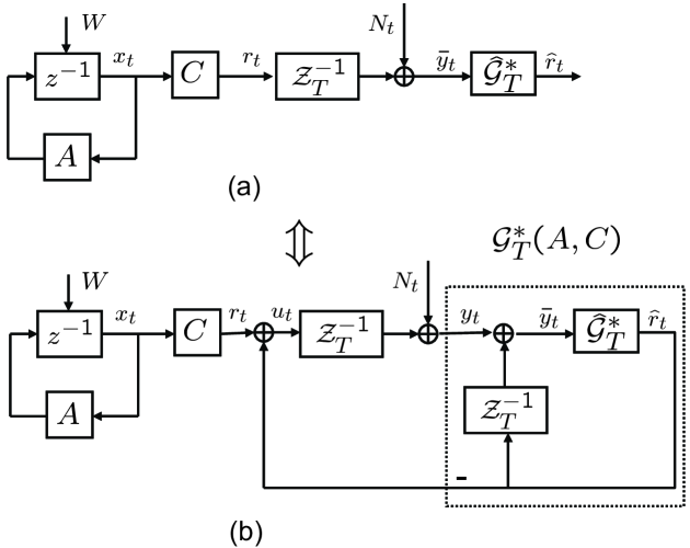
Figure 6: Relation between the estimation problem (a) and the communication problem (b).

V-B Mutual information in terms of Fisher information and CRB

Proposition 3.

For any fixed $0\leq n\leq T$ and $(A,C)$, it holds that

i)

$$\begin{array}[]{lll}I(W;y^{T})&=&\displaystyle\frac{1}{2}\log\det K_{e}^{(T)}=\frac{1}{2}\sum_{t=0}^{T}\log K_{e,t}\\ &=&\displaystyle\frac{1}{2}\sum_{t=0}^{T}\log(\mathbb{C}\Sigma_{t}\mathbb{C}^{\prime}+1)\\ &=&\displaystyle\frac{1}{2}\log\det\mbox{MMSE}_{W,T}^{-1}\\ &=&\displaystyle\frac{1}{2}\log\det{\mathcal{I}}_{W,T}\\ &=&\displaystyle\frac{1}{2}\log\det\textnormal{CRB}_{W,T}^{-1};\end{array}$$ (46)

ii)

$$\begin{array}[]{lll}P_{T,n}(A,C)&=&\displaystyle\frac{1}{T+1}\sum_{t=0}^{T}\mathbb{D}\Sigma_{t}\mathbb{D}^{\prime}\\ &=&\displaystyle\frac{1}{T+1}\textnormal{trace}(\mbox{CMMSE}_{r,T})\\ &=&\displaystyle\frac{1}{T+1}\sum_{t=0}^{T}CA^{t}\mbox{MMSE}_{W,t}A^{t}{}^{\prime}C^{\prime},\end{array}$$ (47)

where $\mbox{MMSE}_{W,T}$ is the minimum MSE of $W$, $\mbox{CMMSE}_{r,T}$ is the causal minimum MSE of $r^{T}$, ${\mathcal{I}}_{W,T}$ is the Bayesian Fisher information matrix of $W$ for the estimation system (38), and $\textnormal{CRB}_{W,T}$ is the Bayesian CRB of $W$ [33].

Remark 3.

This proposition connects the mutual information to the innovations process and to the Fisher information, (minimum) MSE, and CRB of the associated estimation problem. As a consequence, the finite-horizon feedback capacity $C_{T,n}$ is then linked to the smallest possible Bayesian CRB, i.e. the smallest possible estimation error covariance, and thus the fundamental limitation in information theory is linked to the fundamental limitation in estimation theory. It is also interesting to notice that the Fisher information, an estimation quantity, indeed has an information theoretic interpretation as its name suggests. Besides, the link between the mutual information and the MMSE provides a supplement to the fundamental relation discovered in [25]; the connections between our result and that in [25] is under current investigation.

Proof:

i) First we simply notice that $h(y^{T})=h(e^{T})$, and $K_{e,t}=\mathbb{C}\Sigma_{t}\mathbb{C}^{\prime}+1$. Next, to find MMSE of $W$, note that in Fig. 4 (a)

$$\bar{y}^{T}={\mathcal{Z}}_{T}^{-1}\Gamma W+N^{T}$$ (48)

and that $W\sim{\mathcal{N}}(0,I)$, $N^{T}\sim{\mathcal{N}}(0,I)$. Thus, by [30] we have

$$\mbox{MMSE}_{W,t}=(I+\Gamma^{\prime}{\mathcal{Z}}_{T}^{-1}{}^{\prime}{\mathcal{Z}}_{T}^{-1}\Gamma)^{-1},$$ (49)

yielding

$$\begin{array}[]{lll}\det\mbox{MMSE}_{W,t}&=&\det(I+{\mathcal{Z}}_{T}^{-1}\Gamma\Gamma^{\prime}{\mathcal{Z}}_{T}^{-1}{}^{\prime})^{-1}\\ &=&\det(I+{\mathcal{Z}}_{T}^{-1}K_{r}^{(T,n)}{\mathcal{Z}}_{T}^{-1}{}^{\prime})^{-1}.\end{array}$$ (50)

Besides, from Section 2.4 in [33] we can directly compute the FIM of $W$ to be $(I+\Gamma^{\prime}{\mathcal{Z}}_{T}^{-1}{}^{\prime}{\mathcal{Z}}_{T}^{-1}\Gamma)$. Then i) follows from Proposition 1 and (42).

ii) Since $u_{t}=\mathbb{D}\mathbb{X}_{t}=C\tilde{x}_{t}=r_{t}-\hat{r}_{t}$ and $\mathbf{E}\tilde{x}_{t}\tilde{x}_{t}^{\prime}=A^{t}\mbox{MMSE}_{W,t}A^{t}{}^{\prime}$, we have $\mathbf{E}(u_{t})^{2}=\mathbb{D}\Sigma_{t}\mathbb{D}^{\prime}=C\mathbf{E}\tilde{x}_{t}\tilde{x}_{t}^{\prime}C^{\prime}=\mathbf{E}(r_{t}-\hat{r}_{t})^{2}$, and then ii) follows. ∎

V-C Necessary condition for optimality

Before we turn to the infinite-horizon analysis, we show in this subsection that our general coding structure together with the optimal feedback generator satisfies a “necessary condition for optimality” discussed in [15]. The condition says that, the channel input $u_{t}$ needs to be orthogonal to the past channel outputs $y^{t-1}$. This is intuitive since to ensure fastest transmission, the transmitter should not transmit any information that the receiver has obtained, thus the transmitter wants to remove any correlation of $y^{t-1}$ in $u_{t}$ (to this aim, the transmitter has to access the channel outputs through feedback).

Proposition 4.

In system (39), for any $0\leq\tau<t$, it holds that $\mathbf{E}u_{t}y_{\tau}=0$.

Proof:

See Appendix B-E. ∎

VI Asymptotic behavior of the system

By far we have completed our analysis in finite-horizon. We have shown that the optimal design of encoder and decoder must contain a Kalman filter, and connected the feedback communication problem to an estimation problem and a control problem. Below, we consider the steady-state communication problem, by studying the limiting behavior ($T$ going to infinity) of the finite-horizon solution while fixing the encoder dimension to be $(n+1)$.

VI-A Convergence to steady-state

The time-varying Kalman filter in (42) converges to a steady-state, namely (42) is stabilized in closed-loop, $u_{t}$, $e_{t}$, and $y_{t}$ will converge to steady-state distributions, and $\Sigma_{t}$, $L_{t}$, ${\mathcal{G}}^{*}_{t}(A,C)$, $\widehat{\mathcal{G}}_{t}^{*}$, and $K_{e,t}$ will converge to their steady-state values. That is, asymptotically (42) becomes an LTI system

$$\textnormal{steady-state:}\left\{\begin{array}[]{lll}\mathbb{X}_{t+1}&=&(\mathbb{A}-L\mathbb{C})\mathbb{X}_{t}-LN_{t}=\mathbb{A}\mathbb{X}_{t}-Le_{t}\\ e_{t}&=&\mathbb{C}\mathbb{X}_{t}+N_{t}\\ u_{t}&=&\mathbb{D}\mathbb{X}_{t},\end{array}\right.$$ (51)

where

$$L:=\frac{\mathbb{A}\Sigma\mathbb{C}^{\prime}}{K_{e}},$$ (52)

$K_{e}=\mathbb{C}\Sigma\mathbb{C}^{\prime}+1$, and $\Sigma$ is the unique stabilizing solution to the Riccati equation

$$\Sigma=\mathbb{A}\Sigma\mathbb{A}^{\prime}-\frac{\mathbb{A}\Sigma\mathbb{C}^{\prime}\mathbb{C}\Sigma\mathbb{A}^{\prime}}{\mathbb{C}\Sigma\mathbb{C}^{\prime}+1}.$$ (53)

This LTI system is easy to analyze (e.g., it allows transfer function based study) and to implement. For instance, the minimum-energy control (cf. [32]) of an LTI system claims that the transfer function from $N$ to $e$ is an all-pass function in the form of

$${\mathcal{T}}_{Ne}(z)=\prod_{i=0}^{k}\frac{z-a_{i}}{z-a_{i}^{-1}}$$ (54)

where $a_{0},\cdots,a_{k}$ are the unstable eigenvalues of $A$ or $\mathbb{A}$ (noting that $F$ is stable). Note that this is consistent with the whiteness of innovations process $\{e_{t}\}$.

The existence of steady-state of the Kalman filter is proven in the following proposition. Notice that (42) is a singular Kalman filter since it has no process noise; the convergence of such a problem was established in [34].

Proposition 5.

Consider the Riccati recursion (44) and the system (42).

i) Starting from the initial condition given in (45), the Riccati recursion (44) generates a sequence $\{\Sigma_{t}\}$ that converges to $\Sigma_{\infty}$ with rank $(n+1)$, the unique stabilizing solution to the Riccati equation (53).

ii) The time-varying system (42) converges to the unique steady-state as given in (51).

Proof:

See Appendix C-A. ∎

VI-B Steady-state quantities

Now fix $(A,C)$ and let the horizon $T$ in the general coding structure go to infinity. Let $\mathcal{H}(e)$ be the entropy rate of $\{e_{t}\}$, $DI(A):=\prod_{i=0}^{k}|a_{i}|$ be the degree of instability of $A$, and $S(e^{j2\pi\theta})$ be the spectrum of the sensitivity function of system (51) (cf. [14]). Then the limiting result of Proposition 3 is summarized in the next proposition.

Proposition 6.

Consider the general coding structure in Fig. 3. For any $n\geq 0$ and $(A,C)$,

i) The asymptotic information rate is given by

$$\begin{array}[]{lll}R_{\infty,n}(A,C)&:=&\displaystyle\lim_{T\rightarrow\infty}\frac{1}{T+1}I(W;y^{T})\\ &=&\displaystyle\mathcal{H}(e)-\frac{1}{2}\log 2\pi e\\ &=&\displaystyle\log DI(A)\\ &=&\displaystyle\displaystyle\int_{-\frac{1}{2}}^{\frac{1}{2}}\log S(e^{j2\pi\theta})d\theta\\ &=&\displaystyle\frac{1}{2}\log(\mathbb{C}\Sigma\mathbb{C}^{\prime}+1)\\ &=&\displaystyle\lim_{T\rightarrow\infty}\frac{\log\det{\mathcal{I}}_{W,T}}{2(T+1)}\\ &=&\displaystyle-\lim_{T\rightarrow\infty}\frac{\log\det\mbox{MSE}_{W,T}}{2(T+1)}\\ &=&\displaystyle-\lim_{T\rightarrow\infty}\frac{\log\det\mbox{CRB}_{W,T}}{2(T+1)}.\end{array}$$ (55)

ii) The average channel input power is given by

$$\begin{array}[]{lll}P_{\infty,n}(A,C)&:=&\displaystyle\lim_{T\rightarrow\infty}\frac{1}{T+1}\mathbf{E}u_{T}u_{T}^{\prime}\\ &=&\displaystyle\mathbb{D}\Sigma\mathbb{D}^{\prime}.\end{array}$$ (56)

Remark 4.

Proposition 6 links the asymptotic information rate to the entropy rate of the innovations process, to the degree of instability and Bode sensitivity integral ([14]), to the asymptotic increasing rate of the Fisher information, and to the asymptotic decay rate of MSE and of CRB. Recall that the Bode sensitivity integral is the fundamental limitation of the disturbance rejection (control) problem, and the asymptotic decay rate of CRB is the fundamental limitation of the recursive estimation problem. Hence, the fundamental limitations in feedback communication, control, and estimation coincide.

Remark 5.

Proposition 6 implies that the presence of stable eigenvalues in $A$ does not affect the rate (see also [14]). Stable eigenvalues do not affect $P_{\infty,n}(A,C)$, either, since the initial condition response associated with the stable eigenvalues can be tracked with zero power (i.e. zero MSE). So, we can achieve $C_{\infty,n}$ by a sequence of purely unstable $(A,C)$, and hence the communication problem is related to the tracking of purely unstable source over a communication channel ([13, 14]).

Proof:

Proposition 6 leads to that, the limits of the results in Proposition 3 are well defined. Then

$$\begin{array}[]{lll}R_{\infty,n}(A,C)&=&\displaystyle\lim_{T\rightarrow\infty}\frac{1}{2(T+1)}\sum_{t=0}^{T}\log K_{e,t}\\ &=&\displaystyle\lim_{T\rightarrow\infty}\frac{1}{2}\log K_{e,t}\\ &=&\displaystyle\mathcal{H}(e)-\frac{1}{2}\log 2\pi e,\end{array}$$ (57)

where the second equality is due to the Cesaro mean (i.e., if $a_{k}$ converges to $a$, then the average of the first $k$ terms converges to $a$ as $k$ goes to infinity), and the last equality follows from the definition of entropy rate of a Gaussian process (cf. [35]).

Now by (54), $\{e_{t}\}$ has a flat power spectrum with magnitude $DI(A)^{2}$. Then $R_{\infty,n}(A,C)=\log DI(A)$. The Bode integral of sensitivity follows from [14]. The other equalities are the direct applications of the Cesaro mean to the results in Proposition 3. ∎

VII Achievability of $C_{\infty}$

In this section, we will prove that $C_{\infty,m-1}=C_{\infty}$, leading to the optimality of our encoder/decoder design in Section III in the mutual information sense, and then show that our design achieves $C_{\infty}$ in the operational sense.

VII-A The optimal Gauss-Markov signalling strategy and a simplification

[12] proved that for each input in the form of (7), there exists a Gauss-Markov (GM) input that yields the same directed information and same input power. The GM input takes the form

$$u_{t}=d_{t}^{\prime}\tilde{s}_{s,t}+{\mathcal{E}}_{t},$$ (58)

where $d_{t}\in\mathbb{R}^{m}$ is a time-varying gain; $\{{\mathcal{E}}_{t}\}$ is a zero-mean white Gaussian process and ${\mathcal{E}}_{t}$ is independent on $N^{t-1}$, $u^{t-1}$, and $y^{t-1}$; and $\tilde{s}_{s,t}$ is generated by a Kalman filter (noting that this Kalman filter is different from the Kalman filter obtained in this paper)

$$\left\{\begin{array}[]{lll}\tilde{s}_{s,t}&:=&s_{t}-\hat{s}_{s,t}\\ \hat{s}_{s,t+1}&=&F\hat{s}_{s,t}+L_{s,t}e_{t}\\ e_{t}&=&y_{t}-H\hat{s}_{s,t},\end{array}\right.$$ (59)

where $\hat{s}_{s,0}=0$,

$$L_{s,t}:=\frac{Q_{t}\Sigma_{s,t}(H+d_{t}^{\prime})^{\prime}+K_{{\mathcal{E}}}^{(t)}G}{1+K_{{\mathcal{E}}}^{(t)}+(H+d_{t}^{\prime})\Sigma_{s,t}(H+d_{t}^{\prime})^{\prime}},$$ (60)

$Q_{t}:=F+Gd_{t}^{\prime}$, and $\Sigma_{s,t}:=\mathbf{E}\tilde{s}_{s,t}\tilde{s}_{s,t}^{\prime}$ is the estimation error covariance of $s_{t}$, satisfying the Riccati recursion

$$\Sigma_{s,t+1}=Q_{t}\Sigma_{s,t}Q_{t}^{\prime}+K_{\mathcal{E}}^{(t)}GG^{\prime}-\frac{(Q_{t}\Sigma_{s,t}(H+d_{t}^{\prime})^{\prime}+K_{\mathcal{E}}^{(t)}G)(Q_{t}\Sigma_{s,t}(H+d_{t}^{\prime})^{\prime}+K_{\mathcal{E}}^{(t)}G)^{\prime}}{1+K_{{\mathcal{E}}}^{(t)}+(H+d_{t}^{\prime})\Sigma_{s,t}(H+d_{t}^{\prime})^{\prime}}.$$ (61)

If one lets $d_{t}=d$ and $K_{{\mathcal{E}}}^{(t)}=K_{{\mathcal{E}}}$ for all $t$, that is, the input $\{u_{t}\}$ is a stationary process, then the search over all possible $d$ and $K_{{\mathcal{E}}}$ solves $C_{\infty}$, that is,

$$\begin{array}[]{ccl}C_{\infty}({\mathcal{P}})=&\displaystyle{\max_{d\in\mathbb{R}^{m},K_{\mathcal{E}}\in\mathbb{R}}}&\displaystyle\frac{1}{2}\log(1+K_{\mathcal{E}}+(H+d^{\prime})\Sigma_{s}(H+d^{\prime})^{\prime})\par\end{array}$$ (62)

subject to Riccati equation constraint and power constraint

$$\begin{array}[]{lll}\Sigma_{s}&=&Q\Sigma_{s}Q^{\prime}+K_{\mathcal{E}}GG^{\prime}-\frac{(Q\Sigma_{s}(H+d^{\prime})^{\prime}+K_{\mathcal{E}}G)(Q\Sigma_{s}(H+d^{\prime})^{\prime}+K_{\mathcal{E}}G)^{\prime}}{1+K_{\mathcal{E}}+(H+d^{\prime})\Sigma_{s}(H+d^{\prime})^{\prime}}\\ {\mathcal{P}}&=&d^{\prime}\Sigma_{s}d+K_{\mathcal{E}}.\end{array}$$ (63)

We remark that [12] was focused more on the structure of the optimal input distribution and capacity computation, instead of designing a coding scheme; how to encode/decode a message (rather than using a random coding argument) is not clear from [12].

Now we prove that $K_{{\mathcal{E}}}=0$, namely $\{{\mathcal{E}}_{t}\}$ vanishes in steady-state. This leads to a further simplification of the results in [12].

Proposition 7.

For the GM input (58) to achieve $C_{\infty}$, it must hold that $K_{\mathcal{E}}=0$.

Proof:

See Appendix D. ∎

The vanishing of $\{{\mathcal{E}}_{t}\}$ in steady-state helps us to show that, our general coding structure shown in Fig. 3 can achieve $C_{\infty}$, and the encoder dimension needs not be higher than the channel dimension, namely to achieve $C_{\infty}$ we need $A$ to have at most $m$ unstable eigenvalues, as we will see in the next subsection.

VII-B Generality of the general coding structure; finite dimensionality of the optimal solution

In this subsection, we show that the general coding structure is sufficient to achieve mutual information $C_{\infty}$. In other words, if we search over all admissible parameters $A,C,{\mathcal{G}}_{T}$ in the general coding structure, allowing $T$ to increase to infinity and $n$ to increase to $(m-1)$, then we can obtain $C_{\infty}$. Thus, there is no loss of generality and optimality to consider only the general coding structure with encoder dimension no greater than $m$.

Definition 2.

Consider the general coding structure in Fig. 3. Let

$$C_{\infty,n}:=C_{\infty,n}({\mathcal{P}}):=\displaystyle\sup_{A\in\mathbb{R}^{(n+1)\times(n+1)},C,{\mathcal{G}}_{\infty}}\lim_{T\rightarrow\infty}\frac{1}{T+1}I(W;y^{T})$$ (64)

subject to

$$P_{\infty,n}:=\lim_{T\rightarrow\infty}\frac{1}{T+1}\mathbf{E}u^{T}{}^{\prime}u^{T}\leq\mathcal{P}.$$ (65)

In other words, $C_{\infty,n}$ is the infinite-horizon information capacity for a fixed transmitter dimension. Note that $C_{\infty,n}$ exists and is finite. To see this, note Proposition 6, $C_{\infty,n}\leq C_{\infty}<\infty$, and the fact that

$$C_{\infty,n}({\mathcal{P}})=\sup_{A\in\mathbb{R}^{(n+1)\times(n+1)},C,{\mathcal{G}}^{*}(A,C),(\ref{constr:cinfn})}R_{\infty,n}(A,C).$$ (66)

The function $C_{\infty,n}({\mathcal{P}})$ also induce $P_{\infty,n}({\mathcal{R}})$, the “capacity” in terms of minimum input power subject to an information rate constraint.

Proposition 8.

Consider the general coding structure in Fig. 3.

i) $C_{\infty,n}$ is increasing in $n$;

ii) For channel ${\mathcal{F}}$ with order $m\geq 1$, $C_{\infty,n}=C_{\infty}$ for $n\geq m-1$.

Proof:

See Appendix E-A. ∎

This proposition suggests that, to achieve $C_{\infty}$, we may first fix the transmitter dimension as $(n+1)$ and let the dynamical system run to time infinity, obtaining $C_{\infty,n}$, and then increase $n$ to $(m-1)$. The finite dimensionality of the optimal solution is important since it guarantees that we can achieve $C_{\infty}$ without solving an infinite-dimensional optimization problem.

VII-C Achieving $C_{\infty}$

In this subsection, we prove that our coding scheme achieves $C_{\infty}$ in the information sense as well as in the operational sense.

Proposition 9.

For the coding scheme described in Theorem 1, $R_{\infty,n^{*}}(A^{*},C^{*})=C_{\infty}({\mathcal{P}})$ and
$P_{\infty,n^{*}}$ $(A^{*},C^{*})={\mathcal{P}}$.

Proof:

See Appendix E-B. ∎

Proposition 10.

The system constructed in Theorem 1 transmits the analog source $W\sim{\mathcal{N}}(0,I)$ at a rate $C_{\infty}({\mathcal{P}})$, with MSE distortion $D(C_{\infty}({\mathcal{P}}))$, where $D(\cdot)$ is the distortion-rate function.

Proof:

See Appendix E-C. ∎

Proposition 11.

The system constructed in Theorem 1 transmits a digital message $W$ from the transmitter to the receiver at a rate arbitrarily close to $C_{\infty}({\mathcal{P}})$ with $PE_{T}$ decays doubly exponentially.

Proof:

See Appendix E-D. ∎

Note that, the coding length needed for a pre-specified performance level can be pre-determined since $\Sigma_{x,T}^{*}$ can be solved off-line. Besides, because the probability of error decays doubly exponentially, it leads to much shorter coding length than forward transmission.

VIII Numerical example

Here we repeat the numerical example studied in [12]. Consider a third-order channel (i.e. $m=3$) with

$${\mathcal{Z}}^{-1}:=\frac{1+0.5z^{-1}-0.4z^{-2}}{1+0.6z^{-2}-0.4z^{-3}}.$$ (67)

In state-space, ${\mathcal{Z}}^{-1}$ is described as $(F,G,H,1)$ where

$$\begin{array}[]{llllll}F&=&\left[\matrix{0&-0.6&0.4\cr 1&0&0\cr 0&1&0}\right]&\;G&=&\left[\matrix{1\cr 0\cr 0}\right]\\ H&=&\left[\matrix{0.5&-1&0.4}\right].&\end{array}$$ (68)

Assume the desired communication rate ${\mathcal{R}}$ is 1 bit per channel use. We first solve (12) with $n=m-1=2$, and find out $n^{*}=1$. That is, $C_{\infty}$ is attained when $A$ has two unstable eigenvalues. Then we solve (12) again with $n^{*}=1$, and obtain

$$\begin{array}[]{llllll}A^{*}&=&\left[\matrix{0&1\cr-2&-0.887}\right]\\ L^{*}&=&[\matrix{-0.506&-0.225&0.573&0.092&-0.327}]^{\prime}.&\end{array}$$ (69)

This yields the optimal power $P_{\infty}=0.743$ (or -1.290 dB). Similar computation generates Figure 7, the curve of $C_{\infty}$ against SNR or equivalently ${\mathcal{P}}$. This curve is identical to that in [12].

\psfragscanon\psfrag{alpha}{ $C_{\infty}$}\includegraphics{fbff1}

Figure 7: The asymptotic feedback capacity $C_{\infty}$ and feedforward capacity for channel ${\mathcal{F}}$ with ${\mathcal{Z}}^{-1}=(1+0.5z^{-1}-0.4z^{-2})/(1+0.6z^{-2}-0.4z^{-3})$.

We then use the obtained $A^{*}$, $C^{*}$, and $L^{*}$ to construct the optimal communication scheme. However, we observe that the optimal communication scheme shown in Fig. 2 generates unbounded signals $\{r_{t}\}$ and $\{\hat{r}_{t}\}$ due to the instability of $A$. This is not desirable for the simulation purpose, though the scheme in the form of Fig. 2 is convenient for the analysis purpose. Here, we propose a modification of the scheme, see Fig. 8. It is easily verify that the system in Fig. 8 is $T$-equivalent to that in Fig. 2. As we indicate in Fig. 8, the loop including the encoder, the channel, and the feedback link is indeed the control setup, which is stabilized and hence any signal inside is bounded. Note that the encoder now involves $\tilde{x}_{-1}$; we set $\tilde{x}_{-1}:=A^{-1}W$, leading to $\tilde{x}_{0}=W$, the desired value for $\tilde{x}_{0}$.

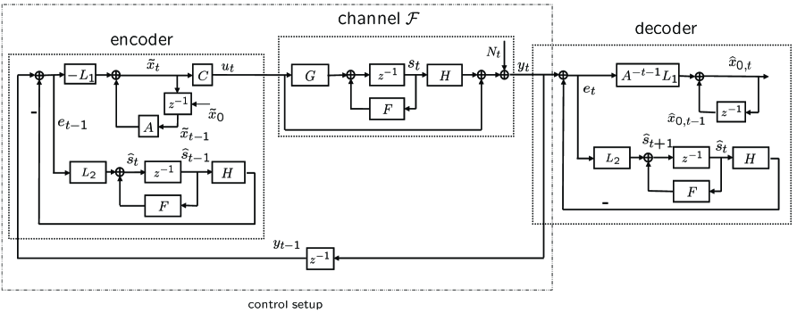
Figure 8: The modified feedback communication scheme.

We report the simulation results using the modified communication scheme with the optimal parameters given in (69). Fig. 9 (a) shows the convergence of $\hat{x}_{0,t}$ to $x_{0}$, in which $x_{0}:=[-0.2,-0.7]^{\prime}$. Fig. 9 (a) also shows the time average of the channel input power, which converges to the optimal power $P_{\infty}=0.743$. To compute the probability of error, we let ${\epsilon}=0.2$, i.e., the signalling rate is equal to $0.8C_{\infty}$. We demonstrate that this signalling rate is achieved by showing that the simulated probability of error decays to zero, see Fig. 9 (b). Fig. 9 (b) also plots the theoretic probability of error computed from (137), which is almost identical to the simulated curve. In addition, we see that the probability of error decays rather fast within 28 channel uses. The fast decay implies that the proposed scheme allows shorter coding length and shorter coding delay; here coding delay measures the time steps that one has to wait for the message to be decoded at the receiver with small enough error probability.

\psfrag{x0h1}{ \Large$\hat{x}_{0,t}^{(1)}$}\psfrag{x0h2}{\Large$\hat{x}_{0,t}^{(2)}$}\psfragscanon\psfrag{t}{ \LARGE{time} \LARGE$t$}\includegraphics{mod_one}

(a)

\psfrag{x0h1}{ \Large$\hat{x}_{0,t}^{(1)}$}\psfrag{x0h2}{\Large$\hat{x}_{0,t}^{(2)}$}\psfragscanon\psfrag{t}{ \LARGE{time} \LARGE$t$}\psfragscanon\psfrag{t}{\huge{number of channel uses} \LARGE$(T+1)$}\includegraphics{mtrial1_3_paper}

(b)

Figure 9: (a) Convergence of $\hat{x}_{0,t}$ to $x_{0}$, and convergence of the average channel input power. (b) Simulated probability of error and theoretic probability of error.

IX Conclusions and future work

We presented a coding scheme to achieve the asymptotic capacity $C_{\infty}$ for a Gaussian channel with feedback. The scheme is essentially the Kalman filter algorithm, and its construction involves only a finite dimensional optimization problem. We established connections of feedback communication to estimation and control. We have seen that concepts in estimation theory and control theory, such as MMSE, CRB, minimum-energy control, etc., are useful in studying a feedback communication system. We also verified the results by simulations.

Our ongoing research includes convexifying the optimization problem (12) to reduce the computation complexity, and finding a more feasible scheme to fight against feedback noise while keeping the feedback signal bounded. In future, we will further explore the connections among information, estimation, and control in more general setups (such as MIMO channels with feedback).

Appendix A Systems representations and equivalence

The concept of system representations and the equivalence between different representations are extensively used in this paper. In this subsection, we briefly introduce system representations and the equivalence. For more thorough treatment, see e.g. [37, 38, 39].

A-A Systems representations

Any discrete-time linear system can be represented as a linear mapping (or a linear operator) from its input space to output space; for example, we can describe a single-input single-output (SISO) linear system as

$$y^{t}={\mathcal{M}}_{t}u^{t}$$ (70)

for any $t$, where ${\mathcal{M}}_{t}\in\mathbb{R}^{(t+1)\times(t+1)}$ is the matrix representation of the linear operator, $u^{t}\in\mathbb{R}^{t+1}$ is the stacked input vector consisting of inputs from time 0 to time $t$, and $y^{t}\in\mathbb{R}^{t+1}$ is the stacked output vector consisting of outputs from time 0 to time $t$. For a (strictly) causal SISO LTI system, ${\mathcal{M}}_{t}$ is a (strictly) lower-triangular Toeplitz matrix formed by the coefficients of the impulse response. Such a system may also be described as the (reduced) transfer function, whose inverse $z$-transform is the impulse response; by a (reduced) transfer function we mean that its zeros are not at the same location of any pole.

A causal SISO LTI system can be realized in state-space as

$$\left\{\begin{array}[]{lll}x_{t+1}&=&Ax_{t}+Bu_{t}\\ y_{t}&=&Cx_{t}+Du_{t},\end{array}\right.$$ (71)

where $x_{t}\in\mathbb{R}^{l}$ is the state, $u_{t}\in\mathbb{R}$ is the input, and $y_{t}\in\mathbb{R}$ is the output. We call $l$ the dimension or the order of the realization. The state-space representation (71) may be denoted as $(A,B,C,D)$. Note that in the study of input-output relations, it is sometimes convenient to assume that the system is relaxed or at initial rest (i.e. zero input leads to zero output), whereas in the study of state-space, we generally allow $x_{0}\neq 0$, which is not at initial rest. For multi-input multi-output (MIMO) systems, linear time-varying systems, etc., see [38, 39].

The state-space representation of an causal FDLTI system ${\mathcal{M}}(z)$ is not unique. We call a realization $(A,B,C,D)$ minimal if $(A,B)$ is controllable and $(A,C)$ is observable. All minimal realizations of ${\mathcal{M}}(z)$ have the same dimension, which is the minimum dimension of all possible realizations. All other realizations are called non-minimal.

An example

We demonstrate here how we can derive a minimal realization of a system. Consider ${\mathcal{G}}_{T}^{*}(A,C)$ in (32) in Section IV, which is given by

$${\mathcal{G}}_{T}^{*}(A,C)=-\widehat{\mathcal{G}}_{T}^{*}(I-{\mathcal{Z}}_{T}^{-1}\widehat{\mathcal{G}}_{T}^{*})^{-1},$$ (72)

where the state-space representations for $\widehat{\mathcal{G}}_{T}^{*}(A,C)$ and ${\mathcal{Z}}_{T}^{-1}$ are illustrated in Fig. 6 (b) and Fig. 1 (c). Since (72) suggests a feedback connection of $\widehat{\mathcal{G}}^{*}$ and ${\mathcal{Z}}^{-1}$ as shown in Fig. 10, we can write the state-space for ${\mathcal{G}}^{*}$ as

$$\left\{\begin{array}[]{lll}\hat{x}_{t+1}&=&A\hat{x}_{t}+L_{1,t}e_{t}\\ \hat{r}_{t}&=&C\hat{x}_{t}\\ \hat{\bar{s}}_{t+1}&=&F\hat{\bar{s}}_{t}+G\hat{r}_{t}+L_{2,t}e_{t}\\ e_{t}&=&\bar{y}_{t}-H\hat{\bar{s}}_{t}-\hat{r}_{t}\\ s_{a,t+1}&=&Fs_{a,t}+G\hat{r}_{t}\\ \bar{y}_{t}&=&y_{t}+Hs_{a,t}+\hat{r}_{t}.\end{array}\right.$$ (73)

Then let $\hat{s}_{t}:=\hat{\bar{s}}_{t}-s_{a,t}$, and we have

$$\left\{\begin{array}[]{lll}\hat{x}_{t+1}&=&A\hat{x}_{t}+L_{1,t}e_{t}\\ \hat{r}_{t}&=&C\hat{x}_{t}\\ \hat{s}_{t+1}&=&F\hat{s}_{t}+L_{2,t}e_{t}\\ e_{t}&=&y_{t}-H\hat{s}_{t}.\end{array}\right.$$ (74)

It is straightforward to check that this dynamics is controllable and observable, and therefore it is a minimum realization of ${\mathcal{G}}^{*}$.

Figure 10: ${\mathcal{G}}^{*}$ is a feedback connection of $\widehat{\mathcal{G}}^{*}$ and ${\mathcal{Z}}^{-1}$.

A-B Equivalence between representations

Definition 3.

i) Two FDLTI systems represented in state-space are said to be equivalent if they admit a common transfer function (or a common transfer function matrix) and they are both stabilizable and detectable.

ii) Fix $0\leq T<\infty$. Two linear mappings ${\mathcal{M}}_{i,T}:\>\mathbb{R}^{q(T+1)}\rightarrow\mathbb{R}^{p(T+1)}$, $i=1,2$, both at initial rest, are said to be $T$-equivalent if for any $u^{T}\in\mathbb{R}^{q(T+1)}$, it holds that

$${\mathcal{M}}_{1,T}(u^{T})={\mathcal{M}}_{2,T}(u^{T}).$$ (75)

We note that i) is defined for FDLTI systems, whereas ii) is for general linear systems. i) implies that, the realizations of a transfer function are not necessarily equivalent. However, if we focus on all realizations that do not “hide” any unstable modes, namely all the unstable modes are either controllable from the input or observable from the output, they are equivalent; the converse is also true. ii) concerns about the finite-horizon input-output relations only. Since the states are not specified in ii), it is not readily extended to infinite horizon: Any unstable modes “hidden” from the input and output will grow unboundedly regardless of input and output, which is unwanted.

Examples

As we mentioned in Section II-B, for any $u^{T}$ and $N^{T}$, Fig. 1 (a) and (b) generate the same channel output $\tilde{y}^{T}$. That is, the mappings from $(u^{T},N^{T})$ to $\tilde{y}^{T}$ for the two channels are identical, and both are given by

$$\tilde{y}^{T}={\mathcal{Z}}_{T}({\mathcal{Z}}_{T}^{-1}u^{T}+N^{T}).$$ (76)

Thus, we say the two channels are $T$-equivalent.

The feedback communication system (39), estimation system (38), and control system (42) are $T$-equivalent, since for any $N^{T}$, they generate the same innovations $e^{T}$.

Appendix B Finite-horizon: The feedback capacity and the CP structure

B-A Feedback capacity $C_{T}$

The following definition of feedback capacity is based on [11].

Definition 4.

The “operational” or “information” finite-horizon feedback capacity $C_{T}$, subject to the average channel input power constraint

$$P_{T}:=\lim_{T\rightarrow\infty}\frac{1}{T+1}\mathbf{E}u^{T}{}^{\prime}u^{T}\leq\mathcal{P},$$ (77)

is

$$C_{T}({\mathcal{P}}):=C_{T}:=\sup\frac{1}{T+1}I(u^{T}\rightarrow y^{T}),$$ (78)

where $I(u^{T}\rightarrow y^{T})$ is the directed information from $u^{T}$ to $y^{T}$, and the supremum is over all possible feedback-dependent input distributions satisfying (77) and in the form

$$u_{t}=\gamma_{t}u^{t-1}+\eta_{t}y^{t-1}+\xi_{t}$$ (79)

for any $\gamma_{t}\in\mathbb{R}^{1\times t}$, $\eta_{t}\in\mathbb{R}^{1\times t}$, and zero-mean Gaussian random variable $\xi_{t}\in\mathbb{R}$ independent of $u^{t-1}$ and $y^{t-1}$.

B-B CP structure for colored Gaussian noise channel

We briefly review the CP coding structure for the colored Gaussian noise channel specified in Section II-A; see [6, 35] for more details of the CP structure. Let the colored Gaussian noise $Z^{T}$ have covariance matrix $K_{Z}^{(T)}$, and

$$u^{T}:={\mathcal{B}}_{T}Z^{T}+v^{T},$$ (80)

where ${\mathcal{B}}_{T}$ is a $(T+1)\times(T+1)$ strictly lower triangular matrix, $v^{T}$ is Gaussian with covariance $K_{v}^{(T)}\geq 0$ and is independent of $Z^{T}$. This generates channel output

$$\tilde{y}^{T}=(I+{\mathcal{B}}_{T})Z^{T}+v^{T}.$$ (81)

Then the highest rate that the CP structure can achieve in the sense of operational and information is

$$\begin{array}[]{lll}C_{T,CP}({\mathcal{P}})&=&\displaystyle\sup\frac{1}{T+1}I(v^{T};\tilde{y}^{T})\\ &=&\displaystyle\sup\frac{1}{2(T+1)}\log\frac{\det K_{\tilde{y}}^{(T)}}{\det K_{Z}^{(T)}}\\ &=&\displaystyle\sup\frac{1}{2(T+1)}\log\frac{\det((I+{\mathcal{B}}_{T})K_{Z}^{(T)}(I+{\mathcal{B}}_{T})^{\prime}+K_{v}^{(T)})}{\det K_{Z}^{(T)}},\end{array}$$ (82)

where the supremum is taken over all admissible $K_{v}^{(T)}$ and ${\mathcal{B}}_{T}$ satisfying the power constraint

$$P_{T}:=\frac{1}{T+1}\textnormal{tr}({\mathcal{B}}_{T}K_{Z}^{(T)}{\mathcal{B}}_{T}^{\prime}+K_{v}^{(T)})\leq{\mathcal{P}}.$$ (83)

Since the operational capacity definitions in [6] and [11] coincide, we have $C_{T,CP}({\mathcal{P}})=C_{T}({\mathcal{P}})$. This may also be seen by observing that, any channel input (79) can be rewritten in the form of (80), but since (79) is sufficient to achieve $C_{T}$, we conclude that (80) is also sufficient to achieve $C_{T}$.

B-C CP structure for ISI Gaussian channel

By using the equivalence between the colored Gaussian noise channel and the ISI channel ${\mathcal{F}}$, we can derive the CP coding structure for ${\mathcal{F}}$, which is obtained from (80) by introducing a new quantity $r^{T}$ as

$$r^{T}:=(I+{\mathcal{B}}_{T})^{-1}v^{T}.$$ (84)

By $Z^{T}={\mathcal{Z}}_{T}N^{T}$ and $\tilde{y}^{T}={\mathcal{Z}}_{T}y^{T}$, we have

$$\begin{array}[]{lll}u^{T}&=&{\mathcal{B}}_{T}{\mathcal{Z}}_{T}N^{T}+(I+{\mathcal{B}}_{T})r^{T}\\ y^{T}&=&{\mathcal{Z}}^{-1}_{T}(I+{\mathcal{B}}_{T}){\mathcal{Z}}_{T}N^{T}+{\mathcal{Z}}^{-1}_{T}(I+{\mathcal{B}}_{T})r^{T}\\ &=&{\mathcal{Z}}^{-1}_{T}(I+{\mathcal{B}}_{T})({\mathcal{Z}}_{T}N^{T}+r^{T}).\end{array}$$ (85)

This implies that, the channel input $u^{T}$ can be represented as

$$u^{T}=(I+{\mathcal{B}}_{T})^{-1}{\mathcal{B}}_{T}{\mathcal{Z}}_{T}y^{T}+r^{T},$$ (86)

which leads to the block diagram in Fig. 11.

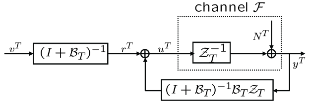
Figure 11: The block diagram of the CP structure for ISI Gaussian channel ${\mathcal{F}}$.

The capacity $C_{T}$ now takes the form

$$\begin{array}[]{lll}C_{T}({\mathcal{P}})&=&\displaystyle\sup\frac{1}{2(T+1)}\log\det K_{y}^{(T)}\\ &=&\displaystyle\sup\frac{1}{2(T+1)}\log\det\left({\mathcal{Z}}^{-1}_{T}(I+{\mathcal{B}}_{T})({\mathcal{Z}}_{T}{\mathcal{Z}}_{T}^{\prime}+K_{r}^{(T)})(I+{\mathcal{B}}_{T})^{\prime}{\mathcal{Z}}_{T}^{-1}{}^{\prime}\right)\\ &=&\displaystyle\sup\frac{1}{2(T+1)}\log\det({\mathcal{Z}}_{T}{\mathcal{Z}}_{T}^{\prime}+K_{r}^{(T)})\end{array}$$ (87)

where the supremum is over the power constraint

$$P_{T}:=\frac{1}{T+1}\textnormal{tr}({\mathcal{B}}_{T}{\mathcal{Z}}_{T}{\mathcal{Z}}_{T}^{\prime}{\mathcal{B}}_{T}^{\prime}+(I+{\mathcal{B}}_{T})K_{r}^{(T)}(I+{\mathcal{B}}_{T})^{\prime})\leq{\mathcal{P}}.$$ (88)

It is easily seen that the capacity in this form is identical to (82).

B-D Relation between the CP structure for ISI Gaussian channel and the general coding structure

We can establish correspondence relationship between the CP structure for ISI Gaussian channel ${\mathcal{F}}$ in Fig. 11 and the general coding structure for ${\mathcal{F}}$ in Fig. 2. In fact, the general coding structure for ${\mathcal{F}}$ in Fig. 2 was initially motivated by the CP structure for channel ${\mathcal{F}}$ in Fig. 11.

For any fixed $(K_{r}^{(T)},{\mathcal{B}}_{T})$ in the CP structure, define in the general coding structure that

$$\begin{array}[]{lll}{\mathcal{G}}_{T}&:=&(I+{\mathcal{B}}_{T})^{-1}{\mathcal{B}}_{T}{\mathcal{Z}}_{T}\\ A&:=&\Gamma_{0}^{-1}\left[\begin{tabular}[]{c|c}0&$I_{T}$\cr\hline\cr*&*\end{tabular}\right]\Gamma_{0}\;\;\in\mathbb{R}^{(T+1)\times(T+1)}\\ C&:=&\left[\matrix{1&0&\cdots&0}\right]\Gamma_{0},\end{array}$$ (89)

where $\Gamma_{0}:=(K_{r}^{(T)})^{\frac{1}{2}}$, and * can be any number. (Note that the case $K_{r}^{(T)}\geq 0$ but $K_{r}^{(T)}$ is not positive definite can be approached by a sequence of positive definite $K_{r}^{(T)}$, and thus it is sufficient to consider only positive definite $K_{r}^{(T)}$ in establishing the correspondence relation of the two structures.) Then it is easily verified that ${\mathcal{G}}_{T}$ is strictly lower triangular, $(A,C)$ is observable with a nonsingular observability matrix $\Gamma=\Gamma_{0}$, and $A$ can have eigenvalues not on the the unit circle and not at the locations of $F$’s eigenvalues. Therefore, for any given $(K_{r}^{(T)},{\mathcal{B}}_{T})$, we can find an admissible $(A,C,{\mathcal{G}}_{T})$, and it is straightforward to verify that they generate identical channel inputs $u^{T}$.

Conversely, for any fixed admissible $(A,C,{\mathcal{G}}_{T})$ with $\in\mathbb{R}^{(n+1)\times(n+1)}$, we can obtain an admissible $(K_{r}^{(T)},{\mathcal{B}}_{T})$ as

$$\begin{array}[]{lll}\\ {\mathcal{B}}_{T}&:=&{\mathcal{G}}_{T}{\mathcal{Z}}_{T}^{-1}(I-{\mathcal{G}}_{T}{\mathcal{Z}}_{T}^{-1})^{-1}\\ K_{r}^{(T)}&:=&\Gamma(A,C)\Gamma(A,C)^{\prime},\end{array}$$ (90)

which generates identical channel input $u^{T}$ as $(A,C,{\mathcal{G}}_{T})$ does.

As a result of the above reasoning, there is a corresponding relation between the CP structure for ${\mathcal{F}}$ and the general coding structure, and the maximum rate over all admissible $(K_{r}^{(T)},{\mathcal{B}}_{T})$ (namely $C_{T}$) equals that over all admissible $(A,C,{\mathcal{G}}_{T})$. In other words, we have

Lemma 1.

$$C_{T}({\mathcal{P}})=C_{T,T}({\mathcal{P}}).$$ (91)

Proof:

Note that $C_{T,T}$ is the maximum rate over all admissible $(A,C,{\mathcal{G}}_{T})$ with $\in\mathbb{R}^{(T+1)\times(T+1)}$. ∎

This lemma implies that the general coding structure with an extra constraint $T=n$ becomes the CP structure, that is, in the CP structure, the dimension of $A$ is equal to the horizon length. One advantage of considering the general coding structure is that we can allow $T\neq n$, which makes it possible to increase the horizon length to infinity without increasing the dimension of $A$, a crucial step towards the Kalman filtering characterization of the feedback communication problem.

Our study on the general coding structure also refines the CP structure. We can now identify more specific structure of the optimal $(K_{v}^{(T)},{\mathcal{B}}_{T})$. Indeed, we conclude that the CP structure needs to have a Kalman filter inside. We may further determine the optimal form of ${\mathcal{B}}_{T}$. From (90) and (32), we have that

$${\mathcal{B}}_{T}^{*}=-\widehat{\mathcal{G}}_{T}^{*}(A,C){\mathcal{Z}}_{T}^{-1}.$$ (92)

Therefore, to achieve $C_{T}$ in the CP structure, it is sufficient to search $(K_{v}^{(T)},{\mathcal{B}}_{T})$ in the form of

$$\begin{array}[]{lll}K_{v}^{(T)}&:=&(I-\widehat{\mathcal{G}}_{T}^{*}(A,C){\mathcal{Z}}_{T}^{-1})\Gamma(A,C)\Gamma(A,C)^{\prime}(I-\widehat{\mathcal{G}}_{T}^{*}(A,C){\mathcal{Z}}_{T}^{-1})^{\prime}\\ {\mathcal{B}}_{T}^{*}&:=&-\widehat{\mathcal{G}}_{T}^{*}(A,C){\mathcal{Z}}_{T}^{-1}.\end{array}$$ (93)

Additionally, as $T$ tends to infinity, it can be easily shown that $\{v_{t}\}$ is a stable process in order to achieve $C_{\infty}$.

B-E Proof of Proposition 4: Necessary condition for optimality

In this subsection, we show that our general coding structure, in the form of (42), satisfies the necessary condition for optimality as presented in Proposition 4.

Since $\{y_{t}\}$ is interchangeable with the innovations process $\{e_{t}\}$, in the sense that they determine each other causally and linearly, it suffices to show that $\mathbf{E}u_{t}e_{\tau}=0$. Note that

$$u_{t}=\mathbb{D}\mathbb{X}_{t}=\mathbb{D}\mathbb{A}\mathbb{X}_{t-1}-\mathbb{D}L_{t-1}e_{t-1},$$ (94)

and thus

$$\begin{array}[]{lll}\mathbf{E}u_{t}e_{t-1}&=&\mathbf{E}\mathbb{D}\mathbb{A}\mathbb{X}_{t-1}e_{t-1}-\mathbb{D}L_{t-1}K_{e,t-1}\\ &\stackrel{{\scriptstyle\textnormal{(a)}}}{{=}}&\mathbf{E}\mathbb{D}\mathbb{A}\mathbb{X}_{t-1}\mathbb{X}_{t-1}^{\prime}\mathbb{C}^{\prime}+\mathbf{E}\mathbb{D}\mathbb{A}\mathbb{X}_{t-1}N_{t-1}-\mathbb{D}\mathbb{A}\Sigma_{t-1}\mathbb{C}^{\prime}\\ &=&\mathbb{D}\mathbb{A}\Sigma_{t-1}\mathbb{C}^{\prime}+0-\mathbb{D}\mathbb{A}\Sigma_{t-1}\mathbb{C}^{\prime}=0,\end{array}$$ (95)

where (a) follows from (42) and (43). Similarly we can prove $\mathbf{E}u_{t}e_{\tau}=0$ for any $\tau<t-1$.

Appendix C Infinite-horizon: The properties of the general coding structure

C-A Proof of Proposition 5: Convergence to steady-state

In this subsection, we show that system (42) converges to a steady-state, as given by (51). To this aim, we first transform the Riccati recursion into a new coordinate system, then show that it converges to a limit, and finally prove that the limit is the unique stabilizing solution of the Riccati equation. The convergence to the steady-state follows immediately from the convergence of the Riccati recursion.

Consider a coordinate transformation given as

$$\underline{\mathbb{A}}:=\Phi\mathbb{A}\Phi^{-1}:=\left[\matrix{A&0\cr 0&F}\right],\;\;\underline{\mathbb{C}}:=\mathbb{C}\Phi^{-1},\;\;\underline{\Sigma}_{t}:=\Phi\underline{\Sigma}_{t}\Phi^{\prime},$$ (96)

where

$$\Phi:=\left[\matrix{I_{n+1}&0\cr-\phi&I_{m}}\right],$$ (97)

and $\phi$ is the unique solution to the Sylvester equation

$$F\phi-\phi A=-GC.$$ (98)

Note that the existence and uniqueness of $\phi$ is guaranteed by the assumption on $A$ that $\lambda_{i}(-A)+\lambda_{j}(F)\neq 0$ for any $i$ and $j$ (see Section IV-A).

This transformation transforms $\mathbb{A}$ into block-diagonal form with the unstable and stable eigenvalues in different blocks, and transforms the initial condition $\Sigma_{0}$ to

$$\underline{\Sigma}_{0}:=\Phi\left[\matrix{I_{n+1}&0\cr 0&0}\right]\Phi^{\prime}=\left[\matrix{I&-\phi^{\prime}\cr-\phi&\phi\phi^{\prime}}\right].$$ (99)

Therefore, the convergence of (44) with initial condition $\Sigma_{0}$ is equivalent to the convergence of

$$\underline{\Sigma}_{t+1}=\underline{\mathbb{A}}\underline{\Sigma}_{t}\underline{\mathbb{A}}^{\prime}-\frac{\underline{\mathbb{A}}\underline{\Sigma}_{t}\underline{\mathbb{C}}^{\prime}\underline{\mathbb{C}}\underline{\Sigma}_{t}\underline{\mathbb{A}}^{\prime}}{\underline{\mathbb{C}}\underline{\Sigma}_{t}\underline{\mathbb{C}}^{\prime}+1}$$ (100)

with initial condition $\underline{\Sigma}_{0}$. By [34], $\underline{\Sigma}_{t}$ would converge if

$$\det\left(\left[\matrix{0&0\cr 0&I_{m}}\right]-\underline{\Sigma}_{0}\left[\matrix{I_{n+1}&0\cr 0&X_{22}}\right]\right)\not=0,$$ (101)

where $X_{22}$ is a positive semi-definite matrix (whose value does not affect our result here). Since

$$\begin{array}[]{lll}\det\left(\left[\matrix{0&0\cr 0&I}\right]-\left[\matrix{I&-\phi^{\prime}\cr-\phi&\phi\phi^{\prime}}\right]\left[\matrix{I&0\cr 0&X_{22}}\right]\right)&=&\det\left(\left[\matrix{-I&\phi^{\prime}X_{22}\cr\phi&I-\phi\phi^{\prime}X_{22}}\right]\right)\\ &=&\det(-I)\det\left(I-\phi\phi^{\prime}X_{22}+\phi\phi^{\prime}X_{22}\right)\\ &\neq&0,\end{array}$$ (102)

we conclude that $\underline{\Sigma}_{t}$ converges to a limit $\underline{\Sigma}_{\infty}$.

This limit $\underline{\Sigma}_{\infty}$ is a positive semi-definite solution to

$$\underline{\Sigma}_{\infty}=\underline{\mathbb{A}}\underline{\Sigma}_{\infty}\underline{\mathbb{A}}^{\prime}-\frac{\underline{\mathbb{A}}\underline{\Sigma}_{\infty}\underline{\mathbb{C}}^{\prime}\underline{\mathbb{C}}\underline{\Sigma}_{\infty}\underline{\mathbb{A}}^{\prime}}{\underline{\mathbb{C}}\underline{\Sigma}_{\infty}\underline{\mathbb{C}}^{\prime}+1}.$$ (103)

By [31], (103) has a unique stabilizing solution because $(\underline{\mathbb{A}},\underline{\mathbb{C}})$ is observable and $\underline{\mathbb{A}}$ does not have any eigenvalues on the unit circle. Therefore, $\underline{\Sigma}_{\infty}$ is this unique stabilizing solution, which can be computed from (103) as (see also [34])

$$\underline{\Sigma}_{\infty}=\left[\matrix{\underline{\Sigma}_{11}&0\cr 0&0}\right]$$ (104)

where $\underline{\Sigma}_{11}$ is the positive-definite solution to a reduced order Riccati equation

$$\underline{\Sigma}_{11}=A\underline{\Sigma}_{11}A^{\prime}-\frac{A\underline{\Sigma}_{11}(C+H\phi)^{\prime}(C+H\phi)\underline{\Sigma}_{11}A^{\prime}}{(C+H\phi)\underline{\Sigma}_{11}(C+H\phi)^{\prime}+1}.$$ (105)

and has rank $(n+1)$ (cf. [34]). Thus, $\Sigma_{t}$ converges to

$$\Sigma_{\infty}=\left[\matrix{\underline{\Sigma}_{11}&\underline{\Sigma}_{11}\phi^{\prime}\cr\phi\underline{\Sigma}_{11}&\phi\underline{\Sigma}_{11}\phi^{\prime}}\right]$$ (106)

with rank $(n+1)$.

C-B Infinite-horizon feedback capacities

If the noise in the colored Gaussian channel forms a (an asymptotic) stationary process, then $C_{T}({\mathcal{P}})$ has a finite limit (cf. [15]; the proof utilizes the superadditivity of $C_{T}$, similar to the case of forward communication capacities studied in [36]), which also has the operational and information meanings. Therefore, we have

$$\lim_{T\rightarrow\infty}C_{T}=C_{\infty}<\infty,$$ (107)

where $C_{\infty}$ is the operational or information infinite-horizon capacity (cf. [6, 11]).

By Lemma 1, the above implies that

$$\lim_{T\rightarrow\infty}C_{T,T}=C_{\infty}.$$ (108)

Note that this does not simply lead to that $\lim_{n\rightarrow\infty}\lim_{T\rightarrow\infty}C_{T,n}=C_{\infty}$ or $C_{\infty}=C^{s}$, since we could not show that the involved limits (including taking the supremum) are interchangeable in this case.

Appendix D Proof of Proposition 7: $K_{\mathcal{E}}=0$

In this section, we prove that $K_{\mathcal{E}}$ has to be 0 to ensure the optimality in (62).

We first derive some properties of the communication system using the stationary GM inputs and the steady-state Kalman filtering. The system dynamics is given by

$$\left\{\begin{array}[]{lll}u_{t}&=&d^{\prime}\tilde{s}_{s,t}+{\mathcal{E}}_{t}\\ s_{t+1}&=&Fs_{t}+Gu_{t}\\ y_{t}&=&Hs_{t}+N_{t}+u_{t}\\ \tilde{s}_{s,t+1}&=&s_{t}-\hat{s}_{s,t}\\ \hat{s}_{s,t+1}&=&F\hat{s}_{s,t}+L_{s}e_{t}\\ e_{t}&=&y_{t}-H\hat{s}_{s,t}=(H+d^{\prime})\tilde{s}_{s,t}+{\mathcal{E}}_{t}+N_{t}\\ \tilde{s}_{s,t+1}&=&F\tilde{s}_{s,t}+Gu_{t}-L_{s}e_{t},\end{array}\right.$$ (109)

where $\hat{s}_{s,0}=0$ and $\tilde{s}_{s,0}=0$. As before, the Kalman filter innovations $\{e_{t}\}$ will play an important role. The innovations process is white with variance asymptotically equal to

$$K_{e}=1+K_{{\mathcal{E}}}+(H+d^{\prime})\Sigma_{s}(H+d^{\prime})^{\prime},$$ (110)

where $\Sigma_{s}:=\mathbf{E}\tilde{s}_{s}\tilde{s}_{s}^{\prime}$. Following the same derivation for Proposition 6, we know that the asymptotic information rate is given by

$$I({\mathcal{E}};y)=\frac{1}{2}\log K_{e},$$ (111)

which is consistent with the result in [12].

We now invoke the equivalence between the colored Gaussian channel and the ISI channel ${\mathcal{F}}$, that is, instead of generating $y$ by (109), we generate $y$ by

$$\left\{\begin{array}[]{lll}\tilde{y}_{t}&=&u_{t}+Z_{t}\\ s_{c,t+1}&=&Fs_{c,t}+G\tilde{y}_{t}\\ y_{t}&=&Hs_{c,t}+\tilde{y}_{t},\end{array}\right.$$ (112)

where $s_{c,0}=0$. Since $Z^{T}={\mathcal{Z}}_{T}N^{T}$, the mapping from $(u,N)$ to $y$ here is equivalent to that in (109). Therefore, (109) becomes

$$\left\{\begin{array}[]{lll}u_{t}&=&d^{\prime}\tilde{s}_{s,t}+{\mathcal{E}}_{t}\\ \tilde{y}_{t}&=&u_{t}+Z_{t}\\ s_{c,t+1}&=&Fs_{c,t}+G\tilde{y}_{t}\\ y_{t}&=&Hs_{c,t}+\tilde{y}_{t}\\ \hat{s}_{s,t+1}&=&F\hat{s}_{s,t}+L_{s}e_{t}\\ e_{t}&=&y_{t}-H\hat{s}_{s,t}=(H+d^{\prime})\tilde{s}_{s,t}+{\mathcal{E}}_{t}+N_{t}\\ \tilde{s}_{s,t+1}&=&F\tilde{s}_{s,t}+Gu_{t}-L_{s}e_{t},\end{array}\right.$$ (113)

where $\hat{s}_{s,0}=0$; see Fig. 12 for the block diagram.

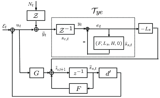
Figure 12: Block diagram for the communication system using the GM inputs and Kalman filtering, where $s_{c,t}$ is the state for ${\mathcal{Z}}^{-1}$ with $s_{c,0}=0$, and $\hat{s}_{s,t}$ is the state for system $(F,L_{s},H,0)$ with $\hat{s}_{s,0}=0$.

Our analysis of this system is facilitated by considering transfer functions. Note that

$$\begin{array}[]{lll}{\mathcal{T}}_{{\mathcal{E}}u}&=&\mathbb{S}\\ {\mathcal{T}}_{Nu}&=&\mathbb{T}{\mathcal{Z}},\end{array}$$ (114)

where $\mathbb{S}$ is the sensitivity, and $\mathbb{T}:=\mathbb{S}-1$ is the complimentary sensitivity. (The sensitivity $\mathbb{S}$ here should not be confused with the sensitivity in Section V-A.) Then we have

$$\begin{array}[]{lll}u&=&\mathbb{S}{\mathcal{E}}+\mathbb{T}{\mathcal{Z}}N\\ \tilde{y}&=&\mathbb{S}({\mathcal{E}}+{\mathcal{Z}}N).\end{array}$$ (115)

Now assume that $d$ and $K_{\mathcal{E}}$ form the optimal solution to (62), where $K_{\mathcal{E}}\neq 0$, for contradiction purpose. We can then compute the corresponding optimal $\Sigma_{s}$, $L_{s}$, $\mathbb{S}$, $\mathbb{T}$, etc. Fix the optimal $L_{s}$, $\mathbb{S}$, and $\mathbb{T}$. We will show that this leads to: 1) The whiteness of $\{\tilde{y}_{t}\}$; 2) $L_{s}=G$; 3) $K_{\mathcal{E}}=0$ and hence contradiction.

1) For fixed optimal values of $L_{s}$, $\mathbb{S}$, and $\mathbb{T}$, suppose that we can have the freedom of choosing the power spectrum of ${\mathcal{E}}$ in (113). Since we have assumed the optimality of a white process $\{{\mathcal{E}}_{t}\}$, it must hold that any correlated process $\{{\mathcal{E}}_{c,t}\}$ does not lead to a larger mutual information than $\{{\mathcal{E}}_{t}\}$ does. Precisely, assume a stationary correlated process $\{{\mathcal{E}}_{c,t}\}$ replaces the white process $\{{\mathcal{E}}_{t}\}$ in (113). Then $\{{\mathcal{E}}_{t}\}$ yields the maximum achievable rate over all possible $\{{\mathcal{E}}_{c,t}\}$, i.e., it solves

$$\begin{array}[]{cl}&\displaystyle{\max_{L_{s},\mathbb{S},\mathbb{T}\textrm{ \small fixed},{\mathcal{S}}_{{\mathcal{E}}_{c}}(e^{j2\pi\theta})}}\displaystyle I({\mathcal{E}}_{c};\tilde{y}).\\ &{}^{s.t.\>\mathbf{E}u^{2}\leq{\mathcal{P}}}\end{array}$$ (116)

Since

$$I({\mathcal{E}}_{c};\tilde{y})=h(\tilde{y})-h(\tilde{y}|{\mathcal{E}}_{c})=h(\tilde{y})-h(\mathbb{S}{\mathcal{Z}}N)$$ (117)

and $h(\mathbb{S}{\mathcal{Z}}N)$ is fixed for fixed $\mathbb{S}$, the above optimization is equivalent to

$$\begin{array}[]{cl}&\displaystyle{\max_{{\mathcal{S}}_{{\mathcal{E}}_{c}}(e^{j2\pi\theta})}}\displaystyle\frac{1}{2}\displaystyle\int_{-\frac{1}{2}}^{\frac{1}{2}}\log{\mathcal{S}}_{\tilde{y}}(e^{j2\pi\theta})d\theta.\\ &{}^{s.t.\>\mathbf{E}u^{2}=\int_{-\frac{1}{2}}^{\frac{1}{2}}{\mathcal{S}}_{\mathbb{S}}(e^{j2\pi\theta}){\mathcal{S}}_{{\mathcal{E}}_{c}}(e^{j2\pi\theta})+{\mathcal{S}}_{\mathbb{T}}(e^{j2\pi\theta}){\mathcal{S}}_{{\mathcal{Z}}}(e^{j2\pi\theta})d\theta\leq{\mathcal{P}}}\end{array}$$ (118)

However, this optimization problem is equivalent to solving, for some ${\mathcal{P}}_{1}\geq 0$,

$$\begin{array}[]{cl}&\displaystyle{\max_{{\mathcal{S}}_{{\mathcal{E}}_{c}}(e^{j2\pi\theta})}}\displaystyle\frac{1}{2}\displaystyle\int_{-\frac{1}{2}}^{\frac{1}{2}}\log\left({\mathcal{S}}_{\mathbb{S}}(e^{j2\pi\theta}){\mathcal{S}}_{{\mathcal{E}}_{c}}(e^{j2\pi\theta})+{\mathcal{S}}_{\mathbb{S}}(e^{j2\pi\theta}){\mathcal{S}}_{{\mathcal{Z}}}(e^{j2\pi\theta})\right)d\theta,\\ &{}^{s.t.\>\int_{-\frac{1}{2}}^{\frac{1}{2}}{\mathcal{S}}_{\mathbb{S}}(e^{j2\pi\theta}){\mathcal{S}}_{{\mathcal{E}}_{c}}(e^{j2\pi\theta})d\theta\leq{\mathcal{P}}_{1}}\end{array}$$ (119)

which we identify as a new forward communication problem, see Fig. 13. In this problem, we want to tune the power spectrum of $\mathbb{S}{\mathcal{E}}_{c}$, the effective channel input, to get the maximum rate. The optimal solution is given by waterfilling, namely, the power spectrum ${\mathcal{S}}_{\mathbb{S}}(e^{j2\pi\theta}){\mathcal{S}}_{{\mathcal{E}}_{c}}(e^{j2\pi\theta})$ needs to waterfill the power spectrum ${\mathcal{S}}_{\mathbb{S}}(e^{j2\pi\theta}){\mathcal{S}}_{{\mathcal{Z}}}(e^{j2\pi\theta})$. By optimality of $\{{\mathcal{E}}_{t}\}$, $K_{\mathcal{E}}{\mathcal{S}}_{\mathbb{S}}(e^{j2\pi\theta})$ is the waterfilling solution.

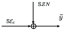
Figure 13: An equivalent forward communication channel. Here $\mathbb{S}{\mathcal{E}}_{c}$ is the effective input, $\mathbb{S}{\mathcal{Z}}N$ is the effective channel noise, and $\tilde{y}$ is the output.

Since ${\mathcal{S}}_{\mathbb{S}}(e^{j2\pi\theta})=0$ for some $\theta$ if and only if $\mathbb{S}(z)$ has a zero for that $\theta$ on the unit circle, and since $\mathbb{S}(z)$ is a finite dimension transfer function with a finite number of zeros, the power spectrum ${\mathcal{S}}_{\mathbb{S}}(e^{j2\pi\theta})$ cannot have zero amplitude at any interval. This follows that the support of the channel input spectrum $K_{\mathcal{E}}{\mathcal{S}}_{\mathbb{S}}(e^{j2\pi\theta})$ is $[-1/2,1/2]$.

In waterfilling, if the support of input spectrum is $[-1/2,1/2]$, then the output spectrum must be flat. This is easily proven by contradiction. Thus, $\{\tilde{y}_{t}\}$ is a white process. Let us assume that its variance is $\sigma^{2}$.

2) Note that both $\tilde{y}$ and $e$ have white spectrum, which imposes condition on the choice of $L_{s}$. The transfer function ${\mathcal{T}}_{ye}$ is illustrated in Fig. 14, where we can see that its structure is a Kalman filter structure. To make $e$ white, it is necessary to choose $L_{s}$ to be the Kalman filter gain (cf. [31]), given by

$$L_{s}:=\frac{F\Sigma_{c}H^{\prime}+\sigma^{2}G}{H\Sigma_{c}H^{\prime}+\sigma^{2}},$$ (120)

where $\Sigma_{c}$ is the estimation error covariance matrix and is a nonnegative solution to the Riccati equation

$$\Sigma_{c}=F\Sigma_{c}F^{\prime}+\sigma^{2}GG^{\prime}-\frac{(F\Sigma_{c}H^{\prime}+\sigma^{2}G)(F\Sigma_{c}H^{\prime}+\sigma^{2}G)^{\prime}}{H\Sigma_{c}H^{\prime}+\sigma^{2}}.$$ (121)

Clearly, $\Sigma_{c}=0$ is a solution to the Riccati equation. By [31], it is also the unique nonnegative solution. Hence, we need to choose $L_{s}:=G$.

Figure 14: The state-space representation of the transfer function ${\mathcal{T}}_{ye}$.

3) The fact that $L_{s}=G$ leads to reduction of system (113) or equivalently (109). We have

$$\begin{array}[]{lll}\tilde{s}_{t+1}&=&(F-GH)\tilde{s}_{t}-GN_{t}\\ \Sigma_{s}&=&(F-GH)\Sigma_{s}(F-GH)^{\prime}+GG^{\prime}.\end{array}$$ (122)

In the case that $(F-GH)$ is unstable, the closed-loop of (113) is unstable and cannot transmit information. In the case that $(F-GH)$ is stable, the steady-state of $\Sigma_{s}$ depends only on $(F,G,H)$ and is independent of the choice of $d$ and $K_{\mathcal{E}}$, and thus (62) becomes

$$\begin{array}[]{cl}C_{\infty}=&\displaystyle{\max_{\Sigma_{s}\textrm{ \small fixed},d\in\mathbb{R}^{m},K_{\mathcal{E}}\in\mathbb{R}}}\displaystyle\frac{1}{2}\log(1+K_{\mathcal{E}}+(H+d^{\prime})\Sigma_{s}(H+d^{\prime})^{\prime}).\\ &{}^{s.t.\>{\mathcal{P}}=d^{\prime}\Sigma_{s}d+K_{\mathcal{E}}}\end{array}$$ (123)

This is equivalent to

$$\begin{array}[]{cl}&\displaystyle{\max_{d\in\mathbb{R}^{m},K_{\mathcal{E}}\in\mathbb{R}}}\displaystyle H\Sigma_{s}d,\\ &{}^{s.t.\>d^{\prime}\Sigma_{s}d\leq{\mathcal{P}}-K_{\mathcal{E}}}\end{array}$$ (124)

which requires $K_{\mathcal{E}}=0$.

Appendix E Optimality of the proposed coding scheme

E-A Proof of Proposition 8: Finite dimensionality of the optimal scheme

i) To show that $C_{\infty,n}$ is non-decreasing as $n$ increases, note that, an encoder $(A,C)$ of dimension $(n+1)$ can be arbitrarily approximated by a sequence of encoders $\{(A_{i},C_{i})\}$ of dimension $(n+2)$ in the form of

$$\left(\left[\begin{array}[]{c|c}A&0\cr\hline\cr 0&1\end{array}\right],\left[\begin{array}[]{c|c}C&\frac{1}{i}\end{array}\right]\right),$$ (125)

and therefore the supremum in (64) with encoder dimension $(n+2)$ is no smaller than the supreme with encoder dimension $(n+1)$. So $C_{\infty,n}$ is increasing in $n$.

ii) By proposition 6 and the definition for $C_{\infty,m-1}({\mathcal{P}})$, the optimization problem for solving $C_{\infty,m-1}({\mathcal{P}})$ is given by

$$\begin{array}[]{lcl}C_{\infty,m-1}({\mathcal{P}})=&\displaystyle\sup_{A\in\mathbb{R}^{m\times m},C}&\displaystyle\frac{1}{2}\log(\mathbb{C}\Sigma\mathbb{C}^{\prime}+1)\\ &{}^{s.t.\Sigma=\mathbb{A}\Sigma\mathbb{A}^{\prime}-\mathbb{A}\Sigma\mathbb{C}^{\prime}(\mathbb{C}\Sigma\mathbb{C}^{\prime}+1)^{-1}\mathbb{C}\Sigma\mathbb{A}^{\prime}}\\ &\;\;{}^{\mathbb{D}\Sigma\mathbb{D}^{\prime}={\mathcal{P}}}\end{array}$$ (126)

To compare it with $C_{\infty}({\mathcal{P}})$, we rewrite (62) and (63) in another form, incorporating $K_{\mathcal{E}}=0$. Define

$$\begin{array}[]{lll}\bar{\mathbb{A}}&:=&\left[\begin{array}[]{c | c}F+Gd^{\prime}&0\\ \hline\cr Gd^{\prime}&F\end{array}\right]\\ \bar{\mathbb{C}}&:=&[d\quad H]\\ \bar{\mathbb{D}}&:=&[d\quad 0]\\ \bar{\Sigma}&:=&\left[\begin{array}[]{c | c}\Sigma_{s}&\Sigma_{s}\\ \hline\cr\Sigma_{s}&\Sigma_{s}\end{array}\right].\end{array}$$ (127)

It is then straightforward to verify that

$$\begin{array}[]{rcl}\displaystyle\frac{1}{2}\log(1+(H+d^{\prime})\Sigma_{s}(H+d^{\prime})^{\prime})&=&\displaystyle\frac{1}{2}\log(1+\bar{\mathbb{C}}\bar{\Sigma}\bar{\mathbb{C}}^{\prime})\\ d^{\prime}\Sigma_{s}d&=&\bar{\mathbb{D}}\bar{\Sigma}\bar{\mathbb{D}}^{\prime}\\ \displaystyle\bar{\mathbb{A}}\bar{\Sigma}\bar{\mathbb{A}}^{\prime}-\bar{\mathbb{A}}\bar{\Sigma}\bar{\mathbb{C}}^{\prime}(\bar{\mathbb{C}}\bar{\Sigma}\bar{\mathbb{C}}^{\prime}+1)^{-1}\bar{\mathbb{C}}\bar{\Sigma}\bar{\mathbb{A}}^{\prime}&=&\bar{\Sigma},\end{array}$$ (128)

which yields that

$$\begin{array}[]{lcl}C_{\infty}({\mathcal{P}})=&\displaystyle{\sup_{d\in\mathbb{R}^{m}}}&\displaystyle\frac{1}{2}\log(1+\bar{\mathbb{C}}\bar{\Sigma}\bar{\mathbb{C}}^{\prime})\\ &{}_{s.t.\bar{\Sigma}=\bar{\mathbb{A}}\bar{\Sigma}\bar{\mathbb{A}}^{\prime}-\bar{\mathbb{A}}\bar{\Sigma}\bar{\mathbb{C}}^{\prime}(\bar{\mathbb{C}}\bar{\Sigma}\bar{\mathbb{C}}^{\prime}+1)^{-1}\bar{\mathbb{C}}\bar{\Sigma}\bar{\mathbb{A}}^{\prime}}\\ &\;\;{}_{\bar{\mathbb{D}}\bar{\Sigma}\bar{\mathbb{D}}^{\prime}={\mathcal{P}}}\end{array}$$ (129)

Comparing (129) with (126), we conclude that $C_{\infty,m-1}({\mathcal{P}})\geq C_{\infty}({\mathcal{P}})$. However, since for each $(A,C)$, the channel input sequence is stationary by the steady-state characterization of the general coding structure, it holds that $C_{\infty,m-1}({\mathcal{P}})\leq C_{\infty}({\mathcal{P}})$. Therefore, we have

$$C_{\infty,m-1}({\mathcal{P}})=C_{\infty}({\mathcal{P}}).$$ (130)

Then ii) follows from i) immediately.

E-B Proof of Proposition 9: Achieving $C_{\infty}$ in the information sense

By Proposition 8, the optimization problem for solving $P_{\infty}({\mathcal{R}})$ in (9) (which is equivalent to solving $C_{\infty}({\mathcal{P}})$) can be reformulated as

$$\begin{array}[]{lcl}[A^{opt},C^{opt},\Sigma^{opt}]:=&\displaystyle{\textnormal{arg}\inf_{A\in\mathbb{R}^{m\times m},C}}&\mathbb{D}\Sigma\mathbb{D}^{\prime},\\ &{}^{s.t.\Sigma=\mathbb{A}\Sigma\mathbb{A}^{\prime}-\mathbb{A}\Sigma\mathbb{C}^{\prime}(\mathbb{C}\Sigma\mathbb{C}^{\prime}+1)^{-1}\mathbb{C}\Sigma\mathbb{A}^{\prime}}\\ &\;\;{}^{\log DI(A)={\mathcal{R}}}\end{array}$$ (131)

for any desired rate ${\mathcal{R}}$. Without loss of generality, we may assume that $(A,C)$ is in the observable canonical form, i.e.

$$\begin{array}[]{lll}A:=\left[\begin{array}[]{c|c}0_{n\times 1}&I_{n}\cr\hline\cr a_{n}&a_{n-1}\cdots a_{1}\end{array}\right]\\ C:=\left[\begin{array}[]{cc}1&0_{1\times n}\end{array}\right].\end{array}$$ (132)

Observe that $\det A=a_{n}$. Thus, $DI(A)=|\det A|=|a_{n}|$ if $A$ does not contain stable eigenvalues, and $DI(A)>|\det A|=|a_{n}|$ otherwise.

As a consequence, if we search over $A$ with $a_{n}$ fixed to be $2^{\mathcal{R}}$ or $-2^{\mathcal{R}}$, we actually enforce $DI(A)\geq 2^{R}$. However, the optimal solution must satisfy $DI(A^{opt})=2^{\mathcal{R}}$, since otherwise the system has a rate equal to $R_{\infty,m-1}=\log DI(A^{opt})>{\mathcal{R}}$, which would require more power than the case that $R_{\infty,m-1}={\mathcal{R}}$; notice that (131) is a power minimization problem. To summarize, we can remove the constraint $\log DI(A)={\mathcal{R}}$ by letting $a_{n}=\pm 2^{\mathcal{R}}$ in (132), and the optimal solution $A$ does not contain stable eigenvalues. Furthermore, note that unit-circle eigenvalues do not generate any rate or power and hence can be removed. Thus, if $A^{opt}$ has $(n^{*}+1)$ unstable eigenvalues, we can solve the optimization problem with $A$ having size $(n^{*}+1)$ and the obtained optimal solution still achieves $C_{\infty}$.

E-C Proof of Proposition 10: Optimality in the analog transmission

The end-to-end distortion is given by

$$\begin{array}[]{lll}\mbox{MSE}(\hat{W}_{t})&=&\mathbf{E}(W-\hat{W}_{t})(W-\hat{W}_{t})^{\prime}\\ &=&\mathbf{E}(x_{0}-\hat{x}_{0,t})(x_{0}-\hat{x}_{0,t})^{\prime}\\ &=&\mathbf{E}(A^{-t-1}x_{t+1}-A^{-t-1}\hat{x}_{t+1})(A^{-t-1}x_{t+1}-A^{-t-1}\hat{x}_{t+1})^{\prime}\\ &=&\mathbf{E}A^{-t-1}\tilde{x}_{t+1}\tilde{x}_{t+1}^{\prime}A^{\prime}{}^{-t-1}\\ &=&A^{-t-1}\Sigma_{x,t+1}A^{\prime}{}^{-t-1},\end{array}$$ (133)

where

$$\Sigma_{x,t+1}:=[I,0]\Sigma_{t+1}[I,0]^{\prime}$$ (134)

and the expectation is w.r.t. the randomness in $W$ and $\hat{W}_{t}$. By rate-distortion theory, the above distortion needs an asymptotic rate $R$ satisfying

$$\begin{array}[]{lll}R&\geq&\displaystyle\lim_{t\rightarrow\infty}\frac{1}{2(t+1)}\log\frac{{\mathcal{P}}^{n^{*}+1}}{\det MSE(\hat{W}_{t})}\\ &=&\displaystyle\lim_{t\rightarrow\infty}\frac{1}{2(t+1)}\log\frac{\det A^{2t+2}}{\det\Sigma_{x,t+1}}\\ &=&\displaystyle\log|\det A|.\end{array}$$ (135)

From Proposition 9, we know that $\log|\det A^{*}|$ equals $C_{\infty}$ and the average channel input power equals ${\mathcal{P}}$. Because $C_{\infty}$ is the supremum of asymptotic rate, it follows that the equality in (135) is achieved. Then we see that the proposition holds.

E-D Proof of Proposition 11: Optimality in digital transmission

It is sufficient to show that $R_{\infty,n}(A,C)$ is achievable for any fixed $(A,C)$. To show this, for the fixed $(A,C)$, construct the scheme in Fig. 2 and use ${\mathcal{G}}_{T}^{*}$, the Kalman-filter based optimal receiver. The closed-loop (42) is stabilized and will converge to its steady-state for large enough $T$.

We can then directly verify that Theorems 4.3 and 4.6 in [14] are applicable to the (steady-state) LTI system. These theorems assert that, if the closed-loop system is stabilized, then we can construct a sequence of codes to reliably (in the sense of vanishing probability of error) transmit the initial conditions associated with the open-loop unstable eigenvalues of $A$ (denoted $a_{0},\cdots,a_{k}$, if any), at a rate

$$R:=(1-\epsilon)R_{\infty,n}(A,C)$$ (136)

for any $\epsilon>0$, and in the meantime, $P_{\infty,n}(A,C)\leq\mathcal{P}$ holds. Therefore, we conclude that, for any $(A,C)$, the portion of $W$ that is associated with the unstable eigenvalues of $A$ is transmitted reliably from the transmitter to the receiver at rate arbitrarily close to $R_{\infty,n}(A,C)$. Moreover, we notice that we can achieve $C_{\infty,n}$ by a sequence of purely unstable $(A,C)$ (i.e. $k=n$), in which the initial condition $W$ is the message being transmitted. This follows that $W$ is transmitted at the capacity rate.

In addition, [14] showed that for any choice of $x_{0}$, it holds that

$$PE_{T}=1-\prod_{i=0}^{n}\left(1-2Q\left(\frac{\sigma_{T,i}^{-{\epsilon}}}{2}\right)\right),$$ (137)

where $\sigma_{T,i}$ is the square root of the $i$th eigenvalue of $\mbox{MSE}(\hat{x}_{0,T})$, and

$$\begin{array}[]{lll}\mbox{MSE}(\hat{x}_{0,T})&=&\mathbf{E}(x_{0}-\hat{x}_{0,T})(x_{0}-\hat{x}_{0,T})^{\prime}\\ &=&A^{-T-1}\Sigma_{x,T+1}A^{\prime}{}^{-T-1}.\end{array}$$ (138)

Note that the expectation is w.r.t. the randomness in $\hat{x}_{0,T}$ only, different from (133), and that asymptotically $\Sigma_{t+1}$ and hence $\Sigma_{x,T+1}$ are independent on the choice of $x_{0}$.

It then holds for each $i$,

$$\begin{array}[]{lll}(\sigma_{T,i})^{2}&\leq&\lambda_{\max}(\mbox{MSE}(\hat{x}_{0,T}))\\ &=&\lambda_{\max}(A^{-T-1}\Sigma_{x,T+1}A^{\prime}{}^{-T-1})\\ &\stackrel{{\scriptstyle\textnormal{(a)}}}{{=}}&\lambda_{\max}(A^{\prime}{}^{-T-1}A{}^{-T-1}\Sigma_{x,T+1})\\ &\stackrel{{\scriptstyle\textnormal{(b)}}}{{\leq}}&\bar{\sigma}(A^{\prime}{}^{-T-1}A{}^{-T-1}\Sigma_{x,T+1})\\ &\stackrel{{\scriptstyle\textnormal{(c)}}}{{\leq}}&\bar{\sigma}(A^{\prime}{}^{-T-1}A{}^{-T-1})\bar{\sigma}(\Sigma_{x,T+1})\\ &=&\left(\bar{\sigma}(A^{\prime}A)\right)^{-T-1}\bar{\sigma}(\Sigma_{x,T+1})\end{array}$$ (139)

where $\lambda_{\max}(M)$ denotes the maximum eigenvalue of $M$, $\bar{\sigma}(M)$ denotes the maximum singular value of $M$, (a) follows from $\lambda(AB)=\lambda(BA)$, (b) follows from $|\lambda(A)|\leq\bar{\sigma}(A)$, and (c) is because the maximum singular value is an induced norm. Since $\Sigma_{x,T+1}$ converges to steady-state value exponentially, the above implies that, for $T$ large enough, each $\sigma_{T,i}$ decays to zero exponentially as $T$ increases.

Now using the union bound and the Chernoff bound, we have

$$\begin{array}[]{lll}PE_{T}&\leq&\displaystyle\sum_{i=0}^{n}2Q\left(\frac{\sigma_{T,i}^{-{\epsilon}}}{2}\right)\\ &\leq&\displaystyle\sum_{i=0}^{n}\frac{4}{\sqrt{2\pi}\sigma_{T,i}^{-{\epsilon}}}\exp\left(-\frac{\sigma_{T,i}^{-2{\epsilon}}}{8}\right),\end{array}$$ (140)

and hence $PE_{T}$ decreases to zero doubly exponentially since ${\epsilon}>0$ and $\sigma_{T,i}$ decays exponentially. Thus we prove the proposition.

ACKNOWLEDGEMENTS

The authors would like to thank Anant Sahai, Sekhar Tatikonda, Sanjoy Mitter, Zhengdao Wang, Murti Salapaka, Shaohua Yang, Donatello Materassi, and Young-Han Kim for useful discussion.

References

- [1] J.P.M. Schalkwijk and T. Kailath. A coding scheme for additive noise channels with feedback Part I: No bandwidth constraint. IEEE Trans. Inform. Theory, IT-12:172–182, Apr. 1966.
- [2] J.P.M. Schalkwijk. A coding scheme for additive noise channels with feedback Part II:Bandlimited signals. IEEE Trans. Inform. Theory, IT-12(2):183–189, Apr. 1966.
- [3] J. K. Omura. Optimum linear transmission of analog data for channels with feedback. IEEE Trans. Inform. Theory, 14(1):38–43, Jan. 1968.
- [4] S.A. Butman. A general formulation of linear feedback communication systems with solutions. IEEE Trans. Inform. Theory, IT-15:392–400, 1969.
- [5] S.A. Butman. Linear feedback rate bounds for regressive channels. IEEE Trans. Inform. Theory, IT-22:363–366, 1976.
- [6] T.M. Cover and S. Pombra. Gaussian feedback capacity. IEEE Trans. Inform. Theory, IT-35:37–43, 1989.
- [7] L.H. Ozarow. Random coding for additive Gaussian channels with feedback. IEEE Trans. Inform. Theory, 36(1):17–22, Jan. 1988.
- [8] K. Yanagi. Necessary and sufficient condition for capacity of the discrete-time Gaussian channel to be increased by feedback. IEEE Trans. Inform. Theory, 38:1788–1791, Nov. 1992.
- [9] E. Ordentlich. A class of optimal coding schemes for moving average additive Gaussian noise channels with feedback. Proc. IEEE International Symposium on Information Theory (ISIT), page 467, June 1994.
- [10] A. Shahar-Doron and M. Feder. On a capacity achieving scheme for the colored Gaussian channel with feedback. Proc. 2004 IEEE International Symposium on Information Theory (ISIT), page 74, July 2004.
- [11] S. Tatikonda and S. Mitter. The capacity of channels with feedback Part I: the General Case. Submitted to IEEE Trans. Inform. Theory, 2001.
- [12] S. Yang, A. Kavcic, and S. Tatikonda. Feedback capacity of power constrained Gaussian channels with memory. Submitted to IEEE Trans. Inform. Theory, 2003.
- [13] A. Sahai. Anytime Information Theory. PhD thesis, MIT, Cambridge, MA, 2001.
- [14] N. Elia. When Bode meets Shannon: Control-oriented feedback communication schemes. IEEE Trans. Autom. Contr., 49(9):1477–1488, Sept. 2004.
- [15] Young-Han Kim. The feedback capacity of the first-order moving average Gaussian channel. http://arxiv.org/abs/cs/0411036, Nov. 2004.
- [16] Young-Han Kim. On the feedback capacity of stationary Gaussian channels. Proc. 43rd Annual Allerton Conference on Communication, Control, and Computing, Sept. 2005.
- [17] J. Massey. Causality, feedback, and directed information. Proc. IEEE International Symposium on Information Theory and Applications (ISITA), pages 303–305, 1990.
- [18] L. H. Ozarow. The capacity of the white Gaussian multiple access channel with feedback. IEEE Trans. Inform. Theory, 30:623–629, 1984.
- [19] G. Kramer. Feedback strategies for white Gaussian interference networks. IEEE Trans. Inform. Theory, 48(6):1423–1438, June 2002.
- [20] J. Liu, N. Elia, and S. Tatikonda. Capacity-achieving feedback scheme for Markov channels with channel state information. Submitted to IEEE Trans. Inform. Theory, Aug. 2005.
- [21] F. R. Kschischang, B. J. Frey, and H. A. Loeliger. Factor graphs and the sum-product algorithm. IEEE Trans. Inform. Theory, 47(2):498 – 519, Feb. 2001.
- [22] G. D. Forney. On the role of MMSE estimation in approaching the information theoretic limits of linear Gaussian channels: Shannon meets Wiener. Proc. 41st Annual Allerton Conference on Communication, Control, and Computing, Oct. 2003.
- [23] S. Yang, A. Kavcic, and S. Tatikonda. Feedback capacity of finite-state machine channels. Submitted to IEEE Trans. Inform. Theory, 51(3):799–810, Mar. 2005.
- [24] S. K. Mitter and N. Newton. Information and entropy flow in the Kalman-Bucy filter. J. of Stat. Phys., 118:145–176, Jan. 2005.
- [25] D. Guo, S. Shamai, and S. Verdu. Mutual information and minimum mean-square error in Gaussian channels. IEEE Trans. Inform. Theory, 51(4):1261–1282, Apr. 2005.
- [26] A. Papoulis and S. U. Pillai. Probability, Random Variables and Stochastic Processes. McGraw-Hill, Boston, MA, 4th edition, 2002.
- [27] S. Tatikonda. Control Under Communication Constraints. PhD thesis, MIT, Cambridge, MA, Aug. 2000.
- [28] M. Gastpar. On remote sources and channels with feedback. Proc. 38th Annual Conference on Information Sciences and Systems (CISS), 2004.
- [29] S. Tatikonda and S. Mitter. Control over noisy channels. IEEE Trans. Autom. Contr., 49(7):1196 – 1201, July 2004.
- [30] S. M. Kay. Fundamentals of Statistical Signal Processing I: Estimation Theory. Prentice-Hall PTR, Englewood Cliffs, N.J., 1998.
- [31] T. Kailath, A. Sayed, and B. Hassibi. Linear Estimation. Prentice Hall, 2000, Englewood Cliffs, NJ, 2000.
- [32] H. Kwakernaak and R. Sivan. Linear Optimal Control Systems. John Wiley & Sons, New York, 1972.
- [33] H. L. Van Trees. Detection, Estimation, and Modulation Theory, Part I. John Wiley and Sons, New York, 1968.
- [34] K. Gallivan, X. Rao, and P. Van Dooren. Singular Riccati equations stabilizing large-scale systems. Lin. Alg. Appl., 2005. in press.
- [35] T. M. Cover and J. A. Thomas. Elements of Information Theory. John Wiley and Sons, New York, 1991.
- [36] R. G. Gallager. Information Theory and Reliable Communication. John Wiley and Sons, 1968.
- [37] A. V. Oppenheim, A. S. Willsky, and S. H. Nawab. Signals and Systems. Prentice Hall, New Jersey, 2nd edition, 1996.
- [38] C. T. Chen. Linear Systems Theory and Design. Oxford University Press, New York, 3rd ed. edition, 1999.
- [39] M. A. Dahleh and I. J. Diaz-bobillo. Control of Uncertain Systems: A Linear Programming Approach. Prentice Hall, 1995.