The Internet AS-Level Topology:
Three Data Sources and One Definitive Metric

Abstract

We calculate an extensive set of characteristics for Internet AS topologies extracted from the three data sources most frequently used by the research community: traceroutes, BGP, and WHOIS. We discover that traceroute and BGP topologies are similar to one another but differ substantially from the WHOIS topology. Among the widely considered metrics, we find that the joint degree distribution appears to fundamentally characterize Internet AS topologies as well as narrowly define values for other important metrics. We discuss the interplay between the specifics of the three data collection mechanisms and the resulting topology views. In particular, we show how the data collection peculiarities explain differences in the resulting joint degree distributions of the respective topologies. Finally, we release to the community the input topology datasets, along with the scripts and output of our calculations. This supplement should enable researchers to validate their models against real data and to make more informed selection of topology data sources for their specific needs.

1 Introduction

Internet topology analysis and modeling has attracted substantial attention recently [2, 3, 4, 5, 6, 7, 8] because the Internet’s topological properties and their evolution are cornerstones of many practical and theoretical network research agendas. Routing, performance of applications and protocols, robustness of the network under attack, etc., all depend on network topology. Since obtaining realistic topology data is crucial for the above agendas, researchers have focused on a variety of measurement techniques to capture the Internet’s topology.

Various sources of Internet topology data obtained using different methodologies yield substantially different topological views of the Internet. Unfortunately, many researchers either rely only on one data source, sometimes outdated or incomplete, or mix disparate data sources into one topology. To date, there has been little attempt to provide a detailed analytical comparison of the most important properties of topologies extracted from the different data sources.

Our study fills this gap by analyzing and explaining topological properties of Internet AS-level graphs extracted from the three commonly-used data sources: (1) traceroute measurements [10]; (2) BGP [11]; and (3) the WHOIS database [12].

This work makes three key contributions to the field of topology research:

1. We calculate a range of topology metrics considered in the networking literature for the three sources of data. We reveal the peculiarities of each data source and the resulting interplay between artifacts of data collection and the key properties of the joint degree distributions of the derived graphs.

2. We analyze the interdependencies among an array of topological features and observe that the joint degree distributions of the graphs define other crucial topological characteristics.

3. To promote and simplify further analysis and discussion, we release [13] the following data and results to the community: a) the AS-graphs representing the topologies extracted from the raw data sources; b) the full set of data plots (many not included in the paper) calculated for all graphs; c) the data files associated with the plots, useful for researchers looking for other summary statistics or for direct comparisons with empirical data; and d) the scripts and programs we developed for our calculations.

We organize this paper as follows. Section 2 describes our data sources and how we constructed AS-level graphs from these data. In Section 3 we present the set of topological characteristics calculated from our graphs and explain what they measure and why they are important. We conclude in Section 4 with a summary of our findings.

2 Data Sources

2.1 Constructing AS graphs

We used the following data sources to construct AS-level graphs of the Internet: traceroute measurements, BGP data, and the WHOIS database. We make all of our constructed graphs publicly available [13].

BGP (Border Gateway Protocol) [14] is the protocol for routing among ASes in the Internet. RouteViews [11] collects BGP routing tables using 7 collectors, 5 of which are located in the USA, 1 in the UK and 1 in Japan. Each collector has a number of globally placed peers (or vantage points) that collect BGP messages from which we can infer the AS topology. RouteViews archives both static snapshots of the BGP routing tables and dynamic BGP data in the form of BGP message dumps (updates and withdrawals). Therefore, we derive two types of graphs from the BGP data for the same month of March 2004: one from the static tables (BGP tables) and one from the updates (BGP updates). We create the BGP tables graph using data from the collector route-views.oregon-ix.net as it gathers data from the largest number of peers—68. For the BGP updates graph, we choose the collector route-views2.oregon-ix.net, which uses 40 peers to collect data, since at the time of this research route-views.oregon-ix.net did not collect BGP updates. The data contains AS-sets [14], that is, lists of ASes with unknown interconnection structures. For both BGP tables and updates graph, we discard AS-sets from the data to avoid link ambiguity. We filter private ASes [15] because they create false links in the graph. We then merge the 31 daily graphs of March 2004 into one graph for each BGP data source.

Table 1: Comparison of graphs built from different data sources. The baseline graph $G_{A}$ is the BGP tables graph. Graph $G_{B}$ is the other graph listed in the first row.

	BGP updates	skitter	WHOIS
Number of nodes in both $G_{A}$ and $G_{B}$ ($|V_{A}\bigcap V_{B}|$)	17,349	9,203	5,583
Number of nodes in $G_{A}$ but not in $G_{B}$ ($|V_{A}\setminus V_{B}|$)	97	8,243	11,863
Number of nodes in $G_{B}$ but not in $G_{A}$ ($|V_{B}\setminus V_{A}|$)	68	1	1,902
Number of edges in both $G_{A}$ and $G_{B}$ ($|E_{A}\bigcap E_{B}|$)	38,543	17,407	12,335
Number of edges in $G_{A}$ but not in $G_{B}$ ($|E_{A}\setminus E_{B}|$)	2,262	23,398	28,470
Number of edges in $G_{B}$ but not in $G_{A}$ ($|E_{B}\setminus E_{A}|$)	3,941	11,552	44,614

We show the overlap statistics of our graphs in Table 1. This table uses the BGP-table graph as the baseline and compares it with the BGP-updates graph in the first column. Between the two BGP-derived graphs, we note the similarity in the sets of their constituent nodes and links. Given minor differences between node and link sets of the BGP table- and update-derived topologies, we find the graph metric values calculated for these two topologies to be nearly identical for all characteristics that we consider. Therefore, in the rest of this study we present characteristics of the static BGP table graph only and refer to it as the BGP graph.

Traceroute [16] captures the sequence of IP hops along the forward path from the source to a given destination by sending either UDP or ICMP probe packets to the destination. CAIDA has developed a tool, skitter [10], to collect continuous traceroute-based Internet topology measurements. skitter maintains a target destination list that comprises approximately one million IPv4 addresses. CAIDA collects these addresses from various sources such as existing destination lists, intermediate addresses in skitter traces, users accessing CAIDA website. The goal is to find one responding IP address within each routable $/24$ segment, to provide representative coverage of the routable IPv4 address space. The destination list is updated once every 8 to 12 months to ensure the addresses stay current and to maximize reachability. Skitter uses 25 monitors (traceroute sources), strategically placed in the global Internet: 15 monitors in North America, 6 monitors in Europe, 3 monitors in Japan and 1 in New Zealand. Each monitor sends probe packets to destinations in the target list and gathers the corresponding IP paths.

Using the core BGP tables provided by RouteViews, CAIDA maps the IP addresses in the gathered IP paths to AS numbers, constructs the resulting AS-level topology graphs on a daily basis and makes these graphs publicly available at [17]. For this study, we start with daily graphs for each day of March 2004, i.e., 31 daily graphs. Mapping skitter-observed IP addresses to AS numbers involves potential distortion, e.g., due to multi-origin ASes, that is, the same prefixes advertised by multiple ASes [18], AS-sets, and private ASes. Both multi-origin ASes and AS-sets create ambiguous mappings between IP addresses and ASes, hence we filter them from each graph. In addition, we filter private ASes as they create false links. Unresolved IP hops in the traceroute data give rise to indirect links [17], which we also discard. The total discarded and filtered links constitute approximately 5 percent of all links in the initial graph. We then merge all the daily graphs to form one graph, which we call the skitter graph.

Comparing the skitter graph with the BGP graph (Table 1, column 2 vs. baseline), we notice that there is exactly 1 node seen in the skitter but not in the BGP graph. This node is AS2277 (Ecaunet). Since we use BGP table dumps to map IP addresses to AS numbers in constructing the skitter graph, we expect the number of nodes present in the skitter but not in the BGP to be $0$. The one node difference occurs because different BGP table dumps were used to construct the BGP table graph and to perform IP-to-AS mapping in the skitter graph on the day when skitter observed this IP address in its traces.

WHOIS [12] is a collection of databases with AS peering information useful to network operators. These databases are manually maintained with little requirements for timely updates of registered information. Of the public WHOIS databases, RIPE’s WHOIS database contains the most reliable current topological information, although it covers primarily European Internet infrastructure [19, 20].

We obtained the RIPE WHOIS database dump for April 07, 2004. We are interested in the following types of records:

aut-num:	ASx
import:	from ASy
export:	to ASz

This record indicates the presence of links between ASx-ASy and ASx-ASz. We construct an AS-level graph (here after referred to as WHOIS graph) from these records and exclude ASes that did not appear in the aut-num lines. Such ASes are external to the database and we cannot correctly estimate their topological properties, e.g., node degree. We also filter private ASes.

Both Table 1 (column 3) and the topology metrics we consider in Section 3 show that the WHOIS topology differs significantly from the other two graphs. Thus, the following question arises: Can we explain the difference by the fact that the WHOIS graph contains only a part of the Internet, namely European ASes? To answer this question we perform the following experiment. We consider the BGP tables and WHOIS topologies narrowed to the set of nodes present both in BGP tables and WHOIS, i.e., the 5,583 nodes present in the intersection of BGP tables and WHOIS graphs (Table 1) and compute the various topological characteristics for these reduced graphs. We then compare the properties of the original BGP and WHOIS graphs to their reduced graphs respectively and find that the reduced graphs preserve the full set of the properly normalized topological properties of the original graphs. In other words, the reduced BGP graph, consisting only of ASes found in the intersection of WHOIS and the original BGP graph, has topological characteristics similar to the original BGP graph, while the reduced WHOIS graph has characteristics similar to the original WHOIS graph. Therefore, the differences between full BGP and WHOIS topologies are likely due to dissimilar intrinsic properties of their originating data sources, and not due to geographical biases in sampling the Internet.

Based on the very method of their construction, the three graphs in this study reveal different sides of the actual Internet AS-level topology. The skitter graph closely reflects the topology of actual Internet traffic flows, i.e., the data plane. The BGP graph reveals the topology seen by the routing system, i.e., the control plane. The BGP graph does not reflect how traffic actually travels toward a destination network. The WHOIS graph reflects the topology extracted from manually maintained databases, i.e., the management plane.

2.2 Limitations and validity of our results

All our data sources have some inaccuracies arising from their collection methodology. Since skitter methodology relies on answers to ICMP requests, ICMP filtering at intermediate hops adds some inaccuracy to the data. skitter also fails to receive ICMP replies in the address blocks advertised by some small ASes. The BGP graph depends on routing table exchanges, and not all peer ASes advertise all their peering relationships; therefore the BGP graph tends to miss these unadvertised links. Various misconfigurations, e.g., announcement of prefixes not owned by an AS, etc., are some of the other causes of errors with the BGP data. The manually maintained WHOIS database is most likely to contain stale or inaccurate information [19]. In fact, the WHOIS graph is likely to reflect unintentional or even intentional over-reporting of peering relationships by some providers. There have been reports about some ISPs entering inaccurate information in the WHOIS database to increase their “importance” in the Internet hierarchy [19].

We limit our data collection to a single month for obtaining the skitter and BGP graph. If the topology of the Internet evolves with time, then the values of metrics that we calculate might also change. While we believe that the interdependencies between different metrics will hold for data gathered over various periods of time and are not an artifact of the current Internet or our sampling period, we leave this study to future work.

When processing each of our data sets to create the desired graph, we make choices while dealing with ambiguities and errors in the raw data. One example is the detection of “false” links created by route changes in traceroute data. The processing we apply may potentially cause ambiguity in our final graphs.

While all three sources of topology data contain a number of sources of errors and cannot be considered perfect representations of true AS-level interconnectivity, the results of a number of recent studies indicate that the available data is a reasonable approximation of AS topology. The presence of global and strategically located vantage points for both BGP and skitter graphs as well as the careful choice of destinations used by skitter lend credibility to traceroute-based measurement studies. There have been some doubts about the validity of topologies obtained from traceroute measurements. Specifically, Lakhina et al. [21] numerically explored sampling biases arising from traceroute measurements and found that such traceroute-sampled graphs of the Internet yield insufficient evidence for characterizing the actual underlying Internet topology. However, Dall’Asta et al. [22] convincingly refute their conclusions by showing that various traceroute exploration strategies provide sampled distributions with enough signatures to statistically distinguish between different topologies. The authors also argue that real mapping experiments observe genuine features of the Internet, rather than artifacts.

3 Topology Characteristics

In this section, we quantitatively analyze differences between the three graphs in terms of various topology metrics. We intentionally do not introduce any new metrics: the set of characteristics we discuss here encompasses most of the metrics discussed in the networking literature before [4, 5, 6, 8]. Relative to other studies, we analyze the broadest array of network topology characteristics.

For each metric, we address the following points: 1) metric definition; 2) metric importance; and 3) discussion on the metric values for the three measured topologies. We present these results in the plots associated with every metric and in the master Table 2 containing all the scalar metric values for all the three graphs.

We begin with simple metrics that characterize local connectivity in a network. We then move on to metrics that describe global properties of the topology. These latter metrics play a vital role in the performance of network protocols and applications.

3.1 Average degree

Definition. The two most basic graph properties are the number of nodes $n$ (also referred to as graph size) and the number of links $m$. They define the average node degree $\bar{k}=2m/n$.

Importance. Average degree is the coarsest connectivity characteristic of the topology. Networks with higher $\bar{k}$ are “better-connected” on average and, consequently, are likely to be more robust. Detailed topology characterization based only on the average degree is rather limited, since graphs with the same average node degree can have vastly different structures.

Discussion. The WHOIS graph has the smallest number of nodes, but its average degree is almost three times larger than that of BGP, and $\sim 2.5$ times larger than that of skitter (Table 2). In other words, WHOIS contains substantially more links, both in the absolute ($m$) and relative ($\bar{k}$) senses, than any other data source, although the credibility of these links is lowest (cf. Section 2). The chief reason for WHOIS graph’s high average degree lies in its measurement specifics: we have information from every node’s perspective in the database, while skitter and BGP graphs are obtained by sampling using tree-like explorations of the Internet’s ASes.

We also observe that the number of nodes in the BGP graph is almost twice the number of nodes in skitter. This again can be explained by the measurement techniques of the two data sources: skitter relies on responses to ICMP requests sent to IP addresses on its target list of destinations and it may not have any targets in the address blocks advertised by some small ASes. As a result, skitter does not see these ASes. The BGP routing tables however contain information about these ASes and thus these nodes are observed in the BGP graph. The extra ASes in the BGP dataset are mostly low-degree (cf. Section 3.2) and therefore the BGP graph has a lower average degree than skitter.

Graphs ordered by increasing average degree $\bar{k}$ are BGP, skitter, WHOIS. We call this order the $\mathbf{\bar{k}}$-order.

3.2 Degree distribution

Definition. Let $n(k)$ be the number of nodes of degree $k$ ($k$-degree nodes). The node degree distribution is the probability that a randomly selected node is $k$-degree: $P(k)=n(k)/n$. The degree distribution contains more information about connectivity in a given graph than the average degree, since given a specific form of $P(k)$ we can always restore the average degree by $\bar{k}=\sum_{k=1}^{k_{max}}kP(k)$, where $k_{max}$ is the maximum node degree in the graph. If the degree distribution in a graph of size $n$ is a power law, $P(k)\sim k^{-\gamma}$, where $\gamma$ is a positive exponent, then $P(k)$ has a natural cut-off at the power-law maximum degree [9]: $k_{max}^{PL}=n^{1/(\gamma-1)}$.

Importance. The degree distribution is the most frequently used topology characteristic. The observation [2] that the Internet’s degree distribution follows a power law had significant impact on network topology research: Internet models before [2] failed to exhibit power laws. Researchers also widely believed that an organized hierarchy existed among the ASes in the Internet. However, the authors of [4] showed that topologies derived from structural generators that incorporated hierarchies of AS tiers did not have much in common with topologies obtained from real observed data. The smooth power law degree distribution indicates that there are no organized tiers among ASes. The power law distribution also implies substantial variability associated with degrees of individual nodes.

Discussion. As expected, the degree distribution PDFs and CCDFs in Figure 1 are in the $\bar{k}$-order (BGP $<$ skitter $<$ WHOIS) for a wide range of node degrees.

Comparing the observed maximum node degrees $k_{max}$ with those predicted by the power law $k_{max}^{PL}$ in Table 2, we conclude that skitter is closest to power law. The power-law approximation for the BGP graph is less accurate. The WHOIS graph has an excess of medium-degree nodes and its node degree distribution does not follow a power law at all. It is not surprising then that augmenting the BGP graph with WHOIS links breaks the power law characteristics of the BGP graph [3, 20].

(a) PDF

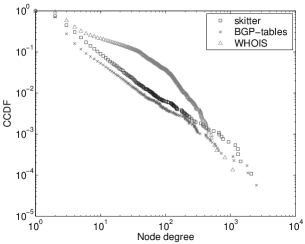
(b) CCDF

(c) PDFs of skitter vs. BGP differences

Figure 1: Node degree distributions $\mathbf{P(k)}$.

Note that there are fewer 1-degree nodes than 2-degree nodes in all the graphs (Figure 1(a)). This effect is due to the AS number assignment policies [15] allowing a customer to have an AS number only if it has multiple providers. If these policies were strictly enforced and if there were no measurement inaccuracies, then the minimum observed AS degree would be 2.

CCDFs of skitter and BGP graphs look similar (Figure 1(b)), but Table 1 shows significant differences between the two graphs in terms of (non-)intersecting nodes and links. We seek to answer the question of where, topologically, these nodes and links are located. Calculating the degree distribution of nodes present only in the BGP graph (Figure 1(c)), we detect a skew toward low-degree nodes. The average degree of the nodes that are present only in BGP graphs, but not in skitter, is $1.86$. skitter’s target list of destinations to probe does not contain IP addresses that respond in the address blocks advertised by these small ASes. As a result, the skitter graph misses them. Most links present only in BGP, but not in skitter, are links between low-degree ASes (see [13] for details). The majority of such links connect the low-degree ASes present only in BGP to their secondary (backup) low-degree providers, while their primary providers are of high degrees. Even if skitter detects a low-degree AS having such a small backup provider, the tool is still unlikely to detect the backup link since its traceroutes follow the primary path via the large provider.

3.3 Joint degree distribution

While the node degree distribution tells us how many nodes of a given degree are in the network, it fails to provide information on the interconnection between these nodes: given $P(k)$, we still do not know anything about the structure of the neighborhood of the average node of a given degree. The joint degree distribution fills this gap by providing information about 1-hop neighborhoods around a node.

Definition. Let $m(k_{1},k_{2})$ be the total number of edges connecting nodes of degrees $k_{1}$ and $k_{2}$. The joint degree distribution (JDD), or the node degree correlation matrix, is the probability that a randomly selected edge connects $k_{1}$- and $k_{2}$-degree nodes: $P(k_{1},k_{2})=\mu(k_{1},k_{2})\times m(k_{1},k_{2})/(2m)$, where $\mu(k_{1},k_{2})$ is $1$ if $k_{1}=k_{2}$ and $2$ otherwise. Note that $P(k_{1},k_{2})$ is different from the conditional probability $P(k_{2}|k_{1})=(\bar{k}P(k_{1},k_{2}))/(k_{1}P(k_{1}))$ that a given $k_{1}$-degree node is connected to a $k_{2}$-degree node. The JDD contains more information about the connectivity in a graph than the degree distribution, since given a specific form of $P(k_{1},k_{2})$ we can always restore both the degree distribution $P(k)$ and average degree $\bar{k}$ by expressions in [9]. A summary statistic of JDD is the the average neighbor connectivity $k_{nn}(k)=\sum_{k^{\prime}=1}^{k_{max}}k^{\prime}P(k^{\prime}|k)$. It is simply the average neighbor degree of the average $k$-degree node. It shows whether ASes of a given degree preferentially connect to high- or low-degree ASes. In a full mesh graph, $k_{nn}(k)$ reaches its maximal possible value, $n-1$. Therefore, for uniform graph comparison we plot normalized values $k_{nn}(k)/(n-1)$. We can further summarize the JDD by a single scalar called assortativity coefficient $r$ [23, 24], $r\sim\sum_{k_{1},k_{2}=1}^{k_{max}}k_{1}k_{2}(P(k_{1},k_{2})-k_{1}k_{2}P(k_{1})P(k_{2})/{\bar{k}}^{2})$.

Importance. The assortativity coefficient $r$, $-1\leq r\leq 1$, has direct practical implications. Disassortative networks with $r<0$ have an excess of radial links, that is, links connecting nodes of dissimilar degrees. Such networks are vulnerable to both random failures and targeted attacks. On a positive note, vertex covers in disassortative graphs are smaller, which is important for applications such as traffic monitoring [25] and prevention of DoS attack [26]. The opposite properties apply to assortative networks with $r>0$ that have an excess of tangential links, that is, links connecting nodes of similar degrees.

In contrast to the widely studied degree distribution, the network community has only recently started recognizing the importance of JDD [30, 7]. In the most prominent recent example [5] Li et al. define likelihood and make this metric central for their argument. They propose to use likelihood, which is directly related to the assortativity coefficient, as a measure of randomness to differentiate between multiple graphs with the same degree distribution. Such a measure is important for evaluating the amount of order, e.g., engineering design constraints, present in a given topology. A topology with low likelihood is not random; it results from some sophisticated evolution processes involving specific design purposes.

Discussion. All the three Internet graphs built from our data sources are disassortative ($r<0$) as seen in Table 2. We call the order of graphs with decreasing assortativity coefficient $r$—WHOIS, BGP, skitter—the $\mathbf{r}$-order.

We can explain the $r$-order in terms of differing topology measurement methodologies. First, we notice that both skitter and BGP graphs are results of tree-like explorations of the network topology, meaning that we can roughly approximate these graphs by a union of spanning trees rooted at, respectively, skitter monitors or BGP data collection points. As such, both these methods are likely to discover more radial links connecting numerous low-degree nodes, i.e., small ASes, to high-degree nodes, i.e., large ISP ASes, where the monitors are located. At the same time, these measurements fail to detect some tangential links interconnecting medium-to-low degree nodes since many of these links belong to none of the spanning trees rooted at the vantage points in the core. In contrast, WHOIS data contains abundant medium-degree tangential links because it relies on operators to report all the links attached to a given AS, i.e., a source of a WHOIS record. This excess of tangential links in WHOIS is thus responsible for its much higher assortativity. Second, we explain that the BGP graph has a slightly higher assortativity than the skitter graph. As discussed in Section 3.2, the BGP graph contains the tangential links between low-degree nodes that traceroute probes of skitter miss since these links are typically the backup links to smaller secondary providers, while skitter’s ICMP packets tend to follow the primary paths to larger primary providers. This small excess of tangential links is responsible for a slightly higher assortativity of the BGP graph compared to skitter.

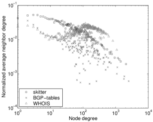
Figure 2: Normalized average neighbor connectivity $\mathbf{k_{nn}(k)/(n-1)}$.

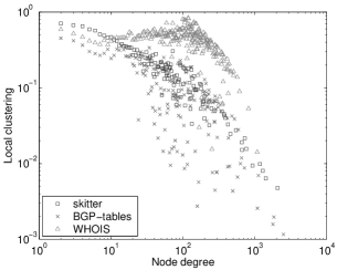
Figure 3: Local clustering $\mathbf{C(k)}$.

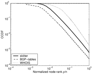
Figure 4: Rich club connectivity $\mathbf{\phi(\rho/n)}$.

The interplay between $\bar{k}$- and $r$-orders underlies Figure 4, where we plot the average neighbor connectivity functions for the three graphs. Skitter has the largest excess of radial links that connect low-degree nodes (customers ASes) to high-degree nodes (large provider ASes). The highest relative number of radial links is responsible for skitter’s highest average degree of the neighbors of low-degree nodes: in Figure 4, skitter is at the top in the area of low degrees, while BGP is below and WHOIS is at the bottom ($r$-order). On the other hand, the greatest proportion of tangential links between ASes of similar degrees in the WHOIS graph contributes to connectivity of neighbors of high-degree nodes; therefore the WHOIS graph is at the top for high-degree nodes ($\bar{k}$-order).

Note that in the case of skitter and BGP, $k_{nn}(k)$ can be approximated by a power law with the corresponding exponents $\gamma_{nn}$ in Table 2.

3.4 Clustering

While JDD contains information about the degrees of neighbors for the average $k$-degree node, it does not tell us how these neighbors interconnect. Clustering partially satisfies this need by providing a measure of how close a node’s neighbors are to forming a clique.

Definition. Let $\bar{m}_{nn}(k)$ be the average number of links between the neighbors of $k$-degree nodes. Local clustering is the ratio of this number to the maximum possible number of such links: $C(k)=\bar{m}_{nn}(k)/{k\choose 2}$. If two neighbors of a node are connected, then these three nodes together form a triangle (3-cycle). Therefore, by definition, local clustering is the average number of 3-cycles involving $k$-degree nodes. The two summary statistics associated with local clustering are mean local clustering $C_{mean}=\sum C(k)P(k)$, which is the average value of $C(k)$, and the clustering coefficient $C_{coeff}$, which is the percentage of 3-cycles among all connected node triplets in the entire graph (for the exact definition, see [31]).

Importance. Clustering expresses local robustness in the graph and thus has practical implications: the higher the local clustering of a node, the more interconnected are its neighbors, thus increasing the path diversity locally around the node. Networks with strong clustering are likely to be chordal or of low chordality, which makes certain routing strategies perform better [32]. One can also use clustering as a litmus test for verifying the accuracy of a topology model or generator [6].

Discussion. We first observe that the clustering average values $C_{mean}$ in Table 2 are in the $\bar{k}$-order, which is expected: clustering increases with increase in number of links. The values of $C_{mean}$ are almost equal for skitter and WHOIS, but the clustering coefficient $C_{coeff}$ is 15 times larger for WHOIS than for skitter. As shown in [33], orders of magnitude difference between $C_{mean}$ and $C_{coeff}$ is intrinsic to highly disassortative networks and is a consequence of strong degree correlations (JDD) necessarily present in such networks.

Similar to $k_{nn}(k)$, the interplay between $\bar{k}$- and $r$-orders explains Figure 4, where we plot local clustering as a function of node degree $C(k)$. Skitter’s clustering is the highest amongst the three graphs for low-degree nodes because this graph is most disassortative. The links adjacent to low-degree nodes are most likely to lead to high-degree nodes, the latter being interconnected with a high probability. The WHOIS graph exhibits the highest values for clustering for high-degree nodes since this graph has the highest average connectivity (largest $\bar{k}$). The neighbors of high-degree nodes are interconnected to a greater extent, resulting in higher clustering for such nodes.

Similar to $k_{nn}(k)$, $C(k)$ also can be approximated by a power law for skitter and BGP graphs (exponents $\gamma_{C}$ in Table 2).

Strong correlations in JDD play a major part for the presence of non-trivial clustering observed in many networks [33]. The interplay between $\bar{k}$- and $r$-orders explains the overall similarity between degree correlations and clustering, in general, and similarity between $k_{nn}(k)$ and $C(k)$, in particular.

3.5 Rich club connectivity

Definition. Let $\rho=1\ldots n$ be the first $\rho$ nodes ordered by their non-increasing degrees in a graph of size $n$. Rich club connectivity (RCC) $\phi(\rho/n)$ is the ratio of the number of links in the subgraph induced by the $\rho$ largest-degree nodes to the maximum possible number of such links $\rho\choose 2$. In other words, the RCC is a measure of how close $\rho$-induced subgraphs are to cliques.

Importance. The Positive Feedback Preference (PFP) model by Zhou and Mondragon [8] has successfully reproduced a wide spectrum of metrics of their measured AS-level topology by trying to explicitly capture only the following three characteristics: (i) the exact form of the node degree distribution; (ii) the maximum node degree; and (iii) RCC. One can show that networks with the same JDDs have the same RCC. The converse is not true, but given a specific form of RCC, one can fully describe all possible JDDs that would yield the specified RCC.

Discussion. As expected, the values of $\phi(\rho/n)$ in Figure 4 are in the $\bar{k}$-order with WHOIS at the top: more links result in denser cliques. RCC exhibits clean power laws for all three graphs in the area of medium and large $\rho/n$. The values of the power-law exponents $\gamma_{rc}$ in Table 2 result from fitting $\phi(\rho/n)$ with power laws for 90% of the nodes, $0.1\leq\rho/n\leq 1$.

3.6 Distance

Definition. The shortest path length distribution or simply the distance distribution $d(x)$ is the probability that a random pair of nodes are at a distance $x$ hops from each other. Two basic summary statistics associated with the distance distribution of a graph are average distance $\bar{d}$ and the standard deviation $\sigma$. We call the latter the distance distribution width since distance distributions in Internet graphs (and in many other networks) have a characteristic Gaussian-like shape.

Figure 5: Distance $\mathbf{d(x)}$ distribution.

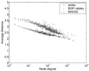
Figure 6: Average distance from $k$-degree nodes $\mathbf{d(k)}$.

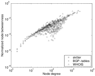
Figure 7: Normalized node betweenness $\mathbf{B(k)/n/(n-1)}$.

Importance. Distance distribution is important for many applications, the most prominent being routing. A distance-based locality-sensitive approach [34] is the root of most modern routing algorithms. As shown in [35], performance parameters of these algorithms depend mostly on the distance distribution. In particular, short average distance and narrow distance distribution width break the efficiency of traditional hierarchical routing. They are among the root causes of interdomain routing scalability issues in the Internet today.

Distance distribution also plays a vital role in robustness of the network to worms. Worms can quickly contaminate a network that has small distances between nodes. Topology models that accurately reproduce observed distance distributions will benefit researchers developing techniques to quarantine the network from worms [36].

We note that expansion, identified in [4] as a critical metric for topology comparison analysis, is a renormalized version of the distance distribution: it is the product of the distance distribution and the graph size $n$.

Discussion. Although the distance distribution is a global topology characteristic, we can explain Figure 7 by the interplay between our local connectivity characteristics: the $\bar{k}$- and $r$-orders. First, we note that the skitter graph stands out in Figure 7 as it has the smallest average distance and the smallest distribution width (Table 2). This result appears unexpected at first since the skitter graph has more nodes than the WHOIS graph and only about half the links. One would expect a denser graph (WHOIS) to have a lower average distance since adding links to a graph can only decrease the average distance in it. Surprisingly, the average distance of the most richly connected (highest $\bar{k}$) WHOIS graph is not the lowest. This result can be explained using the $r$-order. Indeed, a more disassortative graph has a greater proportion of radial links, shortening the distance from the fringe to the core. The skitter graph has the right balance between the relative number of links $\bar{k}$ and their radiality $r$, that minimizes the average distance. Compared to skitter, the BGP graph has larger distance because it is sparser (lower $\bar{k}$), and the WHOIS graph has larger distance because it is more assortative (higher $r$).

Another observation is that for all three graphs, including WHOIS, the average distance as a function of node degree exhibits relatively stable power laws in the full range of node degrees (Figure 7), with exponents given in Table 2.

3.7 Betweenness

Although the average distance is a good node centrality measure—intuitively, nodes with smaller average distances are closer to the graph “center,”—the most commonly used measure of centrality is betweenness. It is applicable not only to nodes, but also to links.

Definition. Betweenness measures the number of shortest paths passing through a node or link and, thus, estimates the potential traffic load on this node/link assuming uniformly distributed traffic following shortest paths. Let $\sigma_{ij}$ be the number of shortest paths between nodes $i$ and $j$ and let $l$ be either a node or link. Let $\sigma_{ij}(l)$ be the number of shortest paths between $i$ and $j$ going through node (or link) $l$. Its betweenness is $B_{l}=\sum_{ij}\sigma_{ij}(l)/\sigma_{ij}$. The maximum possible value for node and link betweenness is $n(n-1)$ [22], therefore in order to compare betweenness in graphs of different sizes, we normalize it by $n(n-1)$.

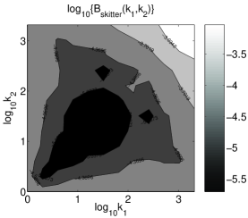
(a) skitter

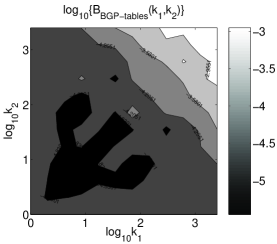
(b) BGP tables

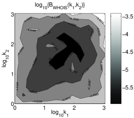
(c) WHOIS

Figure 8: Logarithm of normalized link betweenness $\mathbf{B(k_{1},k_{2})/n/(n-1)}$ on a log-log scale.

Importance. Betweenness is important for traffic engineering applications that try to estimate potential traffic load on nodes/links and potential congestion points in a given topology. Betweenness is also critical for evaluating the accuracy of topology sampling by tree-like probes (e.g. skitter and BGP). As shown in [22], the broader the betweenness distribution, the higher the statistical accuracy of the sampled graph. The exploration process statistically focuses on nodes/links with high betweenness thus providing an accurate sampling of the distribution tail and capturing relevant statistical information. Finally we note that link value, used [4] to analyze the topology hierarchy, and router utilization, used [5] to measure network performance, are both directly related to betweenness.

Discussion. The simplest approach to calculating node betweenness requires long run times, but we used an efficient algorithm from [37]. We had to modify it to also compute link betweenness.

For skitter and BGP graphs, node betweenness is a growing power-law function of node degree (Figure 7) with exponents given in Table 2. An excess of medium degree nodes in the WHOIS graph (Figure 1) leads to greater path diversity and, hence, to lower betweenness values for these nodes.

We also calculate average link betweenness as a function of degrees of nodes adjacent to a link $B(k_{1},k_{2})$ (Figure 8). The contour plots provide information on the betweenness values of the links that connect similar or dissimilar degree nodes. One would expect links connecting high-degree nodes to exhibit highest link betweenness and thereby be used as a measure of link centrality. Contrary to popular belief, the contour plots show that link betweenness does not measure link centrality. First, betweenness of links adjacent to low-degree nodes (the left and bottom sides of the plots) is not the minimum. In fact, non-normalized betweenness of links adjacent to 1-degree nodes is constant and equal to $n-1$ (the number of destinations in the rest of the network). Similar values of betweenness characterize links elsewhere in the graph, including radial links between high and low-to-medium degree nodes and tangential links in the zone of medium-to-high degrees (diagonal zone from bottom-right to upper-left). While the maximum-betweenness links are between high-degree nodes as expected (the upper right corner of the plots), the minimum-betweenness links are tangential in the medium-to-low degree zone (diagonal areas of low values from bottom-left to upper-right). We can explain the latter observation by the following argument. Let $i$ and $j$ be two nodes connected by a minimum-betweenness link $l$. The only shortest paths going through $l$ are those between nodes that are below $i$ and $j$, where “below” means further from the core and closer to the fringe. When the degrees of both $i$ and $j$ are small, the numbers of nodes below them (with lower degree) are small, too. Consequently, the number of shortest paths, proportional to the product of the number of nodes below $i$ and $j$, attains its minimum at $l$. We conclude that link betweenness is not a measure of centrality but a measure of a certain combination of link centrality and radiality.

3.8 Spectrum

Definition. Let $\mathcal{A}$ be the adjacency matrix of a graph. This $n\times n$ matrix is constructed by setting the value of its element $a_{ij}=a_{ji}=1$ if there is a link between nodes $i$ and $j$. All other elements have value $0$. Scalar $\lambda$ and vector $v$ are the eigenvalue and eigenvector respectively of $\mathcal{A}$ if $\mathcal{A}v=\lambda v$. The spectrum of a graph is the set of eigenvalues of its adjacency matrix.

Another closely related and frequently used definition of the graph spectrum is the spectrum of the eigenvalues of its Laplacian, $\mathcal{L}=\mathcal{T}^{-1/2}(\mathcal{T}-\mathcal{A})\mathcal{T}^{-1/2}$, where $\mathcal{T}$ is the diagonal matrix with $t_{ii}$ equal to the degree of node $i$. This definition is a normalized version of the original definition, in the sense that for any graph, all the eigenvalues of its Laplacian are located between $0$ and $2$. We use the original definition in this paper.

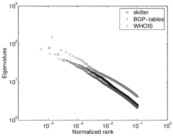
Figure 9: Spectrum. Absolute values of top 10% of eigenvalues ordered by their normalized rank: normalized rank is node rank divided by the total number of nodes in the graph.

Importance. Spectrum is one of the most important global characteristics of the topology. Spectrum yields tight bounds for a wide range of critical graph characteristics [38], such as distance-related parameters, expansion properties, and values related to separator problems estimating graph resilience under node/link removal. The largest eigenvalues are particularly important. Most networks with high values for these largest eigenvalues have small diameter, expand faster, and are more robust.

Two specific examples of spectrum-related metrics that made significant contributions to networking topology research further emphasize the importance of spectrum. First, Tangmunarunkit et al. [4] defined network resilience, one of the three metrics critical for their topology comparison analysis, as a measure of network robustness under link removal, which equals the minimum balanced cut size of a graph. By this definition, resilience is related to spectrum since the graph’s largest eigenvalues provide bounds on network robustness with respect to both link and node removals [38].

Second, Li et al. [5] define network performance, one of the two metrics critical for their HOT argument, as the maximum traffic throughput of the network. By this definition, performance is related to spectrum since it is essentially the network conductance [39] which can be tightly estimated by the gap between the first and second largest eigenvalues [38].

Beyond its significance for network robustness and performance, the graph’s largest eigenvalues are important for traffic engineering purposes since graphs with larger eigenvalues have, in general, more node- and link-disjoint paths to choose from. The spectral analysis of graphs is a powerful tool for detailed investigation of network structure, such as discovering clusters of highly interconnected nodes [40], and possibly revealing the hierarchy of ASes in the Internet [41].

Discussion. Our $\bar{k}$-order (BGP, skitter, WHOIS) plays a key role once again: the densest graph, WHOIS, is at the top in Figure 9 and its first eigenvalue is largest in Table 2. The eigenvalue distributions of all the three graphs follow power laws.

4 Conclusion

We presented a detailed comparison of widely available sources of Internet topology data—skitter, BGP, and WHOIS—in terms of a number of popular metrics studied in the literature. Of the set of metrics we considered, the joint degree distribution (JDD) $P(k_{1},k_{2})$ appears to play a central role in determining a wide range of other topological properties. Indeed, using only the average degree $\bar{k}$ and the assortativity coefficient $r$, the two coarse summary statistics of the JDD, we could explain the relative order of all other metrics for all our data sources. At the same time, we saw that the values of $\bar{k}$ and $r$ are closely connected with the data source properties and collection methodologies. While additional work is required to assess the definitiveness of the JDD in describing topologies, we have demonstrated that it is a powerful metric for capturing a variety of important graph properties. Isolating such an encompassing metric or a small set of metrics is a prerequisite to developing accurate topology generators since it would reduce the number of parameters one has to reproduce. Building a JDD-based topology generator and investigating the roles of degree correlations of higher orders are subjects of our current research.

A number of methods have been proposed [42, 43] to annotate links in AS-level graphs thus incorporating AS relationship information. Although we did not consider AS relationships in this study, we note that the results of our analysis, in general, and JDD-related statistics, in particular, are immediately applicable to directed—or, more generally, annotated—graphs as well.

It remains an open question which data source most closely matches actual Internet AS topology, given that each graph approximates a different view of the Internet looking at the data (skitter), control (BGP), and management (WHOIS) planes. In particular, we want to know what data source contains reliable information about what type of links and how over- or under-reporting of such links affects the metric values in the resulting graphs. This knowledge would allow us to combine information that we trust from all three data sources so that we can obtain the most representative and complete Internet topology view. For now, we see that topologies derived from the three data sources are quantitatively but not qualitatively different: all three degree distributions are scale-free, but not all of them are power laws. We conclude that comparative analysis of these three views allows us to test the limits of metrics’ sensitivity to measurement incompleteness and inaccuracies.

We believe that our work will arm researchers with deeper insights into specifics of each topology view. We hope that this study encourages the validation of existing topology models against real data and motivates the development of better ones.

Table 2: Summary statistics.

		skitter	BGP tables	WHOIS
Average degree	Number of nodes $(n)$	9,204	17,446	7,485
	Number of edges $(m)$	28,959	40,805	56,949
	Avg node degree $(\bar{k})$	6.29	4.68	15.22
Degree distribution	Max node degree $(k_{max})$	2,070	2,498	1,079
	Power-law max degree $(k_{max}^{PL})$	1,448	4,546	-
	Exponent of $P(k)\;(-\gamma)$	2.25	2.16	-
Joint degree distribution	Avg neighbor degree $(\bar{k}_{nn}/(n-1))$	0.05	0.03	0.02
	Exponent of $k_{nn}(k)\;(-\gamma_{nn})$	1.49	1.45	-
	Assortative coefficient $(r)$	-0.24	-0.19	-0.04
Clustering	Mean clustering $(C_{mean})$	0.46	0.29	0.49
	Clustering coefficient $(C_{coeff})$	0.03	0.02	0.31
	Exponent of $C(k)\;(-\gamma_{C})$	0.33	0.34	-
Rich club	Exponent of $\phi(\rho/n)\;(-\gamma_{rc})$	1.48	1.45	1.69
Distance	Avg distance $(\bar{d})$	3.12	3.69	3.54
	Std deviation of distance $(\sigma)$	0.63	0.87	0.80
	Exponent of $d(k)\;(-\gamma_{d})$	0.07	0.07	0.09
Betweenness	Avg node betweenness $(\bar{B}_{node}/(n(n-1)))$	$11\cdot 10^{-5}$	$7.7\cdot 10^{-5}$	$17\cdot 10^{-5}$
	Exponent of $B(k)\;(\gamma_{B})$	1.35	1.17	-
	Avg edge betweenness $(\bar{B}_{edge}/(n(n-1)))$	$5.37\cdot 10^{-5}$	$4.51\cdot 10^{-5}$	$3.10\cdot 10^{-5}$
Spectrum	Largest eigenvalue	79.53	73.06	150.86
	Second largest eigenvalue	-53.32	-55.13	68.63
	Third largest eigenvalue	36.40	53.54	62.03

5 Acknowledgments

We thank Ulrik Brandes for sharing his betweenness code with us, Andre Broido for answering our questions, and anonymous reviewers for their comments that helped to improve this paper.

Support for this work was provided by NSF CNS-0434996, NCS ANI-0221172, Center for Networked Systems (UCSD), and Cisco University Research program.

References

- [1]
- [2] M. Faloutsos, P. Faloutsos, and C. Faloutsos, “On power-law relationships of the Internet topology,” in ACM SIGCOMM, 1999, pp. 251–262.
- [3] Q. Chen, H. Chang, R. Govindan, S. Jamin, S. J. Shenker, and W. Willinger, “The origin of power laws in Internet topologies revisited,” in IEEE INFOCOM, 2002.
- [4] H. Tangmunarunkit, R. Govindan, S. Jamin, S. Shenker, and W. Willinger, “Network topology generators: Degree-based vs. structural,” in ACM SIGCOMM, 2002, pp. 147–159.
- [5] L. Li, D. Alderson, W. Willinger, and J. Doyle, “A first-principles approach to understanding the Internet s router-level topology,” in ACM SIGCOMM, 2004.
- [6] T. Bu and D. Towsley, “On distinguishing between Internet power law topology generators,” in IEEE INFOCOM, 2002.
- [7] S. Jaiswal, A. L. Rosenberg, and D. Towsley, “Comparing the structure of power-law graphs and the Internet AS graph,” in IEEE ICNP, 2004.
- [8] S. Zhou and R. J. Mondragón, “Accurately modeling the Internet topology,” Physical Review E, vol. 70, pp. 066108, 2004, http://arxiv.org/abs/cs.NI/0402011.
- [9] S. N. Dorogovtsev and J. F. F. Mendes, Evolution of Networks: From Biological Nets to the Internet and WWW, Oxford University Press, Oxford, 2003.
- [10] kc claffy, T. E. Monk, and D. McRobb, “Internet tomography,” Nature, January 1999, http://www.caida.org/tools/measurement/skitter/.
- [11] “University of Oregon RouteViews Project,” http://www.routeviews.org/.
- [12] “Internet Routing Registries,” http://www.irr.net/.
- [13] CAIDA, “Comparative analysis of the Internet AS-level topologies extracted from different data sources: Data page,” http://www.caida.org/analysis/topology/as_topo_comparisons/.
- [14] Y. Rekhter and T. Li, A Border Gateway Protocol 4 (BGP-4), IETF, RFC 1771, 1995.
- [15] J. Hawkinson and T. Bates, Guidelines for Creation, Selection, and Registration of an Autonomous System (AS), IETF, RFC 1930, 1996.
- [16] “traceroute,” http://www.traceroute.org/#source%20code.
- [17] CAIDA, “Macroscopic topology AS adjacencies,” http://www.caida.org/tools/measurement/skitter/as_adjacencies.xml.
- [18] Z. M. Mao, J. Rexford, J. Wang, and R. H. Katz, “Towards an accurate AS -level traceroute tool,” in ACM SIGCOMM, 2003.
- [19] G. Siganos and M. Faloutsos, “Analyzing BGP policies: Methodology and tool,” in IEEE INFOCOM, 2004.
- [20] H. Chang, R. Govindan, S. Jamin, S. J. Shenker, and W. Willinger, “Towards capturing representative AS-level Internet topologies,” Computer Networks Journal, vol. 44, pp. 737–755, April 2004.
- [21] A. Lakhina, J. Byers, M. Crovella, and P. Xie, “Sampling biases in IP topology measurements,” in IEEE INFOCOM, 2003.
- [22] L. Dall’Asta, I. Alvarez-Hamelin, A. Barrat, A. Vázquez, and A. Vespignani, “Exploring networks with traceroute-like probes: Theory and simulations,” Theoretical Computer Science, Special Issue on Complex Networks, 2005, http://arxiv.org/abs/cs.NI/0412007.
- [23] M. E. J. Newman, “Assortative mixing in networks,” Physical Review Letters, vol. 89, no. 20, pp. 208701, 2002.
- [24] S. N. Dorogovtsev, “Networks with given correlations,” http://arxiv.org/abs/cond-mat/0308336v1.
- [25] Y. Breitbart, C.-Y. Chan, M. Garofalakis, R. Rastogi, and A. Silberschatz, “Efficiently monitoring bandwidth and latency in IP networks,” in IEEE INFOCOM, 2001.
- [26] K. Park and H. Lee, “On the effectiveness of route-based packet filtering for distributed DoS attack prevention in power-law internets,” in ACM SIGCOMM, 2001.
- [27] CAIDA, “Visualizing Internet topology at a macroscopic scale,” http://www.caida.org/analysis/topology/as_core_network/.
- [28] I. Alvarez-Hamelin, L. Dall’Asta, A. Barrat, and A. Vespignani, “-core decomposition: A tool for the visualization of large scale networks,” http://arxiv.org/abs/cs.NI/0504107.
- [29] S. Tauro, C. Palmer, G. Siganos, and M. Faloutsos, “A simple conceptual model for the Internet topology,” in Global Internet, 2001.
- [30] J. Winick and S. Jamin, “Inet-3.0: Internet topology generator,” Technical Report UM-CSE-TR-456-02, University of Michigan, 2002.
- [31] B. Bollobás and O. Riordan, “Mathematical results on scale-free random graphs,” in Handbook of Graphs and Networks, Berlin, 2002, Wiley-VCH.
- [32] P. Fraigniaud, “A new perspective on the small-world phenomenon: Greedy routing in tree-decomposed graphs,” in ESA, 2005.
- [33] S. N. Soffer and A. Vázquez, “Clustering coefficient without degree correlations biases,” http://arxiv.org/abs/cond-mat/0409686.
- [34] D. Peleg, Distributed Computing: A Locality-Sensitive Approach, SIAM, Philadelphia, PA, 2000.
- [35] D. Krioukov, K. Fall, and X. Yang, “Compact routing on Internet-like graphs,” in IEEE INFOCOM, 2004.
- [36] C. Shannon and D. Moore, “The spread of the witty worm,” in Proceedings of IEEE Security and Privacy, July 2004.
- [37] U. Brandes, “A faster algorithm for betweenness centrality,” Journal of Mathematical Sociology, vol. 25, no. 2, pp. 163–177, 2001.
- [38] F. K. R. Chung, Spectral Graph Theory, vol. 92 of Regional Conference Series in Mathematics, American Mathematical Society, Providence, RI, 1997.
- [39] C. Gkantsidis, M. Mihail, and A. Saberi, “Conductance and congestion in power law graphs,” in ACM SIGMETRICS, 2003.
- [40] D. Vukadinović, P. Huang, and T. Erlebach, “A spectral analysis of the Internet topology,” Technical Report TIK-NR. 118, ETH, 2001.
- [41] C. Gkantsidis, M. Mihail, and E. Zegura, “Spectral analysis of Internet topologies,” in IEEE INFOCOM, 2003.
- [42] L. Subramanian, S. Agarwal, J. Rexford, and R. H. Katz, “Characterizing the Internet hierarchy from multiple vantage points,” in IEEE INFOCOM, 2002.
- [43] X. Dimitropoulos, D. Krioukov, B. Huffaker, kc claffy, and G. Riley, “Inferring AS relationships: Dead end or lively beginning?,” in WEA, 2005.