Fundamental Limits and Scaling Behavior of Cooperative Multicasting in Wireless Networks

Abstract

A framework is developed for analyzing capacity gains from user cooperation in slow fading wireless networks when the number of nodes (network size) is large. The framework is illustrated for the case of a simple multipath-rich Rayleigh fading channel model. Both unicasting (one source and one destination) and multicasting (one source and several destinations) scenarios are considered. We introduce a meaningful notion of Shannon capacity for such systems, evaluate this capacity as a function of signal-to-noise ratio (SNR), and develop a simple two-phase cooperative network protocol that achieves it. We observe that the resulting capacity is the same for both unicasting and multicasting, but show that the network size required to achieve any target error probability is smaller for unicasting than for multicasting. Finally, we introduce the notion of a network “scaling exponent” to quantify the rate of decay of error probability with network size as a function of the targeted fraction of the capacity. This exponent provides additional insights to system designers by enabling a finer grain comparison of candidate cooperative transmission protocols in even moderately sized networks.

I Introduction

Cooperative diversity has been proposed as an attractive approach to combatting slow fading in wireless networks [13, 8]. Spatially distributed nodes provide an opportunity to create a distributed virtual antenna array and can provide substantial gains in slow fading environments. There has been a significant interest in studying these gains recently; see, e.g., [9, 1, 10, 12, 2] and the references therein.

A convenient channel model for such problems, as has been widely adopted in the literature, is a quasistatic one in which the parameters are known to receivers, but not to transmitters. In such scenarios the classical Shannon capacity is typically zero due to the positive probability of the channel experiencing an arbitrarily deep fade, so performance is instead quantified in terms of outage capacity, which describes the achievable rate subject to a constraint on the level of outage probability that can be tolerated [11].

Outage analysis applies to a host of multiterminal extensions of such basic channel models as well [14], although the expressions become more cumbersome. To address this, diversity-multiplexing tradeoff analysis provides a suitably coarser scale characterization of such systems by focusing on the high signal-to-noise ratio (SNR) regime and examining how outage probability scales with SNR in this regime for different transmission rates [16].

Diversity-multiplexing tradeoff analysis has also proven useful analyzing a host of simple network problems. For example, [15] extends the analysis to the multiple-access channel, while [8] extends the analysis to the cooperative diversity channel.

While such analysis of cooperative diversity has proven popular, much of the work has been limited to systems in which for a given message there is effectively only a single destination node and a relatively small number of potential relay nodes to participate in the transmission.

In the present paper, we develop an alternative framework within which to examine cooperative protocols. First, our emphasis is on the multicasting scenario in which there is one message in the network, but generally multiple destination nodes. We will focus on two extreme special cases of this scenario. One is when all nodes in the network are to receive the message, which for convenience we generically refer to as multicasting. The other is when exactly one node in the network is to receive the message, which we refer to as unicasting.

Second, our framework examines the scenario in which the number of nodes in the network is large. This will allow us to examine the associated asymptotic scaling behavior of cooperative networks. As a by-product, we do not need to restrict our attention to high SNR analysis. Indeed, we fix the noise power, normalize the channel statistics, and contrain the total power transmitted in the network. This allows us to parameterize our results in terms of the associated SNR.

Within this framework, we analyze the relationship between transmission rate and the associated error probability. Provided we use codes of sufficiently long block lengths, outage probability dominates the error probability. Specifically, the associated outage event is that not all the intended recipients are able to decode the message. Not suprisingly, avoiding outage in multicasting is more difficult than in unicasting.

As our main result, we show that under a multipath-rich Rayleigh fading network model, a notion of Shannon capacity can be developed. Specifically, there exists a nonzero capacity (dependent on SNR) such that for all rates below capacity, the error probability can be made arbitrarily small provided the network is sufficiently large. Conversely, for all rates above capacity, the error probability is bounded away from zero regardless of network size. Our achievability result is based on a simple two-phase cooperative network protocol we develop. By contrast, when one precludes the possibility of cooperation, the associated capacity is of course zero. Interestingly, our analysis also reveals that despite the fact that multicasting outage behavior is dominated by the worst node, the multicasting and unicasting capacities thus defined are identical. Not surprisingly, we also show that for a fixed number of nodes, the probability of error is still much smaller in unicasting than in multicasting.

We further show that finer scale characterizations of behavior are possible too. In particular, we define a notion of network scaling exponent that characterizes the rate of decay of error probability with network size as a function of the targeted fraction of capacity. Within this analysis, we see, among other insights, that the exponent of our capacity-achieving protocol is quite small for rates that exceed half the network capacity.

While our results are specific to our multipath-rich Rayleigh fading model, we believe that the associated framework is useful more broadly in the analysis of user cooperation gains in large networks with more realistic — if more complicated — models. Indeed, ultimately our results more generally suggest that just as system analysis asymptotic in block length or SNR has proven useful, so can one that is asymptotic in network size.

The remainder of the paper is organized as follows. Section II introduces the network model of interest. The capacity result is stated in Section III. It is established by providing a converse in Section IV and an achievability argument in Section V. The scaling of the outage probability with the number of nodes is discussed in Section VI, and the network scaling exponent is introduced in Section VII. Finally, Section VIII contains some concluding remarks and directions for future work.

II System Model

We consider a system with $K$ receiving nodes and one source node. For convenience, we label the source node as node 0, and the receiving nodes as $\{1,2,\dots,K\}$. Of course, in practice, different nodes in the network can act as source nodes over orthogonal time or frequency bands as discussed in [8]. However, for analysis, it suffices to focus on a single configuration.

We assume a narrowband, slow fading channel passband channel model corresponding to a multipath-rich propagation environment. In particular, the channel gains $h_{jk}$ between arbitrary distinct pairs of nodes $(j,k)$ are independent identically distributed (i.i.d.) random variables from a zero-mean, unit-variance circularly symmetric complex Gaussian distribution. In turn, the signal received at node $k$ at time $i$ is given by

$$y_{k}(i)=\sum_{j\in{\mathcal{T}}(i)}h_{jk}\,x_{j}(i),+z_{k}(i),$$ (1)

where ${\mathcal{T}}(i)$ is the set of nodes transmitting at time $i$, where $x_{j}(i)$ is the symbol transmitted by node $j$ at time $i$, and where $z_{k}(i)$ denotes circularly symmetric complex i.i.d. Gaussian noise of power $N_{0}$. Furthermore, the noises among the different receivers are mutually independent.

In our model, nodes are subject to a half-duplex constraint, i.e., a node cannot transmit and receive simultaneously. Thus, associated with every valid protocol is a set of binary variables of the form $D_{k}(i)$ that specifies at time $i$ whether node $k$ is transmitting ($D_{k}(i)=1$) or receiving ($D_{k}(i)=0$).

The source sends one of $M$ possible messages to the destination node(s) over $n$ channel uses (i.e, $i=1,2,\dots,n$). The channel gains between all pairs of nodes remains fixed over this duration. In our model, the channel gain $h_{jk}$ is known to the receiving node $k$ but not to the transmitting node $j$.

We further restrict our attention to protocols in which relay nodes cannot revert to receive mode once they begin transmitting, i.e., if $D_{k}(i)=1$ for some node $k$ and $i<n$ then $D_{k}(j)=1$ for all $i\leq j\leq n$. This restriction precludes protocols in which transmitting nodes effectively learn and exploit the network channel gains in their encodings.

Finally, for simplicity, we adopt a long-term sum power constraint across the nodes in our model. In particular, with $X_{j}(i)$ for $j\in{\mathcal{T}}(i)$ denoting the (complex-valued) symbol being transmitted by node $j$ at time $i$, we impose an expected sum power constraint of the form

$$E\left[\frac{1}{n}\sum_{i=1}^{n}\sum_{k\in{\mathcal{T}}(i)}|X_{k}(i)|^{2}\right]\leq P,$$ (2)

where the expectation is taken over the ensemble of channel realizations and the set ${\mathcal{T}}(i)$, as well as any other randomized aspects of the protocol. Indeed, one will want to consider protocols in which the set ${\mathcal{T}}(i)$ depends on the realized channel gains.

The power constraint (2) is a rather natural one for systems in which there are ergodic channel variations but a stringent delay constraint that requires transmission of any particular message within a single coherence interval. Indeed, although we do not satisfy the sum power constraint during the transmission of an individual message, the expectation in (2) ensures that it will be satisfied with high probability over a sufficiently long sequence of messages. Nevertheless, we remark in advance that the results of the paper do not change when the we require the sum power constraint to be met with high probability in every coherence interval, and our capacity-achieving protocol can be readily extended to this case. Ultimately, the expected power constraint merely simplifies the exposition.

The preceding discussion characterizes an admissible protocol for our analysis, which we formalize in the following definition.

Definition 1

An admissible protocol $\pi_{K}$ consists of a set of indicator functions $\{D_{k}(i)\}\in\{0,1\}$, which determines whether node $k$ is transmitting or receiving at time $i$; a set of encoding functions $\{\phi_{k}(i)\}\in\mathbb{C}$, which determines the symbol produced by node $k$ at time $i$; and a set of decoding functions $\{\psi_{k}\}\in\{1,2,\dots,M\}$, which determines the message decisions produced by node $k$ at time $n$. These functions are further constrained by their usage as described below.

During the initialization phase of the protocol, the source node 0 selects message $W\in\{1,2,\dots,M\}$ for transmission. The protocol chooses a priori the sequence $D_{0}(i)$ for $i=1,2,\dots,n$. Without loss of generality, $D_{0}(1)=1$ and $D_{k}(1)=0$ for $k=1,2,\dots,K$. Moreover, the collections of observations ${\mathcal{Y}}_{k}$ at each node $k$ are initialized: ${\mathcal{Y}}_{k}=\emptyset$.

At time $i$, for $1\leq i<n$, if $D_{0}(i)=1$, then source node 0 uses encoding function $\phi_{0}(i)$ to map $W$ into a transmitted complex-valued symbol $x_{0}(i)$.

If node $k\in\{1,2,\dots,K\}$ is in transmit mode at that time (i.e., $D_{k}(i)=1$), the encoding function $\phi_{k}(i)$ at node $k$ maps ${\mathcal{Y}}_{k}$ and the complex-valued channel gains $\{h_{jk},j=0,1,\dots,K\}$ into a transmitted complex-valued symbol $x_{k}(i)$, which is transmitted over the channel.

If, instead, the node is in receive mode (i.e., $D_{k}(i)=0$), then it collects the complex-valued measurement $y_{k}(i)$ and updates its set of received symbols via ${\mathcal{Y}}_{k}:={\mathcal{Y}}_{k}\cup\{y_{k}(i)\}$. If $i=n$, the decoding function $\psi_{k}$ at node $k$ maps ${\mathcal{Y}}_{k}$ and the complex-valued channel gains $\{h_{jk},j=0,1,\dots,K\}$ into a decision $\hat{W}_{k}$. Note that without loss of generality, $D_{k}(n)=0$ for at least one value of $k$. If $i<n$, the node makes a decision whether to switch to transmit mode for the remaining duration. If it decides to switch, it sets $D_{k}(j)=1$ for $i+1\leq j\leq n$; otherwise, it sets $D_{k}(i+1)=0$.

A cooperation-free protocol is a special case of the above definition:

Definition 2

A cooperation-free admissible protocol is one for which only the source node transmits, i.e., $D_{k}(i)=0$ for $1\leq k\leq K$ and $1\leq i\leq n$.

III Coding Theorems

We now develop the relationship between transmission rate and error probability for such protocols, in the limit of large network sizes.

We begin with a meaningful definition of capacity.

Definition 3

A rate $R$ is achievable for the unicasting (respectively, multicasting) system if for every network size $K$, there exists an admissible protocol $\pi_{K}$ with $n_{K}$ channel uses and $M_{K}=2^{n_{K}R}$ messages such that the probability that the destination node (respectively, any node) fails to decode the message approaches zero as $K\rightarrow\infty$. The (unicasting or multicasting) capacity $C$ is the supremum of all achievable rates.

With this definition, we have the following coding theorem, which is our main result.

Theorem 1

The unicasting and multicasting capacities are identical and given by

$$C=\log\left(1+\frac{P}{N_{0}}\right),$$ (3)

where $P$ is as defined in (2) and $N_{0}$ is the noise power as defined via (1).

Before presenting our proof of this result, we note that to achieve capacity — indeed any nonzero rate — requires the use of cooperation. Formally, we have the following result.

Theorem 2

The capacity of cooperation-free admissible protocols for both unicasting and multicasting is

$$C_{\mathrm{nc}}=0$$ (4)

whenever $P$ in (2) is finite and $N_{0}$ in (1) is nonzero.

Proof:

From Definition 2, a destination node must decode directly from the source transmission. Since the channel is a Rayleigh fading channel with $P/N_{0}<\infty$, there exists a strictly positive probability of outage — and hence probability of error — for every positive transmission rate $R$. Since these probabilities are independent of $K$, (4) follows. ∎

We now proceed to the proof of Theorem 1. Since we consider large block lengths, error probability is dominated by outage probability. Specifically, we consider blocks long enough that the probability of error when there is no outage is negligible compared to the outage probability. Thus, in the error analysis in our proof, we restrict our attention to outage probability.

IV Proof of Converse Part

We develop a converse via a simple upper bound on the achievable rate $R$ of Definition 3. In particular, suppose a genie conveys the message $W$ to nodes $1,2,\dots,K-1$ and only destination node $K$ remains to be served. Thus, nodes $0,1,\dots,K-1$ can coordinate to send the message to destination node $K$. This is clearly a multiple-input single-output (MISO) antenna system with $K$ antenna elements and channel knowledge only at the receiver. Thus, for a given rate $R$, a lower bound on the outage probability for the MISO channel is a lower bound on that for both unicasting and multicasting systems. We let ${\mathcal{E}}_{K}^{\mathrm{MISO}}$ denote the MISO channel outage event.

To develop such a bound, we first note that it suffices to restrict the input distribution to Gaussian.

Lemma 1 (Teletar [14])

The outage capacity of the slow-fading MISO channel with $K$ transmit antennas in i.i.d. Rayleigh fading with total power constraint $P$ is achieved by an input distribution with a covariance matrix $\operatorname{diag}(P_{1},P_{2},\dots,P_{K})$, where $\sum_{j=1}^{K}P_{j}=P$.

We now establish the following lemma:

Lemma 2

Let $\epsilon>0$ be arbitrary, and let

$$R=\log\left(1+\frac{P}{N_{0}}\right)+\epsilon$$

for a $K$-antenna MISO channel. Then the outage probability $\Pr\{{\mathcal{E}}_{K}^{\mathrm{MISO}}\}$ is bounded away from zero, i.e.,

$$\inf_{K}\Pr\{{\mathcal{E}}_{K}^{\mathrm{MISO}}\}>0.$$ (5)

Proof:

Let $P^{*}_{1},P^{*}_{2},\ldots P^{*}_{K}$ be the power allocations that minimize the outage event for the selected rate. The corresponding mutual information is given by

$$I=\log\left(1+\frac{1}{N_{0}}\sum_{i=1}^{K}P^{*}_{i}|h_{iK}|^{2}\right)$$ (6)

The outage event ${\mathcal{E}}_{K}^{\mathrm{MISO}}=\left\{R>I\right\}$ is bounded as follows:

$$\Pr\{{\mathcal{E}}_{K}^{\mathrm{MISO}}\} =1-\Pr(I\geq R)$$

$$\geq 1-\frac{E\left\{\log\left(1+\frac{1}{N_{0}}\sum_{i=1}^{K}P^{*}_{i}|h_{iK}|^{2}\right)\right\}}{R}$$ (7)

$$\geq 1-\frac{\log\left(1+\frac{1}{N_{0}}\sum_{i=1}^{K}E[|h_{iK}|^{2}]P^{*}_{i}\right)}{R}$$ (8)

$$=1-\frac{\log\left(1+\frac{1}{N_{0}}\sum_{i=1}^{K}P^{*}_{i}\right)}{R}$$ (9)

$$=1-\frac{\log\left(1+\frac{P}{N_{0}}\right)}{R}=\frac{\varepsilon}{R}>0.$$

In the above derivation (7) follows from the Markov inequality, (8) is a consequence of Jensen’s inequality and (9) follows from the Rayleigh model $E[|h_{iK}|^{2}]=1,\forall i$. Since the above result holds for all $K$, (5) follows.

∎

V Proof of Forward Part

A simple two-phase cooperative protocol can achieve any rate below the capacity (3), as we now develop.

V-A A Two-Phase Cooperative Protocol

The protocol of interest is depicted in Fig. 1. Specifically, in phase 1, the source node broadcasts the message over $n_{1}$ channel uses at a rate $R_{1}$ and all nodes attempt to decode the message. Then, in phase 2, the nodes that are successful in decoding the message act as relays and form a virtual antenna array, transmitting over the remaining $n_{2}=n-n_{1}$ channel uses at a rate $R_{2}$. At this point the intended destination(s) attempt(s) to decode the message and an outage is declared if any of the intended destinations fail.

Figure 1: The two-phase cooperative multicasting protocol. In phase 1 (left), the source node (square) broadcasts at a high rate and only a small fraction (solid) of the many destination nodes (discs) are able to decode. In phase 2 (right), these nodes cooperatively broadcast the message to the remaining nodes using a suitable space-time code.

Codebook Generation

Suppose that the source generates $M$ codewords i.i.d. ${\mathcal{CN}}(0,P_{1})$ for some $P_{1}>0$, each of length $n_{1}$, and all other nodes each generate $M$ codewords i.i.d. ${\mathcal{CN}}(0,P_{2})$ for some $P_{2}>0$, each of length $n_{2}$. We describe the main steps of the protocol for the case of multicasting, but indicate the straightforward modifications for the case of unicasting.

Phase 1

The source transmits the codeword corresponding to the intended message from its codebook over $n_{1}$ channel uses. We choose the rate in this phase to be (strictly less than, but arbitrarily close to)

$$R_{1}(\alpha)=\log_{2}\left(1+G(\alpha)\frac{P}{N_{0}}\right),$$ (10)

where

$$G(\alpha)=F^{-1}(1-\alpha),$$ (11)

and $F(\cdot)$ denotes the cumulative distribution function of an arbitrary channel gain $|h_{ij}|^{2}$, and where we have made the dependency of $R_{1}$ on $\alpha$ explicit.

All nodes attempt to decode the transmission. A node is successful in decoding the message if it finds a codeword in the source codebook that is jointly typical with the received sequence. Let $K_{1}$ be the number of nodes that are successful in decoding the message from the source. We label these nodes as $1,2,\dots,K_{1}$. These nodes participate in phase 2.

Phase 2

Each of the $K_{1}$ nodes successful in decoding the phase 1 transmission next transmits the corresponding codeword from its codebook over $n_{2}$ channel uses. The rate in this phase is set to (strictly less than, but arbitrarily close to)

$$R_{2}(\beta)=\log\left(1+\frac{P}{N_{0}}(1-\beta)\right),$$ (12)

where $0<\beta<1$ is design parameter, the dependence of $R_{2}$ on which we have made explicit.

Each of the remaining $K_{2}=K-K_{1}$ nodes attempts to decode the message at the end of the second phase. Node $k$, upon receiving is observations $y_{k}^{n_{2}}$ finds a message $\hat{w}_{k}$ and a subset of nodes ${\mathcal{S}}_{k}=\{k_{1},k_{2},\dots,k_{|{\mathcal{S}}_{k}|}\}\subseteq\{1,2,\dots,K\}\setminus\{k\}$ such that the corresponding set of codewords $\{x_{k_{1}}^{n_{2}}(\hat{w}_{k}),x_{k_{2}}^{n_{2}}(\hat{w}_{k}),\dots,x_{k_{|{\mathcal{S}}_{k}|}}^{n_{2}}(\hat{w}_{k})\}$ is jointly typical with $y_{k}^{n_{2}}$. It declares the message $\hat{w}_{k}$ to be the transmitted message if a unique pair $(\hat{w}_{k},{\mathcal{S}}_{k})$ exists and declares a failure otherwise.

In the case of unicasting, if the destination node is successful in decoding the message in phase 1 then it does not participate in phase 2. Otherwise it continues to listen to the transmissions and attempts to decode the phase 2 transmission. An error occurs if the destination fails to decode the phase 2 transmission.

V-B Protocol Analysis

First, we analyze code rate. To begin, it is straightforward to verify that $n_{1}$ and $n_{2}$ are completely determined by the choice of rates. In particular, let the overall rate of our protocol be $R$, so that there are $M=2^{nR}$ possible messages to send over $n$ channel uses in the system. Then it follows that

$$n_{1}R_{1}=n_{2}R_{2}=\log M.$$ (13)

From (13) it is straightforward to calculate the overall effective rate $R$ of the system. In particular, since $\log M=nR$ and since $n_{1}+n_{2}=n$, (13) implies that $R$ satisfies

$$\frac{1}{R}=\frac{1}{R_{1}(\alpha)}+\frac{1}{R_{2}(\beta)}.$$ (14)

Second, we analyze the power constraint (2). In phase 1, the transmitted power is $P_{1}$, so provided $P_{1}\leq P$, our power constraint is met in this phase. To analyze the power used in phase 2, we begin by noting that on average a fraction $\alpha$ of the nodes are able to decode the message after phase 1. Specifically, the number of nodes $K_{1}$ successful in phase 1 has mean

$$E[K_{1}]=\alpha K$$ (15)

since $K_{1}$ is a binomial random variable, viz., (cf. (10))

$$K_{1}=\sum_{i=1}^{K}1_{\{|h_{0i}|^{2}>G(\alpha)\}},$$ (16)

where $1_{\{\cdot\}}$ is an indicator function, which equals 1 if its subscript is true and 0 otherwise, and where we have set $P_{1}=P$. Hence,

$$E\left[\sum_{j=1}^{K_{1}}|X_{j}|^{2}\right]=P_{2}E[K_{1}]=P_{2}\alpha K,$$

from which we see that the power constraint is satisfied in phase 2 provided $P_{2}\leq P/\alpha K$.

Finally, we analyze the outage probility, i.e., the probability of outage of a node that is unable to decode at the end of the protocol. For convenience, let us exploit symmetry and label this node $K$, while the nodes that are successful in phase 1 we label $1,2,\dots K_{1}$. From straightforward MISO system analysis, node $K$ will fail to decode the message whenever $K_{1}<K$ and

$$R_{2}(\beta)\geq\log\left(1+G_{K}(K_{1})\frac{P}{N_{0}}\right),$$ (17)

where

$$G_{k}(k_{1})\stackrel{{\scriptstyle\Delta}}{{=}}\frac{1}{\alpha K}\sum_{j=1}^{k_{1}}|h_{jk}|^{2}$$ (18)

is the effective MISO channel gain of node $k$, and where we have set $P_{2}=P/(\alpha K)$. But since $R_{2}$ was chosen according to (12) in phase 2, (17) implies that outage will occur when $G_{K}(K_{1})\leq 1-\beta$. Accordingly, the outage events ${\mathcal{E}}^{\mathrm{uc}}_{\alpha,\beta,K}$ and ${\mathcal{E}}^{\mathrm{mc}}_{\alpha,\beta,K}$ for unicasting and multicasting, respectively, take the form

$${\mathcal{E}}^{\mathrm{uc}}_{\alpha,\beta,K} =\bigcup_{k_{1}=0}^{K-1}{\mathcal{A}}_{k_{1}}^{\mathrm{uc}}$$

$${\mathcal{E}}^{\mathrm{mc}}_{\alpha,\beta,K} =\bigcup_{k_{1}=0}^{K-1}{\mathcal{A}}_{k_{1}}^{\mathrm{mc}}$$

where, for $k_{1}\in\{1,2,\dots,K\}$,

$${\mathcal{A}}_{k_{1}}^{\mathrm{uc}} =\left\{K_{1}=k_{1},\quad G_{K}(k_{1})\leq 1-\beta\right\}$$

$${\mathcal{A}}_{k_{1}}^{\mathrm{mc}} =\left\{K_{1}=k_{1},\quad\min_{k:k_{1}\leq k\leq K}G_{k}(k_{1})\leq 1-\beta\right\}$$

The following lemma provides bound on the conditional outage probability that will be useful in the sequel.

Lemma 3

Suppose $k_{1}\geq\alpha K(1-\beta)$ nodes are successful at the end of phase 1. Then the conditional probability of outage is given by

$$\Pr\{{\mathcal{E}}^{\mathrm{uc}}_{\alpha,\beta,K}\mid K_{1}=k_{1}\}\leq\left(\frac{\alpha K(1-\beta)e}{k_{1}}\right)^{k_{1}}e^{-\alpha K(1-\beta)}.$$ (19)

Proof:

To obtain (19), it suffices to bound $\Pr\{G_{K}(K_{1})\leq 1-\beta\mid K_{1}=k_{1}\}$ since $\Pr\{{\mathcal{E}}^{\mathrm{uc}}_{\alpha,\beta,K}\mid K_{1}=k_{1}\}=\Pr\{G_{K}(K_{1})\leq 1-\beta\mid K_{1}=k_{1}\}$. This can be accomplished by the Chernoff bound, since $G_{K}(k_{1})$ in (18) can be written as

$$G_{K}(k_{1})=\sum_{j=1}^{k_{1}}g_{j}$$ (20)

where the

$$g_{j}=\frac{1}{\alpha K}|h_{jK}|^{2}.$$ (21)

are i.i.d. random variables. Specifically, we obtain, for any $s>0$,

$$\Pr\{G_{K}(K_{1})\leq 1-\beta\mid K_{1}=k_{1}\}$$ (22)

$$=\Pr\left\{e^{-sG_{K}(K_{1})}\geq e^{-s(1-\beta)}\biggm{|}K_{1}=k_{1}\right\}$$ (23)

$$\leq e^{s(1-\beta)}E\left[e^{-sG_{K}(K_{1})}\mid K_{1}=k_{1}\right]$$ (24)

$$=e^{s(1-\beta)}\left(E[e^{-sg_{i}}]\right)^{k_{1}}$$ (25)

$$=\frac{e^{s(1-\beta)}}{\left(1+s/(\alpha K)\right)^{k_{1}}},$$ (26)

where (24) follows from the Markov inequality, (25) follows by from (20), and (26) follows from evaluating the characteristic function of the exponential random variables (21).

In turn, since (26) holds for all $s>0$, we can choose the particular value

$$s=\frac{k_{1}}{1-\beta}-\alpha K.$$ (27)

Substituting (27) into (26) yields (19) as desired. ∎

We now show that the probability of outage can be made arbitrarily small by selecting $\alpha K$ appropriately.

Proposition 1

The probability of outage in unicasting decreases exponentially with $\alpha K$ for every $\beta>0$. Specifically, for every $0<\epsilon<\beta$,

$$\Pr\{{\mathcal{E}}^{\mathrm{uc}}_{\alpha,\beta,K}\} =E\left[\Pr\{{\mathcal{E}}^{\mathrm{uc}}_{\alpha,\beta,K}|K_{1}\}\right]$$ (28)

$$\leq\exp(-\alpha K\epsilon^{2}/4)+\exp\left\{\alpha K\gamma(\beta,\epsilon)\right\},$$

where

$$\gamma(\beta,\epsilon)\stackrel{{\scriptstyle\Delta}}{{=}}\beta-\epsilon+(1-\epsilon)\ln\left(\frac{1-\beta}{1-\epsilon}\right)<0.$$ (29)

Proof:

To obtain (28) we observe that, for some $\epsilon\in(0,\beta)$,

$$\Pr\{{\mathcal{E}}^{\mathrm{uc}}_{\alpha,\beta,K}\}$$

$$=\sum_{k_{1}:k_{1}<\alpha K(1-\epsilon)}\Pr\{{\mathcal{E}}^{\mathrm{uc}}_{\alpha,\beta,K}\mid K_{1}=k_{1}\}\Pr\{K_{1}=k_{1}\}$$

$$\quad+\quad\sum_{k_{1}:k_{1}\geq\alpha K(1-\epsilon)}\Pr\{{\mathcal{E}}^{\mathrm{uc}}_{\alpha,\beta,K}\mid K_{1}=k_{1}\}\Pr\{K_{1}=k_{1}\}$$ (30)

$$\leq\Pr\{K_{1}<\alpha K(1-\epsilon)\}+\max_{\stackrel{{\scriptstyle k_{1}:}}{{k_{1}\geq\alpha K(1-\epsilon)}}}\Pr\{{\mathcal{E}}^{\mathrm{uc}}_{\alpha,\beta,K}\mid K_{1}=k_{1}\}$$

$$=\Pr\{K_{1}<\alpha K(1-\epsilon)\}+\Pr\{{\mathcal{E}}^{\mathrm{uc}}_{\alpha,\beta,K}\mid K_{1}=\alpha K(1-\epsilon)\},$$ (31)

where (31) exploits that outage probability is a decreasing function of $k_{1}$. Finally, using the binomial Chernoff bound (see, e.g., [4])

$$\Pr\{K_{1}<\alpha K(1-\epsilon)\}\leq e^{-\alpha K\epsilon^{2}/4},$$

for the first term in (31), and applying Lemma 3 to the second term, yields (28) as desired. ∎

In turn, Proposition 1 can be used to bound the corresponding probability of outage in multicasting.

Proposition 2

The probability of outage in multicasting decays asymptotically with $\alpha K$. Specifically,

$$\Pr\{{\mathcal{E}}^{\mathrm{mc}}_{\alpha,\beta,K}\}=E\left[\Pr\{{\mathcal{E}}^{\mathrm{mc}}_{\alpha,\beta,K}|K_{1}\}\right]\leq K\Pr\{{\mathcal{E}}^{\mathrm{uc}}_{\alpha,\beta,K}\}.$$ (32)

Proof:

First, we bound the conditional outage probability according to

$$\Pr\{{\mathcal{E}}^{\mathrm{mc}}_{\alpha,\beta,K}|K_{1}=k_{1}\}$$ (33)

$$=\Pr\{\min_{k:k_{1}\leq k\leq K}G_{k}(K_{1})<1-\beta|K_{1}=k_{1}\}$$

$$=\Pr\left\{\bigcup_{i=K_{1}+1}^{K}\left\{G_{i}(K_{1})\leq 1-\beta\right\}\Biggm{|}K_{1}=k_{1}\right\}$$

$$\leq(K-k_{1})\Pr\{{\mathcal{E}}^{\mathrm{uc}}_{\alpha,\beta,K}|K_{1}=k_{1}\}$$ (34)

$$\leq K\Pr\{{\mathcal{E}}^{\mathrm{uc}}_{\alpha,\beta,K}|K_{1}=k_{1}\}.$$ (35)

where (34) is a simple application of the union bound. Taking the expectation of both sides of (35) with respect to $K_{1}$, we obtain (32). Finally, since Proposition 1 establishes that the unicasting outage probability decays exponentially, (35) implies that the multicasting outage probability does as well. ∎

Propositions 1 and 2 can be used to establish the forward part of the coding theorem for both unicasting and multicasting.

Proof of Theorem 1: To show that our two-phase protocol can approach the capacity (3) we show that the outage probability can be made arbitrarily small while operating arbitrarily close to the capacity. Suppose that $\alpha>0$ and $\beta>0$ are arbitrary. Since the outage probability decreases exponentially in $K$, we can choose a $K$ large enough to make the outage probability sufficiently small. Next, note that by choosing $\alpha$ and $\beta$ sufficiently small, we can make $R_{1}(\alpha)$ sufficiently large and $R_{2}(\beta)$ sufficiently close to $C$. As particular examples, it suffices to take $\alpha\sim 1/\log K$ and $\beta\sim 1/K$ so that $\alpha,\beta\rightarrow 0$ but $\alpha K\rightarrow\infty$. Thus, we can have the effective rate (14) be arbitrarily close to $C$, while keeping the outage probability sufficiently small.

∎

An intuition behind the achievability result is that in the limit of a large number of nodes, we can find sufficiently many nodes (albeit a small fraction of the population) with very large channel gains and they can be served over a small number of channel uses in the first phase (i.e., $n_{1}$ is a negligible fraction of $n_{2}$). These nodes then simultaneously cooperate to serve the remaining nodes. Since sufficiently many nodes are transmitting in the second phase, we have enough diversity in the system to drive the outage probability to zero.

V-C Multiple Antenna Generalization

It is possible to generalize our results to the case where the at least some of the nodes in the network have multiple antennas. In particular suppose that the node $i$ has $T_{i}$ antennas. In the case of unicasting, our two-phase protocol can be straightforwardly extended to obtain the following:

$$C=T_{K}\log\left(1+\frac{P}{N_{0}}\right).$$ (36)

In the bound (36) the key quantity of interest is $T_{K}$, the number of antennas at the destination node; the number of antennas at the source and relay nodes do not impact capacity. Note that, in the first phase of the protocol, we can still communicate to a large number of relay nodes, regardless of the number of antennas at each relay. These nodes then form a virtual antenna to communicate to the destination in phase 2. This reduces to the case of a multiple-input multiple-output (MIMO) system when the number of transmit antennas is much larger than the receive antennas. Using the channel hardening result for such systems — see, e.g., [7] — one can establish that rate $R_{\mathrm{ma}}^{\mathrm{uc}}$ is achievable. The converse is analogous to the single antenna case in Section IV.

An analogous argument for multicasting can also be developed, from which we have the following:

$$C=\min\{T_{1},T_{2},\ldots,T_{K}\}\cdot\log\left(1+\frac{P}{N_{0}}\right).$$ (37)

Evidently, (37) can be much smaller than (36) — the lower bound system rate is limited governed by the node with the fewest antennas in multicasting rather than the destination node.

VI Outage Scaling Behavior

Our capacity result determines the rates for which outage probability goes to zero with increasing network size for multicasting and unicasting. Often, a finer grain analysis is required by system designers. In this section, we develop the manner in which outage probability goes to zero with increasing network size for the two-phase protocol of Section V, which provides several additional insights. For example, while we have shown that multicasting and unicasting share the same capacity, here we show how their respective outage probability curves differ.

VI-A Outage Probability Approximations

While (28) and (32) bound the outage probabilities of interest, these bounds are not tight. Nevertheless, good approximations to the actual outage are readily obtained, as we now develop.

The outage probability of a unicasting system under the two-phase protocol can be approximated by

$$\Pr\{{\mathcal{E}}^{\mathrm{uc}}_{\alpha,\beta,K}\} \approx\frac{1}{\sqrt{K}}{\exp\left\{-\alpha K(1-\beta)\right\}}\quad\times$$ (38)

$$\exp\left\{-KD(\gamma\|\alpha)+\gamma K\ln\left(\frac{\alpha(1-\beta)e}{\gamma}\right)\right\},$$

where

$$\gamma=\frac{\sqrt{1+4\mu}-1}{2\mu}$$ (39)

with

$$\mu=\frac{\alpha^{2}(1-\beta)}{1-\alpha}.$$ (40)

In turn, the outage probability of the multicasting system can be approximated in terms of this unicasting approximation according to

$$\Pr\{{\mathcal{E}}^{\mathrm{mc}}_{\alpha,\beta,K}\}=1-(1-\Pr\{{\mathcal{E}}^{\mathrm{uc}}_{\alpha,\beta,K}\})^{K}\approx K\Pr\{{\mathcal{E}}^{\mathrm{uc}}_{\alpha,\beta,K}\}.$$ (41)

A derivation of the approximation (38) is provided in the Appendix.

VI-B Accuracy of Outage Probability Approximations

In this section, we compare our outage probability bounds (28) and (32); and our approximations (38) and (41), to the actual probabilities via Monte Carlo simulations. In particular, we choose a target rate below capacity and evaluate the outage probability as a function of the network size $K$. We evaluate the expectations over $K_{1}$ in the bounds (28) and (32) by numerical integration.

For our comparison, we set a rate of

$$R=\frac{1}{2}\log\left(1+\frac{P}{2N_{0}}\right),$$

which is $1/2$ of capacity in the high SNR regime and $1/4$ of capacity in the low SNR regime. This rate point is realized by the parameter settings $G(\alpha)=1/2$ and $\beta=1/2$ in our two-phase protocol, so $R_{1}(\alpha)=R_{2}(\beta)$) in (10) and (12), respectively.

Fig. 2 depicts the results. Several observations are worth emphasizing.

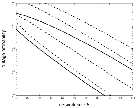
Figure 2: Outage probability for unicasting and multicasting via our two-phase protocol as a function of network size. The solid curves correspond to our Monte Carlo simulations, the dashed-dotted curves to our analytical approximations, and the dashed curves to our bounds. The top set of curves is for multicasting; the bottom set for unicasting. In the protocol we set $\beta=0.5$ and $R_{1}(\alpha)=R$, so that the rate is $R=(1/2)\log(1+P/(2N_{0}))<C$.

Remarks

1. First, the outage curves for both unicasting and multicasting approach zero with our cooperative protocol, which is a consequence of the transmission rate being below capacity. Note that, by contrast, for cooperation-free admissible protocols, the outage curves will not decay with network size.

2. Multicasting incurs significant penalty over unicasting in terms of outage probability for a fixed network size $K$. In particular, Fig. 2 confirms that the multicasting outage probability is indeed roughly a factor $K$ larger than the unicasting outage probability.

3. The slopes of the outage log-probability curves are asymptotically constant, and the bounds are good predictors of the asymptotic slopes. This is perhaps not surprising since we used Chernoff techniques to derive the bounds. Indeed, in many communication problems the Chernoff exponent is close to the correct exponent. However, the bounds are not particularly close to the the correct outage curves.

4. The analytical outage probability approximations are asymptotically quite close to the true curves, converging to within a factor of roughly 3 in probability for large network sizes. In addition, these approximations appear to be actual upper bounds at least in case study depicted, though this is conjecture.

5. The asymptotic slopes of the outage log-probability curves for both unicasting and multicasting are identical. In the next section, we will develop this slope as the network scaling exponent of the protocol, which we denote using $E_{\mathrm{ns}}^{-}$. For a target outage level, this slope can be used to quantify the asymptotic network size gap between unicasting and multicasting. In particular, suppose that for a fixed choice of $\alpha$ and $\beta$ in the protocol, $K^{\mathrm{uc}}(\epsilon)$ nodes are required to achieve some target outage probability $\epsilon$ in unicasting. Then the number of nodes required to achieve the same outage probability in multicasting is, asymptotically,

   $$K^{\mathrm{mc}}(\epsilon)=K^{\mathrm{uc}}(\epsilon)+\frac{1}{E_{{\mathrm{ns}}}^{-}}\log K^{\mathrm{uc}}(\epsilon).$$ (42)

   To verify (42), it suffices to recognize that the vertical distance between the unicasting and multicasting outage probabilities is, in accordance with (41), asymptotically, $\log K^{\mathrm{uc}}(\epsilon)$.

VII Network Scaling Exponent

In this section, we explore, in more detail, the asymptotic rate of decay of the outage probability with network size, which we have termed the network scaling exponent. This exponent captures meaningful information for system designers. For example, at the transmission rates to which Fig. 2 corresponds, outage probabilities for our two-phase protocol decay reasonably quickly in a practical sense — i.e., the network scaling exponent is reasonably large. However, as we will see, at rates close to capacity, it turns out that outage probabilities decay very slowly as a function of network size, corresponding to a small network scaling exponent. This implies that very large network sizes may be needed to achieve practical target error rates.

Before beginning our development, note that the network scaling exponent is the natural counterpart to the classical error exponent for traditional channel codes. In particular, the classical error exponent captures the exponential rate of decay of error probability with block length as a function of the the targeted fraction of capacity; see, e.g., [6]. Analogously, the network error exponent captures the exponential rate of decay of error probability in unicasting and multicasting with network size as a function of the targeted fraction of capacity.

Formal definitions follow.

Definition 4

The network reliability function with respect to a sequence of admissible protocols $\pi_{K}$ in Definition 1 is given by

$$E_{{\mathrm{ns}}}^{-}(\{\pi_{K}\})=-\lim_{K\rightarrow\infty}\frac{\ln\Pr\{{\mathcal{E}}_{\pi_{K}}\}}{K},$$ (43)

where ${\mathcal{E}}_{\pi_{K}}$ denotes the outage event for a system with $K$ nodes under the protocol $\pi_{K}$.

Definition 5

The network scaling exponent is the supremum of the network reliability functions of all sequences of admissible protocols with a rate that is at least a fraction $r$ of the capacity at a given SNR, i.e.,

$$E_{{\mathrm{ns}}}(r,\mathrm{SNR})=\sup_{\{\pi_{K}\}\in{\mathcal{P}}(r,\mathrm{SNR})}E_{{\mathrm{ns}}}^{-}(\{\pi_{K}\}),$$ (44)

where ${\mathcal{P}}(r,\mathrm{SNR})$ is a set of sequences of admissible protocols with a rate that is a fraction $r$ of the capacity.

The following establishes that, as with capacity, unicasting and multicasting are not distinguished by their network scaling exponents.

Proposition 3

The network scaling exponent is the same for both unicasting and multicasting.

Proof:

First, for any sequence of admissible protocols,

$$\Pr\{{\mathcal{E}}^{\mathrm{mc}}_{\pi_{K}}\}\geq\Pr\{{\mathcal{E}}^{\mathrm{uc}}_{\pi_{K}}\},$$

so that

$$E_{{\mathrm{ns}}}^{\mathrm{mc}}(r,\mathrm{SNR})\leq E_{{\mathrm{ns}}}^{\mathrm{uc}}(r,\mathrm{SNR}).$$ (45)

Furthermore, if $\{\pi^{*}_{K}\}$ achieves the supremum for the unicasting system, then from a simple application of the union bound it follows that, for each $K$,

$$\Pr\{{\mathcal{E}}^{\mathrm{mc}}_{\pi_{K}^{*}}\}\leq K\Pr\{{\mathcal{E}}^{\mathrm{uc}}_{\pi_{K}^{*}}\},$$

and hence

$$E_{{\mathrm{ns}}}^{\mathrm{mc}}(r,\mathrm{SNR})\geq E_{{\mathrm{ns}}}^{-,\mathrm{mc}}(\{\pi^{*}_{K}\})=E_{{\mathrm{ns}}}^{\mathrm{uc}}(r,\mathrm{SNR}).$$ (46)

Combining (45) and (46) we obtain $E_{{\mathrm{ns}}}^{\mathrm{mc}}(r,\mathrm{SNR})=E_{{\mathrm{ns}}}^{\mathrm{uc}}(r,\mathrm{SNR})$ as desired. ∎

In the remainder of this section, we analyze a lower bound on the network scaling exponent by optimizing over the class of the two-phase protocols described in Section V. For a fixed choice of $\alpha$ and $\beta$, we can express the fraction of the capacity achieved by the protocol as

$$r(\alpha,\beta,\mathrm{SNR})=\frac{R(\alpha,\beta,\mathrm{SNR})}{C(\mathrm{SNR})},$$ (47)

where we have made the dependency of both $R$ and $C$ in (14) and (3), on the parameters of interest explicit. We define the network reliability function of the user cooperation protocol in Section V as

$$E_{{\mathrm{ns}}}^{-}(r,\mathrm{SNR})=\sup_{\alpha,\beta:r(\alpha,\beta,\mathrm{SNR})\leq r}\left\{-\lim_{K\rightarrow\infty}\frac{\ln\Pr\{{\mathcal{E}}_{\alpha,\beta,K}\}}{K}\right\},$$ (48)

which constitutes a lower bound on $E_{{\mathrm{ns}}}(r,\mathrm{SNR})$ in (44). Note that in the above definition, we have constrained $\alpha$ and $\beta$ to be constants independent of $K$.

The upper envelope of the points in Fig. 3 indicates a lower bound on the network reliability function of our two-phase protocol. Each point in the plot corresponds to a particular choice of $\alpha$ and $\beta$ in the protocol, for which we have numerically evaluated $E_{{\mathrm{ns}}}^{-}$ in (48) for different values of $r$ at $\mathrm{SNR}=0$ dB.

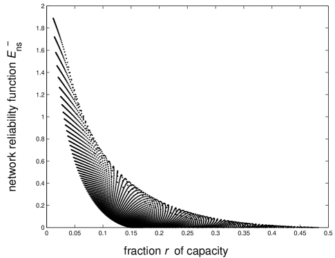
Figure 3: The upper envelope of the plotted points indicates the network scaling exponent for the two-phase cooperative protocol as a function of the targetted fraction of capacity $r$. Each point corresponds to a particular value of $\alpha$ and $\beta$. In this example, $\mathrm{SNR}=0$ dB.

Perhaps the most striking observation from Fig. 3 is that the error exponent for the two-phase protocol is quite small when aiming for rates that are more than about half of capacity. This implies that while the protocol is capacity achieving, it may require a prohibitively large number of nodes to achieve rates anywhere close to this capacity. It remains to be determined whether there exist more sophisticated protocols with substantially higher exponents in this regime.

As a final comment, it should also be noted that Fig. 3 effectively characterizes the efficient operating frontier for the protocol. In particular, given a network with $K$ nodes and an allowable outage probability $\epsilon$, one can approximate the scaling exponent by $-\ln\epsilon/K$ and determine the corresponding value of $r$, which is an estimate of how close one can expect to get to capacity in the system.

VIII Concluding Remarks

Perhaps the main contribution of this paper is a framework for analyzing user cooperation protocols in the limit of large network size (number of nodes), which we have illustrated in the case of a multipath-rich Rayleigh fading environment. Within this framework, we have introduced a meaningful notion of Shannon capacity for this regime and presented a simple two-phase protocol that can achieve rates arbitrarily close to capacity. A finer grain analysis of this two-phase protocol in terms of its network scaling exponent, which characterizes the rate of decay of error probabilty with network size, shows that it may require prohibitively large number of nodes to achieve rates close to the capacity with this protocol.

One important direction of future work is to study more sophisticated models beyond the Rayleigh fading model within our framework. One could for example incorporate the effects of network geometry and shadowing into the model. More generally, it would be of interest to study a class of channel models for which user cooperation plays a fundamental role in enabling reliable communication in multicasting. The Rayleigh fading model considered here clearly belongs to this class, but we believe the class may be quite rich and may include many other models of practical importance.

Another important direction is to investigate how system performance changes when the sum power constraint is replaced with individual power constraints. With individual power constraints, the system capacity will increase with the number of nodes — in fact, the MISO upper bound increases according to $\Theta(\log K)$. It remains to be determined whether there exist cooperative multicasting protocols that approach this upper bound or whether one can develop tighter upper bounds for this scenario.

Finally, as noted in Section VII, the two-phase protocol may require prohibitively large number of nodes to achieve rates close to the capacity. It remains to investigate whether more sophisticated protocols can improve the network scaling exponent substantially in this regime.

[Derivation of Outage Approximation (38)]

First, we write $\Pr\{{\mathcal{E}}^{\mathrm{uc}}_{\alpha,\beta,K}\}$ in the form

$$\Pr\{{\mathcal{E}}^{\mathrm{uc}}_{\alpha,\beta,K}\} =E\left[\Pr\{{\mathcal{E}}^{\mathrm{uc}}_{\alpha,\beta,K}|K_{1}\}\right]$$

$$=\sum_{k_{1}=1}^{K}\Pr\{K_{1}=k_{1}\}\,\Pr\{{\mathcal{E}}^{\mathrm{uc}}_{\alpha,\beta,K}\mid K_{1}=k_{1}\}$$

$$\approx\sum_{k_{1}=\alpha(1-\beta)K}^{K}\Pr\{K_{1}=k_{1}\}\,\Pr\{{\mathcal{E}}^{\mathrm{uc}}_{\alpha,\beta,K}\mid K_{1}=k_{1}\}.$$

Note that we have dropped the contribution of terms with $k_{1}\leq\alpha(1-\beta)K$ in the summation, since we expect their aggregate sum to be small as they deviate significantly from the mean $E[K_{1}]=\alpha K$.

We now approximate each of the two factors in (LABEL:eq:foo). The right factor we approximate by the upper bound (19). The left factor we replace with via Stirling’s approximation for binomial distributions [5, p. 284], yielding

$$\Pr\{K_{1}=k_{1}\} =\binom{K}{k_{1}}\alpha^{k_{1}}(1-\alpha)^{(K-k_{1})}$$

$$\approx\frac{1}{\sqrt{K}}\exp\left\{-KD\biggl{(}\frac{k_{1}}{K}\biggm{\|}\alpha\biggr{)}\right\},$$ (50)

where $D(\cdot\|\cdot)$ denotes the binary relative entropy function, i.e., for any $0<p,q<1$,

$$D(p\|q)\stackrel{{\scriptstyle\Delta}}{{=}}p\ln\frac{p}{q}+(1-p)\ln\frac{1-p}{1-q},$$ (51)

and where $\alpha$ is the parameter of $K_{1}$ (cf. (16)).

Thus, substituting (19) and (50) into (LABEL:eq:foo) yields

$$\Pr\{{\mathcal{E}}^{\mathrm{uc}}_{\alpha,\beta,K}\}$$

$$\approx\sum_{k_{1}=\alpha(1-\beta)K}^{K}\frac{1}{\sqrt{K}}\exp\left\{-KD\biggl{(}\frac{k_{1}}{K}\biggm{\|}\alpha\biggr{)}\right\}\quad\times$$

$$\quad\quad\quad\left(\frac{\alpha K(1-\beta)e}{k_{1}}\right)^{k_{1}}{\exp\left\{-\alpha K(1-\beta)\right\}}.$$ (52)

Finally, we approximate (52) by an approximation to the largest single term in the summation, viz.,

$$\Pr\{{\mathcal{E}}^{\mathrm{uc}}_{\alpha,\beta,K}\}\approx\frac{1}{\sqrt{K}}{\exp\left\{-\alpha K(1-\beta)\right\}}\quad\times\\ \qquad\max_{\gamma\in(\alpha(1-\beta),1)}\exp\left\{-KD(\gamma\|\alpha)+\gamma K\ln\left(\frac{\alpha(1-\beta)e}{\gamma}\right)\right\}.$$ (53)

Since the term in the exponent being minimized in (53) is differentiable and convex in $\gamma$, the optimizing $\gamma$ is the value at which the associated derivative is zero, i.e.,

$$\frac{\gamma^{2}}{1-\gamma}=\mu$$ (54)

where $\mu$ is as given in (40). Finally it is straightforward to verify that (54) has a solution in $(\alpha(1-\beta),1)$ and it may be solved explicitly, yielding (39).

References

- [1] K. Azarian, H. E. Gamal, and P. Schniter, “On the achievable diversity multiplexing tradeoff in half-duplex cooperative channels,” IEEE Trans. Inform. Theory, pp. 4152–72, 2005.
- [2] A. Bletsas, A. Khisti, D. Reed, and A. Lippman, “A simple cooperative diversity method based on network path selection,” IEEE J. Select. Areas Commun., To appear.
- [3] H. Boche and E. Jorswieck, “Outage probability in multiple antenna systems,” Euro. Trans. Telecom., To appear.
- [4] J. Canny, Combinatorics and Discrete Probability (CS174) Course Notes. Univ. Calif. Berkeley, http://www.cs.berkeley.edu/ jfc/cs174lecs/lec9/lec9.html.
- [5] T. M. Cover and J. A. Thomas, Elements of Information Theory. New York: Wiley, 1991.
- [6] R. G. Gallager, Information Theory and Reliable Communication. New York: Wiley, 1968.
- [7] B. M. Hochwald, T. L. Marzetta, and V. Tarokh, “Multiple-antenna channel hardening and its implications for rate feedback and scheduling,” IEEE Trans. Inform. Theory, vol. 50, pp. 1893–1909, Sep. 2004.
- [8] J. N. Laneman, D. N. C. Tse, and G. W. Wornell, “Cooperative diversity in wireless networks: Efficient protocols and outage behavior,” IEEE Trans. Inform. Theory, vol. 50, pp. 3062–80, Dec. 2004.
- [9] J. N. Laneman and G. W. Wornell, “Distributed space-time coded protocols for exploiting cooperative diversity in wireless networks,” IEEE Trans. Inform. Theory, vol. 59, pp. 2415–2525, Oct. 2003.
- [10] R. U. Nabar, H. Bölcskei, and F. W. Kneubühler, “Fading relay channels: Performance limits and space-time signal design,” IEEE J. Select. Areas Commun., pp. 1099–1109, Aug. 2004.
- [11] L. Ozarow, S. Shamai, and A. Wyner, “Information theoretic considerations for cellular mobil radio.” IEEE Trans. Vehic. Technol., vol. 43, no. 2, pp. 359–78, May 1994.
- [12] N. Prasad and M. K. Varanasi, “Diversity and multiplexing tradeoff bounds for cooperative diversity protocols,” in Proc. Int. Symp. Inform. Theory, Chicago, IL, June 2004, p. 268.
- [13] A. Sendonaris, E. Erkip, and B. Aazhang, “User cooperation diversity-Part I: System description,” IEEE Trans. Commun., vol. 51, pp. 1927–38, Nov. 2003.
- [14] E. Teletar, “Capacity of multi-antenna Gaussian channels,” Euro. Trans. Telecom., vol. 10, pp. 585–596, Nov./Dec. 1999.
- [15] D. Tse, P. Viswanath, and L. Zheng, “Diversity-multiplexing tradeoff in multiple access channels,” IEEE Trans. Inform. Theory, vol. 50, no. 9, pp. 1859–1874, Sep. 2004.
- [16] L. Zheng and D. Tse, “Diversity and multiplexing: A fundamental tradeoff in multiple antenna channels,” IEEE Trans. Inform. Theory, vol. 49, pp. 1073–1096, May 2003.