Understanding physics from interconnected data

Abstract

Metal melting on release after explosion is a physical system far from equilibrium. A complete physical model of this system does not exist, because many interrelated effects have to be considered. General methodology needs to be developed so as to describe and understand physical phenomena involved.

The high noise of the data, moving blur of images, the high degree of uncertainty due to the different types of sensors, and the information entangled and hidden inside the noisy images makes reasoning about the physical processes very difficult. Major problems include proper information extraction and the problem of reconstruction, as well as prediction of the missing data. In this paper, several techniques addressing the first problem are given, building the basis for tackling the second problem.

1 Introduction

Metal melting on release after explosion is considered here as an example of a physical system far from equilibrium. The goal is not only to describe and understand this system, but also to develop a more general methodology to approach similar problems. Due to the highly non-equilibrium nature of the process and the simultaneous interconnection of many different physical effects, a complete physical model of the process does not exist. Bayesian and correlational analysis of the data, as well as other data analysis methods, is a step in the direction of building the physical model. The ultimate task of this work is to find and utilize all possible dependencies within the system.

Metal melting on release possesses a number of different characteristics, some of which seem to be incompatible with each other. These include time, metal type, thickness of the material, etc. One can see that the problem of finding the physical model of the system is connected to the problem of combining its measurable properties in the case of minimal compatibility. Moreover, some of these characteristics, such as time and thickness, belong to a potentially infinite domain. On the other hand, being able to consider all the features of the system together is very important in understanding the underlying physical model.

Another important problem is the proper extraction of information from the raw experimental data. The extreme conditions of the environment restrict the choice of the sensors to use. Particularly, images are generated by proton radiography (PRAD) method. To achieve proper contrast, protons for each image are collected for a period of time that is relatively long, in comparison to the time scale of the physical phenomena, which in turn creates blurry, noisy, relatively low contrast proton-radiographic images (by typical standards of image processing). These images are a “gold mine” of the information essential to a specific goal; hence, feature extraction from the images is driven by the goal. On the other hand, they are significantly more difficult to process then usual images. Parameters like velocity of different parts of the system obtained from the images constitute the system representation. Standard image processing approaches, like gradient-based contour detection, however, can not be applied due to insufficient quality of the images. Other methods of contour detection and velocity calculations developed in the project are presented.

2 Experiment

Figure 1: Schematic representation of the experiment configuration.

The configuration of the experiment is given in figure 1. As seen in the figure, a metal coupon is connected to a high explosive (HE) cylinder 2-in. in diameter and 0.5-in. thick that is point initiated with a detonator centered on the charge. A VISAR probe is positioned 35-60 mm from the metal surface, whereas the center of the proton beam is 18-30 mm from the surface. The experimental data for this work were obtained from the research of D. B. Holtkamp et al Holtkamp and et al. (2003).

All considered experiments were performed under the same conditions, including the same type of high explosives with the point ignition positioned in the center, and the same diameter of metal coupons. In this paper, the work on tin samples of different thicknesses and their comparison is presented. Investigation of experiments with other types of metal and, possibly, with other types of ignition is the next step of this project.

2.1 Types of measurements

This work is based on two kinds of experimental data: numerical time series of velocities measured by VISAR that utilizes the Doppler effect of a laser beam Hemsing (1983), and time series of up to 20 images per experiment obtained using Proton Radiography (PRAD) Hogan and et al. (1999).

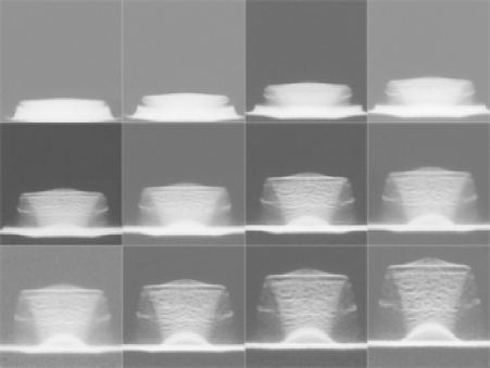
Figure 2: Structure evolution of the melting metal sample after explosion of 0.4375-in. thick coupon.

In figure 2, a series of PRAD images illustrating the melting during explosion (up to 57 usec ) of a 0.4375-in. thick coupon. The first image shows the coupon immediately after the ignition, while next images made approximately each 3 usec show the consecutive stages of the process. The data for each image were collected for 3.28 usec. Time series of images are very helpful in identifying different phases of the process. Note that a PRAD image is scaled in physical coordinates such that 1 pixel is equivalent to 0.01 mm².

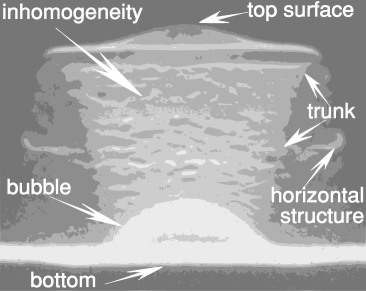
Figure 3: Main structures observed on a PRAD image. The image is captured about 50 usec after an ignition of 0.4375-in. thick tin coupon.

In figure 3, one can identify structures from the PRAD image of a melting coupon. The top surface could be solid in some experiments, while the bubble, together with the bottom, containing the majority of material, are always completely melted. In some experiments, the horizontal structure and inhomogeneity in the trunk area may be not present. The observed structure has axial symmetry due to the point ignition of the explosives, which is also responsible for the sheer waves observed in the material.

Figure 4: Time series of velocities measured by VISAR for tin coupons. The six series showed on the figure correspond to six different thicknesses in increasing order from top to bottom, ranging between 0.1875 and 0.5 inches.

Using VISAR, one can measure a velocity of the central point on the top surface. In figure 4, time series of such velocities corresponding to various thicknesses of the tin coupon are showed. As can be observed in figure 4, the thinnest coupon melted completely almost immediately after explosion, hence the VISAR reading came out very noisy (see the very top time series of the figure). Many observations can be linked to the increasing thickness of the coupon. For example, as the thickness increases, the average velocity decreases, the noise of the time series increases, the magnitude of the fluctuations increases, and the subsequent time before these fluctuations increases.

3 Problem

One of the main goals of this project is to quantify all possible information about the physical system underlying the experiment. At first, appropriate parameters should be identified and the relationships among them studied. These parameters include time and sample thickness. It is important to construct a data manifold Amari and Nagaoka (2000) in multidimensional data space that contains all the measured information at a single moment of time. Analysis of this data manifold evolution allows for the predictability of the system behavior on a longer time scale. Particularly, the missing data of one of the manifold’s dimensions (corresponding to one of the sensors) can be estimated via other fully specified data sets of the manifold. In a sense, a data manifold reflects the data and qualitative description of the system, and thus provides history in Bayesian reasoning.

It is important to make minimal theoretical assumptions while discovering the origins of the processes of the system and predicting their future behavior. In reality, assumptions about a model are unavoidable. However, tracing their influence on the results and understanding is crucial.

There are many different features of the given data that make the reasoning about the physical system difficult. These include gaps and uncertainty in the data due to the stochastic nature of the system. The given data is highly uneven, overlapped, and multidimensional. For instance, the VISAR data spans the initial period of time very densely, however at each time step it provides only a small amount of information. PRAD images, on the other hand, cover a longer period of time than VISAR data very sparsely, although, at each covered time step, a PRAD image provides a huge amount of information about many different parameters of the system. Data for one image is collected for a relatively long time (about 3.4 usec), taking into account that the speed of ejected metal is frequently of the order of 1km/s, while the time/space scale of physically interesting details is rather small.

Due to this large quantity of information in these images, image processing is essential. In addition to the difficulties of extraction of some information, even with cutting edge techniques, image processing is complicated because of specific features of PRAD imagery, including noise and granularity of the image, image blur, under- and over-shooting effects on the borders between different densities areas, scattering, and the fact that the axial symmetry assumption of PRAD makes non-cylindrical objects difficult to track.

Since the process being investigated is far from equilibrium, there is no direct way to measure thermodynamic quantities. These data can be obtained only under the assumption of an underlying numerical model, influencing the results and raise non-trivial questions about their credibility.

4 Methodology

The simplest way of analyzing different types of data describing one process is to work with each data type independently, due to the difficulty comparing essentially distinct sorts of data with significant error variability. However, it is strongly believed by the authors that besides considering parts of data, the data set must be analyzed as a whole in order to gain more knowledge of the process, especially in the presence of expensive, hard-to-repeat experiments. In particular, in order to solve the problem of data gaps, interpolation can be used. However, depending on the size of a gap, this approach might not produce the best solution. A higher-order analysis that accounts for the data from other sensors can be performed so as to capture the behavior of the process in the gap.

4.1 Image analysis

The goal of the first stage of the project is to gather information from the available data, a large portion of which is represented with images. Hence, image processing driven by the features of an image dictates further steps of the project.

In order to improve the performance of image analysis tools, the images are denoised. Since different parts of the same image require different amount of denoising, an additional heat-based denoising is performed.

Due to low contrast and high granularity of PRAD images, gradient-based contour detection methods perform poorly. As an alternative, the following method, called 1-bit erosion, is proposed. The gray scale image is converted into a 1-bit approximation by choosing a specific threshold. After eroding the black area one pixel deep and subtracting it from the 1-bit image, a continuous contour emerges (see figure 5).

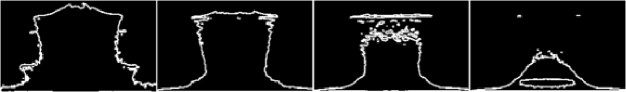
Figure 5: Different contours detected from a single PRAD image using 1-bit erosion method with the erosion threshold increasing from left to right.

The 1-bit erosion method, specially designed to extract contours from blurred images, is fast and robust. As can be seen in figure 5, one can catch contours of different structures of an image by choosing different erosion thresholds. However, the method is sensitive to the contrast of images: a threshold corresponding to a particular contour on one image corresponds to a different contour on the other image, and thus has to be adjusted manually. After performing contour detection on PRAD images, time series of contours are collected and analyzed (see figures 6 and 7).

Figure 6: Evolution of the top surface: the movement of the top surface from the bottom to the top in physical coordinates (left); the overlapped surfaces emphasizing the shape evolution (right). The axes correspond to physical coordinates. It can be seen that the central part of the top surface is moving slightly faster than the sides, which, however, does not tell whether the surface is melted or not.

Figure 7: Evolution of the bubble: the movement of the bubble from the bottom to the top in physical coordinates (left); the overlapped bubble surfaces emphasizing the shape evolution (right). It can be seen that bubble’s curvature is preserved, reflecting the shape of the initial shock wave.

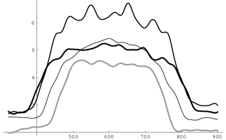
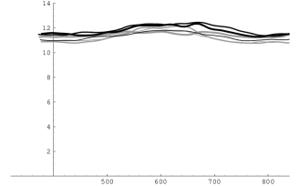
Figure 8: Changes in velocities of different parts of the system: velocities of the bubble (left); velocities of the top surface (right). For readability only five velocities are given. The time progresses from the gray line to the black one and from the thin one to the thick. The $x$-axis shows physical coordinates and the $y$-axis shows velocity.

Using the space and time coordinates, velocities of various parts of the system are calculated. In figure 8, one can see the velocities of the bubble and the top surface. As expected, the top surface moves faster than other parts of the system, while its center part evolves even faster. On the other hand, a semi-spherical shock wave approaches the center part of the building bubble first, and the bubble, as the wave progresses, grows up involving more and more area around itself.

5 Discussion

A complicated system composed of multiple processes, for which a mathematical model is not known, is frequently described by a set of various types of data measured by different sensors. In this paper, the experiment with melting of a tin coupon with different thickness is considered, making a first step towards the ultimate goal of understanding this physical system, which is equally important as developing a general methodology for analyzing and modeling its data.

So far the preliminary image analysis was performed on PRAD images, revealing the shape evolution of the system’s structures and their velocity fields. Consequently, the numerical time series (as opposed to series of images) are obtained that allow their comparison to the data from other sensors, such as VISAR.

There are two major future directions of the project that are closely related to each other: physical and numerical. The former concerns with the physical origins and phenomena of the system and creation of its physical model, while the later covers the numerical changes in the system and predictions of its further evolution. Potentially, there are several machine learning approaches to the numerical part of the project including Hidden Markov Models (HMMs) and Kalman Filters, Markov Networks and Ising Models (or even Cellular Automata). In particular, it seems interesting to attempt building and training HMM on VISAR data Chakrabarti et al. (2005) and then comparing HMM’s predictions with PRAD data.

References

- Holtkamp and et al. (2003) D. B. Holtkamp, and et al., “A Survey of High Explosive-Induced Damage and Spall in Selected Materials Using Proton Radiography,” in Shock Compression of Condensed Matter-2003, edited by M. D. Furnish, and et al., AIP Conference Proceedings 706, American Institute of Physics, New York, 2003, pp. 477–482.
- Hemsing (1983) W. F. Hemsing, “VISAR: Some Things You Should Know,” in SPIE Vol 427, edited by D. L. Paisley, SPIE, 1983, pp. 144–148.
- Hogan and et al. (1999) G. E. Hogan, and et al., “Proton Radiography,” in Particle Accelerator Conference, edited by A. Luccio, and W. MacKa, IEEE, Piscataway, 1999, vol. 1 of Particle Accelerator Conference Proceedings, pp. 579–583.
- Amari and Nagaoka (2000) S. Amari, and H. Nagaoka, Methods of Information Geometry, vol. 191 of Translations of Mathematical Monographs, American Mathematical Society, Oxford University Press, 2000, ISBN 0-8218-0531-2.
- Chakrabarti et al. (2005) C. Chakrabarti, R. Rammohan, and G. F. Luger, “A First-Order Stochastic Modeling Language for Diagnosis,” in FLAIRS Conference, edited by I. Russell, and Z. Markov, FLAIRS Conference Proceedings, AAAI Press, 2005, pp. 623–628.