The Signed Distance Function:
A New Tool for Binary Classification

Abstract

From a geometric perspective most nonlinear binary classification algorithms, including state of the art versions of Support Vector Machine (SVM) and Radial Basis Function Network (RBFN) classifiers, and are based on the idea of reconstructing indicator functions. We propose instead to use reconstruction of the signed distance function (SDF) as a basis for binary classification. We discuss properties of the signed distance function that can be exploited in classification algorithms. We develop simple versions of such classifiers and test them on several linear and nonlinear problems. On linear tests accuracy of the new algorithm exceeds that of standard SVM methods, with an average of 50% fewer misclassifications. Performance of the new methods also matches or exceeds that of standard methods on several nonlinear problems including classification of benchmark diagnostic micro-array data sets.

—————————————————
Machine Learning, Microarray Data
—————————————————

1 Introduction

Binary classification is a basic problem in machine learning with applications in many fields. Not only does binary classification have many potential direct applications, it is also the basis for many multi-category classification methods. Of particular interest are the applications in biology and medicine. The availability of micro-array and proteomic data sets that contain thousands or even tens of thousands of measurements have particularly made it important to develop good classification algorithms, since reliable use of these data could presumably revolutionize diagnostic medicine. Several binary classification algorithms have been developed and studied intensely over the past few years, most notable among these are the support vector machine (SVM) methods using radial basis functions and other functions as kernels. SVM methods have been shown to perform reasonably well in classifying micro-array data, demonstrating that the extraction of useful information from these large data sets is feasible.

We will begin in the next section with a geometric, rather than statistical, statement of the binary classification problem and our discussion will be restricted to the context of this geometric viewpoint. Nonlinear SVM methods, despite their geometric, maximal margin origin, have been developed based on the idea of reconstructing “indicator functions”, as discussed by Poggio and Smale [14]. RBFN methods are also currently employed in this way. The indicator function is an object that encodes only the most primitive geometric information. We propose that a potentially better tool for classification is the “signed distance function” (SDF), an intrinsically geometric object that has been employed in several areas of applied mathematics. The geometric properties of the SDF make it advantageous for use in classification and we give examples of how these properties can be exploited.

In this paper we also present preliminary test results for rudimentary implementations based on the idea of reconstructing the SDF from training data. We demonstrate that these non-optimized SDF-based algorithms outperform standard SVM (LIBSVM) methods on average by 50% (half as many misclassifications) on linearly separable problems. We also present a comparison of SDF classification with SVM method on the challenging geometric 4 by 4 checkboard problem in which the SDF-based method performs better. Finally, on 2 benchmark cancer-diagnosis micro-array data sets a nonlinear SDF algorithm performs just as well or better than highly-developed SVM methods. While these results are obviously not conclusive, they do demonstrate that the SDF paradigm is promising and worth further investigation.

2 A Geometric Formulation and a Geometric Tool

Suppose a set $X\subset{{\mathbb{R}}}^{n}$ is partitioned by $A\subset X$ and its complement $A^{c}$. The set $A$ might contain the set of test values that are associated with the presence of a disease, while $A^{c}$ contains those values that are not. For applications we may suppose that $A$ is a reasonably nice set, e.g. has a smooth boundary. The problem of binary classification is then to determine the set $A$ given a finite sample of data, i.e. for a set of points $\{x_{i}\}_{i=1}^{m}$ we know whether $x_{i}\in A$ or $x_{i}\in A^{c}$, for each $i$. The purpose of solving this problem is obviously predictive power; given a point $x\in X$ that is not among the given data $\{x_{i}\}_{i=1}^{m}$, we wish to determine if $x\in A$. In this paper we only consider this geometric formulation of the problem. While this formulation is obviously somewhat restrictive, it allows for geometric analysis and leads to a new class of methods that may be useful in some applications.

One way to approach this problem mathematically that is common among nonlinear classifiers is to consider the indicator function of $A$, $\iota_{A}:X\rightarrow\{-1,1\}$, defined by

$$\iota_{A}(x)=\begin{cases}\>1&\text{if $x\in A$,}\\ -1&\text{if $x\in A^{c}$.}\end{cases}$$ (1)

The known information is represented by $\{(x_{i},\iota_{A}(x_{i})\}_{i=1}^{m}$ and problem of binary classification is equivalent to reconstructing $\iota_{A}(x)$ from the data.

Current methods of binary classification such as the SVM methods and RBFN methods work by attempting to approximate the indicator function $\iota_{A}$ by regression over the known data, $\{(x_{i},\iota_{A}(x_{i})\}$. This was not the conceptual origin of the SVM, i.e. finding a separating plane of maximal margin, but is the basis for nonlinear “kernel trick” algorithms and efficient linear implementation as pointed out in [14]. In practice, the SVM constructed functions are smooth and $\pm 1$ are not the only values in the range, thus $x$ is interpreted as in $A$ if the constructed function is positive at $x$ and as being in $A^{c}$ if it is negative.

Rather than using the indicator function $\iota_{A}$, we propose using the signed distance function (SDF) of $A$, denoted $b_{A}(x)$ which is the distance to the boundary, $\partial A$, of $A$ if $x\in A$ or minus the distance to $\partial A$ if $x\in A^{c}$, i.e.

$$b_{A}(x)=\begin{cases}\;d(x,\partial A)&\text{if $x\in A$,}\\ -d(x,\partial A)&\text{if $x\in A^{c}$,}\end{cases}$$ (2)

where $d$ is a metric (distance function).

Knowledge of $b_{A}$ is obviously sufficient to fully determine the set $A$, it carries more information than $\iota_{A}$, and it has some smoothness. These and other properties can be used in classification and thus the SDF has advantages over the indicator function as a basis for binary classification algorithms. In fact we argue that SDF based classification, because it is more geometrical, is conceptually a more faithful generalization of the original SVM concept than existing nonlinear (kernel trick) SVM implementations.

Binary classification based on the SDF can work in much the same way as indicator function based classification; one attempts to approximate the function $b_{A}$ using only the given data. If the value of $b_{A}$ is positive at a test point $x$, then $x$ is predicted to be in $A$ and if the value is negative, $x$ is predicted to be in $A^{c}$. The approximation of $b_{A}$ can proceed similarly to that of $\iota_{A}$, i.e. by various forms of regression (including SVM and RBFN regression). A practical difference is that $\iota_{A}$ is given explicitly at the data points, whereas $b_{A}$ at the data points must be derived from the data. We investigate simple methods for doing this and show that they give reliable results. We also show that properties of $b_{A}$ can be used to refine those estimates. The complexity of this task is no worse than that needed to perform the regression itself, hence no computational performance is sacrificed.

3 Signed Distance Functions

In some places $b_{A}$ is called the oriented boundary distance function or the oriented distance function. Proofs of the following facts about $b_{A}$ can be found in [6].

Fact 1

The function $b_{A}$ is Lipschitz continuous, with Lipschitz constant $1$.

In other words, $|b_{A}(x)-b_{A}(y)|<|x-y|$, holds for all $x,y\in X$. This implies that $b_{A}(x)$ is differentiable almost everywhere, i.e, $Db_{A}(x)$ exists except on a set of zero measure. It also implies that $b_{A}(x)$ belongs to the Sobolev space $W^{1,p}_{loc}$ for any $1\leq p\leq\infty$.

Fact 2

If $b_{A}$ is differentiable at a point $x$, then there exists a unique $Px\in\partial A$ such that $b_{A}(x)=|x-Px|$ and

$$\nabla b_{A}(x)=\frac{Px-x}{b_{A}(x)}.$$

In the case it is unique, $Px\in\partial A$ is called the projection of $x$ onto $\partial A$. In particular, $|\nabla b_{A}(x)|=1$ and $Db_{A}(x)$ points from $x$ toward $Px$.

Fact 3

Let $A$ be a subset of ${{\mathbb{R}}}^{n}$ with nonempty boundary $\partial A$. Then $b_{A}$ is a convex function if and only if $\overline{A}$ is a convex set. If $A$ is convex, then $b_{A}$ is differentiable everywhere in $A^{c}$.

Fact 4

If $\partial A$ is of smoothness class $C^{k}$, i.e. it is $k$ times continuously differentiable, $k\geq 1$, then for each $y\in\partial A$ there is a neighborhood $V(y)$ of $y$ on which $b_{A}$ is a $C^{k}$ function.

If $\partial A$ is $C^{1}$, then at any point $y\in\partial A$ we can define the unit normal vector $n(y)$.

Fact 5

Suppose $\partial A$ is of smoothness class $C^{1}$ and $n(y)$ is Lipschitz continuous. At any point $y\in\partial A$, let $V(y)$ be as in Fact 4. Then for any $x\in V(y)$, $x=Px+b_{A}(x)n(Px)$.

In particular, $Px-x$ and $Db_{A}(x)$ are normal to $\partial A$ at $Px$.

Fact 6

Let $H_{y}$ denote the mean curvature of $\partial A$ at a point $y\in\partial A$. Then wherever $H_{y}$ exists it satisfies

$$H_{y}=\Delta b_{A}(x),$$

where $\Delta$ is the usual Laplace operator.

The function $b_{A}$ has been used in various branches of applied math such as free boundary problems [5, 7, 16, 18] and grid generation for finite-element methods [17]. It is intimately related to flow by mean curvature [6] and occurs in the solution of certain Hamilton-Jacobi partial differential equations [8, p. 163]. The geometric nature of the SDF connects it to well developed areas of geometry and analysis that can be expected to provide tools for both refinement and analysis of SDF based classification methods.

4 SDF Classifiers

4.1 Preliminary algorithms

In the SDF paradigm the input training data are marked as to class, but they do not come marked with the values $b_{A}(x_{i})$, and hence these need to be approximated. A naive SDF algorithm then consists of two simple steps, with an optional third refinement step.

• Approximate $b_{A}$ at the training data $\{x_{i}\}_{i=1}^{m}$. Denote these approximations by $\{b_{i}\}_{i=1}^{m}$

• Approximate $b_{A}$ by a function $B_{D}(x)$ on the entire domain through regression on $D:=\{(x_{i},b_{i})\}_{i=1}^{m}$.

• Use the constructed function $B_{D}$ and properties of $b_{A}$ to improve the estimates $\{b_{i}\}$ and iterate.

We now detail preliminary algorithms for these three steps and point to those areas that we consider important for further investigation.

4.2 Estimating $b_{A}$ at the data

Let $d$ denote a metric on $X\subset{{\mathbb{R}}}^{n}$. Usually we will let $d$ be the Euclidean metric, but we will also consider weighted distances. A reasonable and simple first approximation of $b_{A}$ at $\{x_{i}\}_{i=1}^{m}$ is given by

$$b_{i}=P^{\prime}(x_{i})\equiv\iota_{A}(x_{i})\cdot\min_{j\neq i}\{d(x_{i},x_{j}):\iota_{A}(x_{j})\neq\iota_{A}(x_{i})\},$$

i.e. the signed projection onto the (finite) data of opposite type. It is clear that $b_{i}$ has the correct sign and is a bound on $b_{A}(x_{i})$, i.e.

$$|b_{A}(x_{i})|\leq|b_{i}|.$$ (3)

It is easy to show by counter-example that obtaining more precise, yet rigorous, bounds on $b_{A}(x_{i})$ would require some assumptions on the shape of $A$. However, we can make some heuristic improvements in $\{b_{i}\}$. For instance, consider

$$\tilde{b}_{i}=b_{i}-b_{A}(P^{\prime}x_{i}).$$

Then we have

$$|b_{A}(x_{i})|\leq|\tilde{b}_{i}|\leq|b_{i}|.$$

Now suppose that $x_{i}\in A$ and $y_{i}\in A^{c}$ where $y_{i}$ is the closest data point to $x_{i}$ in $A^{c}$ and $x_{i}$ is the closest data point in $A$ to $y_{i}$. If $\partial A$ is situated half way between $x_{i}$ and $y_{i}$ and is normal to $y_{i}-x_{i}$, then $b_{A}(x)=d(x,y)/2$. Let $c_{i}$ denote the approximated signed distance of $y_{i}$ to the boundary, then we have:

$$b_{A}(x_{i})=\frac{1}{2}b_{i}=b_{i}-\frac{1}{2}c_{i}.$$

Then for any $x_{i}$ and $y_{i}=P^{\prime}x_{i}$ we define

$$b^{\prime}_{i}=b_{i}-.5c_{i}$$ (4)

where $b_{i}$ is the first approximation of $b_{A}(x_{i})$ and $c_{i}$ is the first approximation of $b_{A}(y_{i})$. It can be demonstrated that, on average, $b^{\prime}_{i}$ is a better approximation of $b_{A}(x_{i})$ than $b_{i}$.

4.3 Linear classifier

We will say that a binary classification problem in the context of our geometric formulation is linearly separable if $\partial A$ is a hyperplane in ${{\mathbb{R}}}^{n}$. In this case $b_{A}(x)$ will be a linear function whose zero set is $\partial A$. To use the SDF for a linearly separable problem one would seek a linear function as $B_{D}(x)$, i.e.

$$y=\ell(x)=w\cdot x+c=w_{1}x_{1}+w_{2}x_{2}+\ldots+w_{n}x_{n}+c$$

that fits the data $\{x_{i},b_{i})\}_{i=1}^{m}$. The most obvious choice for this approximation is to use the linear least squares approximation if $m>n$ or projection (pseudoinverse) if $m<n$, for which there are highly developed algorithms. In the linear tests below, we have used linear least squares regression.

From §2, we have $|\nabla b_{A}(x)|=1$ wherever it exists so we could let

$$|D\ell(x)|=|w|=1$$

be a constraint in the linear least squares approximation.

4.4 Nonlinear classifier

If the problem is not linearly separable, then $b_{A}(x)$ will be a nonlinear function. To approximate it we should use some form of nonlinear regression on $\{(x_{i},b_{i})\}_{i=1}^{m}$. There are many options for nonlinear regression that could be used, including SVM and RBFN regression algorithms. One simple, yet appealing, choice for the nonlinear regression is the least squares regression discussed in [14]. We implemented this approach in the nonlinear tests reported below and so we recall it.

Let $K:X\times X\rightarrow{{\mathbb{R}}}$ be a kernel that is symmetric ($K(x,y)=K(y,x)$) and positive-definite, i.e.,

$$\sum_{i,j=1}^{k}c_{i}c_{j}K(x_{i},x_{j})\geq 0,$$

for any $k$, any $x_{1},\ldots,x_{k}$ and any $c_{1},\ldots,c_{k}$. In the tests below we use the Gaussian

$$K(x,y)=e^{-d(x,y)^{2}/2\sigma^{2}},$$

which is symmetric and positive definite. Let $\mathbf{K}$ be the square, positive-definite matrix with elements $K_{i,j}=K(x_{i},x_{j})$. Let $\mathbf{I}$ be the identity matrix and $\mathbf{b}$ be the vector with coordinates $b_{i}$. Let $\gamma>0$ and let $\mathbf{c}$ be the solution of the linear system of equations:

$$(\mathbf{K}+m\gamma\mathbf{I})\mathbf{c}=\mathbf{b}.$$ (5)

This problem is well-posed since $(\mathbf{K}+m\gamma\mathbf{I})$ is strictly positive-definite and the condition number will be good provided that $m\gamma$ is not too small. The number $\gamma$ can be viewed as a smoothing parameter. Given the solution vector $\mathbf{c}$, the approximation, $B_{D}(x)$, of $b_{A}(x)$ is given by

$$B_{D}(x)=\sum_{i=1}^{m}c_{i}K(x_{i},x).$$

The choices of $\sigma$ and $\gamma$ in this approximation are discussed in [14] and elsewhere. In tests discussed below, results were insensitive to $\gamma$ within a fairly large range. Good choices for $\sigma$, which we found by cross-validation, were on the order of the mean inter-data distance.

We emphasize that other regression methods could be used in connection with SDF-based and should be investigated.

4.5 Iteration

There are some possibilities for refining the initial data approximation $\{b_{i}\}$. One idea for nonlinear problems would is to let

$$b^{\prime}_{i}=B_{D}(x_{i})$$

where $B_{D}$ is the regression obtained from $\{(x_{i},b_{i})\}$. Then one could take $b^{\prime}_{i}$ as a refinement of $b_{i}$ and then run the regression again. (For linear regression, this would repeat the original results.) We note that iterations of this type are related to the matrix eigenvalue problem for which there are well developed numerical techniques and which are amenable to stability analysis.

Another possibility is to use Facts 2 and 5 above to refine $b_{i}$. From these facts it is reasonable to project $y_{i}-x_{i}$ onto $Df(x_{i})$. This approach is particularly appealing for problems that are known a priori to be linearly separable. We have successfully implemented this iterative approach in the linear tests below, using the projection onto $w=D\ell$ to refine $\{b_{i}\}_{i=1}^{m}$.

5 Test Results

5.1 Linearly separable problems

We applied both non-iterative and iterative forms of the linear regression signed distance classifier to three types of distributions: uniform, normal and skewed. In all of these tests the linear SDF classifier decisively outperforms the linear classifiers in the LIBSVM package as well as the linear Lagrangian SVM [13] and the Proximal SVM [9].

A linearly separable problem can be transformed by a linear change of coordinate to the problem where $\partial A=\{x_{n}=0\}$. Thus we use this problem for our tests. We performed the tests for $n=2$. Data in the half space $x_{n}>0$ we labeled as in $A$ and data with $x_{n}<0$ we labeled as in $A^{c}$.

In the uniform distribution tests we let the domain be the square $[-1,1]\times[-1,1]\subset{{\mathbb{R}}}^{2}$. For the normal distribution we used the standard normal distribution at the origin in ${{\mathbb{R}}}^{2}$. For the skewed distribution, we randomly choose points in the square $[0,1]^{2}\subset{{\mathbb{R}}}^{2}$ using the density $\rho(x_{i})=1/\sqrt{x_{i}}$, then scaled them affinely to $[-1,1]^{2}$.

In the tests, we considered training sets of size from $m=10$ to $m=10,000$. For each $m$ in the range we classified 50 distributions of $m$ points. In each test we used a test set consisting of 4000 points selected randomly according to the distribution type being tested.

In Figures 1 we show comparisons of the SDF linear classifiers with the linear classifier from the LIBSVM along with the Lagrangian SVM [13] and Proximal SVM [9]. In this plot csvm and usvm are routines from the LIBSVM package, psvm is the Proximal SVM and lsvm is the Lagrangian SVM algorithm. In these tests the iterated SDF method was iterated 5 times. The iterated SDF method gave a 10% to 15% decrease in the error over the non-iterated SDF method. The Lagrangian method was also iterated 5 times. The LIBSVM package methods automatically iterate. In our trials, the number of iterations for the LIBSVM methods increased with $m$ and varied from 10 to 5000 iterations.

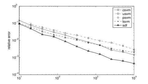
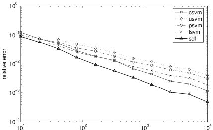
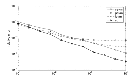
Figure 1: A comparison of classifiers on linearly separable data. In (a) the data are uniformly distributed, in (b) the data are normally distributed, and in (c) the data are from a skewed distribution. The $x$-axis is $\log(m)$, where $m$ is the number of data (training) points. Each point in the graph represents an average over 50 independent tests.

It can be seen that the SDF classifier has noticably smaller errors than either SVM method over a large range of number of training points $m$. Averaged over all 550 tests, the SDF-based classification produced 52% fewer misclassifications than the best SVM (LIBSVM c-SVM) method. (Average $\approx 98\%$ correct vs. $\approx 96\%$ correct).

5.2 The $4\times 4$ Checkerboard Problem

There are several benchmark nonlinear problems, but perhaps the prototype is the 4 by 4 checkerboard. This geometric problem is interesting because it is known to be difficult. In this test a square is partitioned into 16 equal sub squares with alternate squares belong to two distinct types, black or white (Figure 2). Following [13], we used 1,000 randomly selected points in each training set and 40,000 grid points as the test set.

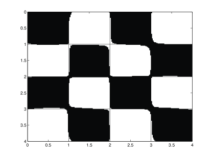
Figure 2: The 4 by 4 checkerboard problem classified by a nonlinear SDF-based classifier.

In Figure 3 we show the results of applying an SDF-based classification scheme and the standard LIBSVM package to 100 independent training set. We used the nonlinear least squares regression with parameters $\sigma$ and $\gamma$ found by cross-validation on the training sets. Parameters for the SVM classification were chosen by precisely the same process.

Note that the SDF-based method produces better results than the LIBSVM package. The mean correct % and standard deviation for the SDF method were 96.3% and .46%. For the SVM method the mean correct % was 94.5% with a standard deviation of .36%.

The standard deviation for our SDF method is slightly higher than that for the LIBSVM package. This is perhaps an artifact of our naive implementation of a SDF-based method.

We note that [13] reported $97.1\%$ accuracy on this problem using a Lagrangian SVM with 100,000 iterations.

Figure 3: Comparison of performance by the LIBSVM package and a SDF-based method on the four by four checkerboard problem.

5.3 Micro-array data sets

We compare the nonlinear SDF classifier with existing studies of SVM performance on two standard micro-array data sets involving cancer diagnosis. The first set, called Prostate–tumor, consists of 102 micro-array samples with 10,510 measurements each. Each patient represented by a sample was diagnosed independently for the presence of a prostate tumor. Of the 102 samples, 52 were from patients with a prostate tumor [20]. The second data set DLBCL consists of 77 samples with 5470 variables each. Samples were taken from patients diagnosed for a lymphoma. Of the 77 patients, 58 had Diffuse large B-cell lymphomas and 19 had follicular lymphomas [19].

With the two data sets, we tested the SDF nonlinear classifier with least squares regression on the data sets using Leave One Out Cross Validation (LOOCV). Accuracy of the LOOCV tests are shown in Table 1, with comparison of reported LOOCV performance from [22] using a variety of SVM methods and the k-nearest neighbor (KNN) method. The percentages reported are the percentages of correctly identified samples. It is important to point out that [22] showed that their error estimates did not change depending on the cross validation technique, and hence LOOCV is a robust estimate of performance when applied to these data.

Data set KNN SVM SDF Prostate–tumor $85\%$ $92.2\%$ $94.1\%$ DLBCL $87\%$ $97.4\%$ $97.4\%$

Table 1: Results from applying SDF-based classification to the benchmark DLBCL and Prostate–tumor micro-array data sets compared with the performance of SVM methods and the k-nearest neighbor method reported in [22]. All results are for Leave-one-out cross validation.

As seen in Table 1, the performance of the SDF classifier matches that of the SVM method on the DLBCL data and exceeds it on the Prostate–tumor data set.

In preliminary tests we found that performance on several LOOCV subsets once again was unaffected by $\gamma$ over a broad range $10^{-4}$–$10^{-12}$ . Based on this we simply set $\gamma=10^{-7}$ for the rest of the tests. Values for $\sigma$ were determined within each loop of the LOOCV process based on mean interdata distances for the subset. For the DLBCL data values of $\sigma$ were approximately $2.5\times 10^{4}$ and $\sigma$ was generally about $3.4\times 10^{3}$ for subsets of the Prostate–tumor set. For both of these data sets the optimal results are actually robust with respect to changes in the values of $\sigma$.

In these tests we used a weighted distance

$$d_{a}(x,y)=|a\cdot(x-y)|,$$

where $|\cdot|$ is the usual Euclidean norm and $a$ is a vector of weights. Distance functions of this type were shown to be effective in high dimensional binary classification problems in [2]. Specifically, we took $a$ to be the absolute values of the correlation coefficients relating each variable to the indicator on the data set. This was recalculated in the LOOCV process for each subset, independent of the excluded sample.

We note that in an independent set of experiments reported in [3], the nonlinear SDF-based classifier was compared to KNN, RBFN and SVM classifiers on five other cancer data sets. The following microarray data sets are involved: The Breast Cancer data set [24] consists of 49 tumor samples with 7129 human genes each. There are two different response variables in the data set: one describes the status of the estrogen receptor (ER), and the other one describes the status of the lymph nodal (LN), which is an indicator of the metastatic spread of the tumor. Of the 49 samples, 25 are ER+ and 24 are ER-, 25 are LN+ and 24 are LN-. The Colon Cancer data set [1] consists of 40 tumor and 22 normal colon tissues with 2000 genes each. The Leukaemia data set [10] consists of 72 samples with 7129 genes each. Each patient represented by a sample has either acute lymphoblastic leukemia (ALL) or acute myeloid leukemia (AML). Of the 72 samples, 47 are ALL and 25 are AML.

We tested the four classifiers in 100 independent trials on each of the data sets. In each trial, the data were divided randomly into a training set and a test set in a ratio of 2:1. We used Gaussian kernel functions for RBFN, SVM and SDF classifiers. For simplicity, we did not use any heuristic for the distance metrics of KNN, using the Euclidean distance. We claim that the classifiers are comparable in this setting since they are under exactly the same condition: (i) They share the same training set and test set in each trial, (ii) SVM and SDF share the same $\gamma=10^{-7}$, (iii) SVM uses the weighted kernel matrix returned by SDF in each trial, (iv) SVM and RBFN use the same $\sigma$, which is computed in each trial as the root mean square distance (RMSD) of the training data.

Data Set	KNN	RBFN	SVM	SDF
Breast cancer, ER	.0912	.0912	.0869	.0869
Breast cancer, LN	.2400	.2425	.2106	.2100
Colon cancer	.2200	.2143	.1700	.1662
Leukaemia	.0146	.0321	.0167	.0167

Table 2: Comparison of misclassification ratios averaged over 100 trials on randomly divided data.

Table 2 shows the test error rates averaged over the 100 independent trials for each classifier. KNN with $k=1,9,3,5$ neighbors achieves the best (in the averaging sense) generalization performance for the breast cancer data (ER), breast cancer data (LN), colon cancer data, and the leukemia data, respectively. Note that in actual use, $k$ would have to be determined in some unbiased way from the training data only. We note again that the naive SDF method matches or beats the SVM method on all data.

6 Discussion

In order to make the SDF paradigm competitive with indicator function based classification, the main need seems to be for more accurate, yet efficient, ways of obtaining an approximation of $b_{A}(x_{i})$. In the scheme we used in these tests, we simply search the entire data set for the closest point of the opposite type. In the worst case this takes $m^{2}$ operations, which is easily within the realm of practical computations. Increasing the accuracy of the approximation is a more difficult issue and should involve deeper geometric information from the data set.

In addition to better determination of $\{b_{i}\}$, use of other methods of nonlinear regression, including SVM and RBFN regression, with SDF-based classification should be explored. Another area for future exploration is development of iterative methods for the nonlinear classifier. We have described two possible procedures for this iteration and implemented one in a linear setting.

Smale and coworkers have been developing methods for rigorous estimates for the least squares regression algorithm outlined in §2.5. They produce these estimates in the framework of Reproducing Kernel Hilbert Spaces which have been shown to be isomorphic to certain Sobolev spaces [21], including the space $H^{1}_{loc}$, to which signed distance function are known to belong [6]. The estimates could be used in our context if the accuracy of the initial estimates $\{b_{i}\}_{i=1}^{m}$ are known. For the naive method of determining these values, an upper bound is given by (3) and we hope to obtain better bounds under assumptions on $A$. Other geometric methods for approximating $\{b_{i}\}_{i=1}^{m}$ should lend themselves to rigorous analysis depending on the methods. Perhaps for the case of iterative methods, the iteration process could be linked to known results in PDE and related functional analysis. Such a link would make an extremely rich arena of knowledge available for the purposes of estimates.

The above estimates of the approximated SDF should not only result in a overall reliability measure of the method, but should provide for any given test point an estimate of the distance of that test point from the decision surface. Combining this with statistical knowledge of the underlying application could provide a very natural “level of confidence” measure for any given test data. Such estimates would be especially useful in the context of biomedical applications.

There are concrete mathematical reasons why the SDF is a better basis than the indicator function for use in classification. The SDF is fundamentally geometric and this connects it solidly to geometric and analytical tools and methods. In preliminary tests, we have shown that a naive, non-optimized implementation of SDF-based classification is non-trivially more accurate than standard methods on geometric problems. In preliminary tests on nonlinear, high dimensional and noisy data, we have demonstrated that a non-optimized implementation of SDF is at least as accurate as current, standard SVM methods. These observations and results indicate that the SDF paradigm has the potential to be the basis for more accurate binary classification algorithms in many contexts.

References

- [1] U. Alon, N. Barkai, D. Notterman, K. Gish, S. Ybarra, D. Mack and A. Levine, Broad patterns of gene expression revealed by clustering analysis of tumor and normal colon tissues probed by oligonucleotide arrays, Proc. Natl. Acad. Sci 96 (1999), 6745-6750.
- [2] E. Boczko, T. Young, A. DiLullo, Binary classification based on potentials, Proceedings of The 2005 International Conference on Mathematics and Engineering Techniques in Medicine and Biological Sciences (METMBS’05: Las Vegas), 2005.
- [3] E. Boczko, T. Young, D. Wu and M.H. Xie, A comparison of signed distance function methods with SVM method on microarray data, preprint 2005.
- [4] J.P. Brody, B.A. Williams, B.J. Wold and S.R. Quake, Significance and statistical errors in the analysis of DNA microarray data, Proc. Nat. Acad. Sci. USA, 99 (2002), 12975-12978.
- [5] J. Cagnol and J.-P. Zolésio, Intrinsic geometric model for the vibration of a constrained shell, in Differential geometric methods in the control of partial differential equations (Boulder, CO, 1999), 23–39, Contemp. Math., 268, Amer. Math. Soc., Providence, RI, 2000.
- [6] M.C. Delfour and J.-P. Zolésio, Shape Analysis via Oriented Distance Functions, J. Functional Analysis 123 (1994), 129-201.
- [7] L.C. Evans and J. Spruck, Motion of level sets by mean curvature II, Trans. Amer. Math. Soc. 330 (1992), no. 1, 321–332.
- [8] L.C. Evans, Partial Differential Equations, GSM 19, Amer. Math. Soc., Providence, R.I., 1998.
- [9] G. Fung and O.L. Mangasarian, Proximal Support Vector Machine Classifiers, Preprint, 2001.
- [10] T. Golub, D. Slonim, P. Tomayo, C. Huard, M. Gaasenbeck, J. Mesirov, H. Coller, M. Loh, J. Downing, M. Caligiuri, C. Bloomfield, and E. Lander, Molecular classification of cancer: Class discovery and class prediction by gene expression monitoring, Science 286 (1999), 531-537
- [11] A. Krzyak, Nonlinear function learning using optimal radial basis function networks, Nonlinear Anal., 47 (2000), 293-302.
- [12] L.P. Li, C. Weinberg, T. Darden, L. Pedersen, Gene selection for sample classification based one gene expression data: study of sensitivity to choice of parameters of the GA/KNN method, Bioinformatics, 17 (2001), 1131-1142.
- [13] O.L. Mangasarian and D.R. Musicant, Lagrangian Support Vector Machines, J. Mach. Learn. Res., 1 (2001), no. 3, 161–177.
- [14] T. Poggio and S. Smale, The mathematics of learning: dealing with data, Notices Amer. Math. Soc., 50 (2003), no. 5, 537–544.
- [15] J.H. Moore, J.S. Parker, N.J. Olsen, Symbolic discriminant analysis of microarray data in autoimmune disease, Genet. Epidemiol., 23 (2002), 57-69.
- [16] S. Osher and R. Fedkiw, Level set methods and dynamic implicit surfaces, Applied Mathematical Sciences, 153, Springer-Verlag, New York, 2003.
- [17] P.O. Persson and G. Strang, A simple mesh generator in Matlab, SIAM Rev., 46 (2004), no. 2, 329–345.
- [18] J.A. Sethian, Level set methods. Evolving interfaces in geometry, fluid mechanics, computer vision, and materials science. Cambridge Monographs on Applied and Computational Mathematics, 3, Cambridge University Press, Cambridge, 1996.
- [19] M.A. Shipp, K.N. Ross, P. Tamayo, A.P. Weng, J.L. Kutok, R.C. Aguiar, M. Gaasenbeek, M. Angelo, M. Reich, G.S. Pinkus, T.S. Ray TS, M.A. Koval, K.W. Last, A. Norton, T.A. Lister, J. Mesirov, D.S. Neuberg, E.S. Lander, J.C. Aster, T.R. Golub, Diffuse large B-cell lymphoma outcome prediction by gene-expression profiling and supervised machine learning, Nat. Med. 8 (2002), 68-74.
- [20] D. Singh, P.G. Febbo, K. Ross, D.G. Jackson, J. Manola, C. Ladd, P. Tamayo, A.A. Renshaw, A.V. D’Amico, J.P. Richie, E.S. Lander, M. Loda, P.W. Kantoff, T.R. Golub, W.R. Sellers, Gene expression correlates of clinical prostate cancer behavior, Cancer Cell 1 (2002), 203-9.
- [21] S. Smale and D.X. Zhou, Learning theory estimates via integral operators and their approximations, preprint.
- [22] A. Statnikov, C.F. Aliferis, I. Tsamardinos, D. Hardin, S. Levy, A Comprehensive Evaluation of Multicategory Classification Methods for Microarray Gene Expression Cancer Diagnosis, Bioinformatics, to appear.
- [23] A. Statnikov, C.F. Aliferis, I. Tsamardinos. Methods for Multi-Category Cancer Diagnosis from Gene Expression Data: A Comprehensive Evaluation to Inform Decision Support System Development, in Proceedings of the 11th World Congress on Medical Informatics (MEDINFO), September 7-11, (2004), San Francisco, California, USA
- [24] M. West, C. Blanchette, H. Dressman, E. Huang, S. Ishida, R. Spang, H. Zuzang, J. A. Olson Jr, J. R. Marks, and J. R. Nevins, Predicting the Clinical Status of Human Breast Cancer by Using Gene Expression Profiles. (2001) Proc. Natl. Acad. Sci 98:11462-11467.