Carbon Copying Onto Dirty Paper

Abstract

A generalization of the problem of writing on dirty paper is considered in which one transmitter sends a common message to multiple receivers. Each receiver experiences on its link an additive interference (in addition to the additive noise), which is known noncausally to the transmitter but not to any of the receivers. Applications range from wireless multi-antenna multicasting to robust dirty paper coding.

We develop results for memoryless channels in Gaussian and binary special cases. In most cases, we observe that the availability of side information at the transmitter increases capacity relative to systems without such side information, and that the lack of side information at the receivers decreases capacity relative to systems with such side information.

For the noiseless binary case, we establish the capacity when there are two receivers. When there are many receivers, we show that the transmitter side information provides a vanishingly small benefit. When the interference is large and independent across the users, we show that time sharing is optimal.

For the Gaussian case we present a coding scheme and establish its optimality in the high signal-to-interference-plus-noise limit when there are two receivers. When the interference is large and independent across users we show that time-sharing is again optimal. Connections to the problem of robust dirty paper coding are also discussed.

I Introduction

The study of communication over channels controlled by a random state parameter known only to the transmitter was initiated by Shannon [21]. Shannon considered the case where the state sequence is known causally at the encoder. Subsequently, Gel’fand and Pinsker [10] analyzed the case where the state sequence is available noncausally. The noncausal model has found application in diverse areas, ranging from coding for memory with defects [18, 12], to digital watermarking [3, 4, 20], and to coding for the multiple-input/multiple-output (MIMO) broadcast channel [1, 25].

Costa [6] considered a version of the Gel’fand-Pinsker model in which there is an additive white Gaussian interference (“dirt”), which constitutes the state, in addition to independent additive white Gaussian noise. The key result in this “dirty paper coding” scenario is that there is no loss in capacity if the interference is known only to the transmitter.

By contrast, there has been very limited work to date on multiuser channels with state parameters known to the transmitter(s). In an early work in this area, Gel’fand and Pinsker [11] show that the Gaussian broadcast channel with independent messages incurs no loss in capacity if the interference sequences are known noncausally to the transmitter. Some other multiuser settings are also discussed. The degraded broadcast channel with independent messages and state sequence known to the transmitter either causally or non-causally is examined in [23]. Other works on multiuser channels with state parameters include [17], [2],[16],[13] and [22].

This paper examines the common-message broadcast channel, which we refer to as the multicast channel. Specifically, we consider a scenario in which one transmitter broadcasts a common message to multiple receivers. In addition to additive noise, associated with the link to each receiver is a corresponding additive interference. The collection of such interferences is thus the (random) state of the multiuser channel. In our model, the transmitter has perfect noncausal knowledge of all these interference sequences, but none of the receivers have knowledge of any of them. This model and its generalizations arise in a variety of multi-antenna wireless multicasting problems as well as in applications of robust dirty paper coding where only imperfect knowledge of the state is available to the transmitter.

The capacity of some binary versions of such multicast channels is reported in [14],[15]. For more general channels, [24] reports achievable rates for broadcasting common and independent messages over a discrete memoryless channel with noncausal state knowledge at the transmitter. The case of two-user Gaussian channels with jointly and individually independent identically distributed (i.i.d.) Gaussian interferences on each link is also considered in [24], for which it is conjectured that in the limit of large interference, time-sharing between the two receivers is optimum even when both are only interested in a common message. Among other results, in this paper we establish that this conjecture is true. We upper bound the capacity of the Gaussian channel and show that it approaches the time-sharing rate in this limit. In addition, we also present a coding scheme that is asymptotically optimal in the limit of high signal-to-interference-plus-noise (SINR) ratio .

An outline of the paper is as follows. Section II presents the general multicast channel model of interest. The binary special cases of interest are analyzed in Section III, and the Gaussian special cases of interest are analyzed in Section IV. Finally, Section V contains some conclusions and directions for future work. The proofs of the converses are deferred to the Appendices.

II Multicast Channel Model

The $K$-user multicast channel of interest is defined as follows.

Definition 1

A $K$-user discrete memoryless multicast channel with random parameters consists of an input alphabet ${\mathcal{X}}$, output alphabets ${\mathcal{Y}}_{1},{\mathcal{Y}}_{2},\dots,{\mathcal{Y}}_{K}$ for receivers $1,2,\dots,K$, respectively, and a state alphabet ${\mathcal{S}}$. For a given state sequence $s^{n}=(s_{1},s_{2},\dots,s_{n})$ such that $s_{i}\in{\mathcal{S}}$ and input $x^{n}=(x_{1},x_{2},\dots,x_{n})$ such that $x_{i}\in{\mathcal{X}}$, the channel outputs are distributed according to

$$p(y_{1}^{n},y_{2}^{n},\dots,y_{K}^{n}|x^{n},s^{n})=\prod_{i=1}^{n}p(y_{1i},y_{2i},\dots y_{Ki}|x_{i},s_{i})$$ (1)

where $y_{k}^{n}=(y_{k1},y_{k2},\dots,y_{kn})$, for all $y_{ki}\in{\mathcal{Y}}_{k}$, $k=1,2,\dots,K$. Moreover, $p(s^{n})=\prod_{i}p(s_{i})$. The particular realization $s^{n}$ is known noncausally to the transmitter before using the channel, but not to any of the $K$ receivers.

It is worth emphasizing that the above definition includes the case where the channel of User $k$ is controlled by its own state $s_{k}^{n}$. In such cases, the joint state is, with slight abuse of notation, $s^{n}=(s_{1}^{n},s_{2}^{n},\dots,s_{K}^{n})$, so that $p(s_{i})=p(s_{1i},s_{2i},\dots,s_{Ki})$.

The capacity of the channel of Definition 1 is defined as follows.

Definition 2

A $(2^{nR},n)$ code consists of a message set ${\mathcal{W}}_{n}=\{1,2,\dots 2^{nR}\}$, an encoder $f_{n}:{\mathcal{W}}_{n}\times{\mathcal{S}}^{n}\rightarrow{\mathcal{X}}^{n}$, and $K$ decoders $g_{k,n}:{\mathcal{Y}}_{k}^{n}\rightarrow{\mathcal{W}}_{n}$ for $k=1,\ldots,K$. The rate $R$ is achievable if there exists a sequence of codes such that for $W$ uniformly distributed over ${\mathcal{W}}_{n}$ we have

$$\lim_{n\rightarrow\infty}P_{e}^{n}=\lim_{n\rightarrow\infty}\Pr\left\{\bigcup_{k=1}^{K}\{g_{k,n}(Y_{k}^{n})\neq W\}\right\}=0.$$ (2)

Note that the error probability in (2) is averaged over all state sequences and messages. The capacity $C$ is the supremum of achievable rates.

In the remainder of the paper, we focus on special cases of the memoryless channel in Definition 1. In particular, we focus on binary and Gaussian cases in which the state is an additive interference; for results on the memory with defects multicast channel, see, e.g., [14].

III Noiseless Binary Case

We first consider the noiseless binary special case of Definition 1. Specifically, the channel outputs $Y_{1}^{n},Y_{2}^{n},\dots,Y_{K}^{n}$ depend on the input $X^{n}$ and the states $S_{1}^{n},S_{2}^{n},\dots,S_{K}^{n}$ according to

$$Y_{k}^{n}=X^{n}\oplus S_{k}^{n}$$ (3)

where $X_{i},S_{ki}\in\{0,1\}$, and $\oplus$ denotes symbol-by-symbol modulo-two addition (i.e., exclusive-or). In (3), the memoryless case of interest corresponds to the requirement that the $(S_{1i},S_{2i},\dots,S_{Ki})$ for $i=1,2,\dots,n$ form an i.i.d. sequence of $K$-tuples. In particular, for each $i$ the variables $\{S_{1i},S_{2i},\dots,S_{Ki}\}$ may in general be statistically dependent, and do not need to be identically distributed. As a result, we express our results in terms of the properties of a generic $K$-tuple in this sequence, which we denote by $(S_{1},S_{2},\dots,S_{K})$.

Note that with only a single receiver ($K=1$), the capacity is trivially 1 [bit per channel use], which is achieved by interference precancellation, i.e., by choosing $X^{n}=S^{n}\oplus B^{n}$, so that $Y^{n}=B^{n}$, where $B^{n}$ is the bit representation for the message $W$. As we will now develop, when there are multiple receivers, capacity is generally less than this ideal single-user rate.

III-A The Case of $K=2$ Receivers

The case of two receivers, which is depicted in Fig. 1, is the simplest nontrivial scenario since perfect interference precancellation is not possible simultaneously for both users.

\psfrag{&0}{$W$}\psfrag{&1}{Encoder}\psfrag{&3}{$X^{n}$}\psfrag{&4a}{Decoder 1}\psfrag{&4b}{Decoder 2}\psfrag{&5a}{$Y_{1}^{n}$}\psfrag{&5b}{$Y_{2}^{n}$}\psfrag{&6a}{$\hat{W}_{1}$}\psfrag{&6b}{$\hat{W}_{2}$}\psfrag{&7a}{$S_{1}^{n}$}\psfrag{&7b}{$S_{2}^{n}$}\includegraphics[width=234.87749pt]{figs/noiseless.eps}

Figure 1: Two-user memoryless, noiseless binary multicast channel with additive interference. The encoder maps message $W$ into codeword $X^{n}$. The state takes the form of interference sequences $S_{1}^{n}$ and $S_{2}^{n}$. Each channel output $Y_{k}^{n}=X^{n}\oplus S_{k}^{n}$, where $\oplus$ denotes symbol-by-symbol modulo-two addition, is decoded to produce message estimate $\hat{W}_{k}$.

One lower bound on the two-user capacity corresponds to a time-sharing approach that precancels the interference of one of the receivers at a time, yielding a rate of $R_{\mathrm{TS}}=1/2$. Another lower bound corresponds to ignoring the interference at the transmitter, i.e., treating each of the channels as a binary symmetric channel. This strategy yields a rate of $R_{\mathrm{IS}}=1-\max\{H(S_{1}),H(S_{2})\}$. It turns out that the former bound is only tight when $S_{1}$ and $S_{2}$ are independent and ${\mathcal{B}}(1/2)$, and the latter bound is only tight when both $S_{1}$ and $S_{2}$ are ${\mathcal{B}}(0)$.

A coding theorem for the channel is as follows.

Theorem 1

The capacity of two-user noiseless, memoryless binary channel with additive interference is given by

$$C=1-\frac{1}{2}H(S_{1}\oplus S_{2}).$$ (4)

Proof:

A converse is provided in Appendix A. The achievability argument is detailed below:

1. Select $2^{nR}$ codewords randomly according to an i.i.d. ${\mathcal{B}}(1/2)$ distribution in a codebook ${\mathcal{C}}$ of rate $R$ strictly less than the capacity (4). Denote these codewords as $B^{n}(1),B^{n}(2),\ldots,B^{n}(2^{nR})$, so a message $w$ is represented by codeword $B^{n}(w)$.

2. Select a sequence $A^{n}$ by flipping a fair coin for each symbol index (the realization of which is also known at the decoders [26]). Select the set ${\mathcal{A}}_{1}$ of symbol indices where $A_{i}=1$, and precancel the interference at those indices for user 1, and precancel the interference at the remaining indices ${\mathcal{A}}_{2}$ (with $A_{i}=0$) for user 2. Specifically, the transmitted sequence is of the form

   $$X_{i}(w)=\begin{cases}B_{i}(w)\oplus S_{1i}&i\in{\mathcal{A}}_{1}\\ B_{i}(w)\oplus S_{2i}&i\in{\mathcal{A}}_{2}.\end{cases}$$ (5)

With this encoding, receiver 1 then observes a version of $B^{n}(w)$ where $|{\mathcal{A}}_{1}|$ symbols are correct, and the remaining $|{\mathcal{A}}_{2}|$ symbols are corrupted by interference $S_{1i}\oplus S_{2i}$, $i\in{\mathcal{A}}_{2}$, corresponding to a binary symmetric channel with crossover probability $q^{\prime}=\Pr\{S_{1}\oplus S_{2}=1\}$. Receiver 2 experiences the opposite effect. Thus for large $n$ we have, since $|{\mathcal{A}}_{1}|/n\rightarrow 1/2$,

$$\frac{1}{n}I(B^{n};Y_{k}^{n}|A^{n})\rightarrow\frac{1}{2}+\frac{1}{2}(1-H(S_{1}\oplus S_{2})),\quad k=1,2,$$ (6)

which is $C$ in (4). As the mutual information expression in (6) indicates, the decoding of $Y_{k}^{n}$ to the message $\hat{W}_{k}$ is done by using the knowledge of ${\mathcal{A}}_{1}$ and ${\mathcal{A}}_{2}$ (i.e., $A^{n}$) at the decoders. In particular, receiver 1 selects a codeword which agrees with the received symbols in the set ${\mathcal{A}}_{1}$ and which is typical with noise $S_{1}\oplus S_{2}$ with the symbols in the set ${\mathcal{A}}_{2}$. For decoder 2, the order of the sets is reversed. As long as $R\leq C$, $\hat{W}_{k}$ equals $W$ with high probability. ∎

Fig. 2 shows the performance gains of optimal coding relative to time-sharing and disregarding the side-information. In particular, the achievable rate in the case of independent interferences is plotted as a function of the strength of the interference as measured by $q=\Pr\{S_{1}=1\}=\Pr\{S_{2}=1\}$.

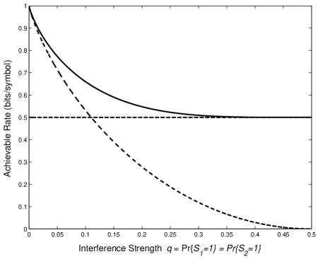
Figure 2: Achievable rates for the two-user noiseless binary multicast channel with independent and identically distributed interferences, as a function of the strength of the interference. Capacity is indicated by the solid curve, time-sharing performance is indicated by the horizontal dashed line, and the performance of a system that ignores the side information is indicated by the downward sloping dashed curve.

Three immediate conclusions can be drawn from Theorem 4. First, transmitter-only side information incurs a penalty relative to system-wide side information unless $S_{1}$ and $S_{2}$ are completely dependent random variables, i.e., unless $S_{2}=S_{1}$ or $S_{2}=\overline{S_{1}}$. Second, time-sharing is strictly sub-optimal except when $S_{1}$ and $S_{2}$ are independent ${\mathcal{B}}(1/2)$ random variables. We emphasize that, by contrast, when there are independent messages for each of the receivers in Fig. 1, time-sharing between the receivers is optimal and there is no loss in the capacity region with side information only at the transmitter. Finally ignoring the side information at the transmitter is strictly suboptimal except when $H(S_{1})=H(S_{2})=0$.

We make a few additional observations.

Some Further Remarks

1. The achievability argument can also be obtained via a different, more direct, but perhaps less intuitive route as follows. First note that a straightforward extension of the random binning argument for the single user case [10] shows that the following rate is achievable for the $K$-user multicast channel with random parameters.

   $$R_{K}=\max_{p(U|S),p(X|U,S)}\{\min_{k}I(U;Y_{k})-I(U;S)\},$$ (7)

   Here $U$ is an auxiliary random variable (over some alphabet ${\mathcal{U}}$) that satisfies the Markov constraint $U\leftrightarrow(X,S)\leftrightarrow Y_{k}$ for $k=1,2,\dots,K$.

   For the two-user binary channel, the following choice of $U$ yields the achievability of (4). Let the alphabet of $U$ be ${\mathcal{U}}=\{\Psi_{1},\Psi_{2},\Psi_{3},\Psi_{4}\}$.

   $$U =A\,\{\Psi_{1}\,(X\oplus S_{1})+\Psi_{2}\,(\overline{X\oplus S_{1}})\}$$ (8)

   $$\quad+\bar{A}\,\{\Psi_{3}\,(X\oplus S_{2})+\Psi_{4}\,\overline{(X\oplus S_{2})}\},$$

   where, $X$ is ${\mathcal{B}}(1/2)$ random variable, independent of $S_{1}$ and $S_{2}$, and $A$ is also ${\mathcal{B}}(1/2)$ that is independent of $X$, $S_{1}$ and $S_{2}$, and where $\bar{\cdot}$ denotes the complement of a (binary-valued) variable.

2. For the code construction outlined above suggests the transmitter does not require noncausal knowledge of the interference. We emphasize, however, this result is specific to the noiseless binary channel model.

3. It is straightforward to verify that random linear codes are sufficient to achieve the capacity of Theorem 4. It suffices to use an argument analogous to that used by Gallager for the binary symmetric channel [9, Sec. 6.2].

4. Theorem 4 can be readily generalized to the case of state sequences that are not in general i.i.d. In this case the term $H(S_{1}\oplus S_{2})$ in (4) is simply replaced with the entropy rate of $S_{1}^{n}\oplus S_{2}^{n}$.

5. Our achievability scheme also applies in the presence of noise. For the channel model

   $$Y_{1} =X\oplus S_{1}\oplus Z_{1}$$

   $$Y_{2} =X\oplus S_{2}\oplus Z_{2},$$

   where $Z_{1}$ and $Z_{2}$ are mutually independent and identically distributed Bernoulli random variables and independent of all other variables, we can show that a rate

   $$R=1-\frac{1}{2}H(S_{1}\oplus S_{2}\oplus Z_{1})-\frac{1}{2}H(Z_{1})$$

   is achievable and an upper bound is given by

   $$R^{+}=1-\frac{1}{2}H(S_{1}\oplus S_{2})-\frac{1}{2}H(Z_{1})$$

   Note that time-sharing is optimal in the special case when $S_{1}$ and $S_{2}$ are independent ${\mathcal{B}}(1/2)$ random variables.

III-B The Case of $K>2$ Receivers

When there are more than two receivers further losses in capacity ensue, as we now develop. Specifically, we have the following bounds on capacity.

Theorem 2

The capacity of the $K$-user noiseless binary channel in which the generic $S_{1},S_{2},\dots,S_{K}$ are mutually independent and identically distributed is bounded according to:

$$R_{-}\leq C\leq R_{+},$$ (9a)

where

$$R_{+} =1-\frac{1}{K}H(S_{1}\oplus S_{2},S_{1}\oplus S_{3},\ldots,S_{1}\oplus S_{K}),$$ (9b)

$$R_{-} =\max\left\{1-H(S_{1}),1-\left(1-\frac{1}{K}\right)H(S_{1}\oplus S_{2})\right\}.$$ (9c)

Proof:

The upper bound (9b) is established in Appendix B. The lower bound (9c) is obtained via a direct generalization of the code construction (5) in the case of two users. Specifically, it suffices to consider a code construction that divides each codeword into $K$ equally sized blocks and precancels the interference for a different user in each of the blocks. Each user then experiences one clean block and $K-1$ noisy blocks governed by a binary symmetric channel with crossover probability $q^{\prime}=\Pr\{S_{1}\oplus S_{2}=1\}$ as before. ∎

In general, the lower and upper bounds in (9) do not coincide. However, the associated rate gap decreases monotonically with the number of receivers $K$. Moreover, even for $K=3$, it is small, as Fig. 3 illustrates.

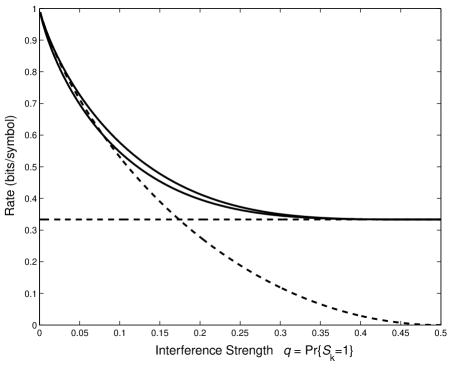
Figure 3: Upper bound and lower bounds on the capacity of the three-user noiseless binary multicast channel, as a function of the strength of the interference. The solid curves depict the two bounds of (9). The horizontal dashed line indicates the performance of time-sharing, while the other dashed curve indicates the performance of a strategy in which the side information is ignored by the transmitter.

The rate gap also decays to zero in the limit of large $K$, which follows readily from Theorem 9. In particular, $C\rightarrow 1-H(S)$ as $K\rightarrow\infty$, where $S$ denotes a generic random variable with the distribution of the $S_{k}$. To see this, it suffices to recognize that when $S_{1},S_{2},\dots,S_{K}$ are i.i.d.,

$$\left(1-\frac{1}{K}\right)H(S) \leq\frac{1}{K}H(S_{1}\oplus S_{2},S_{1}\oplus S_{3},\dots,S_{1}\oplus S_{K})$$ (10)

$$\leq H(S).$$

As $K\rightarrow\infty$, the lower and upper bounds in (10) converge, so that the upper bound on capacity (9b) converges to $R_{+}=1-H(S)$. However, this rate is achievable by simply treating the interference as noise at the receivers, so it is the limiting capacity. It should be emphasized that this implies that when the number of receivers is large, the side-information available to the transmitter is essentially useless.

We can also use (10) to bound the rate penalty associated with ignoring side information as a function of the number of receivers $K$. In particular, the gap is at most $H(S)/K$.

Finally, we can use Theorem 9 to establish that in the limit of large interference, time-sharing is optimal for every $K$. Specifically, when $S_{k}\sim{\mathcal{B}}(1/2)$, the capacity is $C=1/K$ and is achieved through time-sharing. To see this, it suffices to specialize the upper bound in (9b). Specifically, $S_{1}\oplus S_{k}$ for $k=2,3,\dots,K$ are independent ${\mathcal{B}}(1/2)$ random variables, so the joint entropy is $K-1$.

IV Gaussian Case

In this section we consider a memoryless Gaussian extension of Definition 1 and incorporate an average power constraint on the input. Unless otherwise stated, we restrict to the two-user ($K=2$) case. In the scenario of interest, depicted in Fig. 4, the state is additive, and the associated interferences $S_{k}^{n}$ are zero-mean white Gaussian sequences of power $Q$. We first focus on the case of independent interferences and consider the case of correlated interferences in section IV-A. In addition, each receiver’s link also has a zero-mean additive white Gaussian noise $Z_{k}^{n}$ of power $N$. Thus, the observation at receiver $k$ takes the form

$$Y_{k}^{n}=X^{n}+S_{k}^{n}+Z_{k}^{n},\qquad k=1,2.$$ (11)

Our power constraint takes the form

$$\frac{1}{n}E\left[\sum_{i=1}^{n}X_{i}^{2}(W,S_{1}^{n},S_{2}^{n})\right]\leq P,$$ (12)

where the expectation is taken over the ensemble of messages and interference sequences. Finally, note that without loss of generality, we may set $N=1$, and interpret $P$ as the signal-to-noise ratio (SNR), and $Q$ as the interference-to-noise ratio (INR).

\psfrag{&0}{$W$}\psfrag{&1}{Encoder}\psfrag{&3}{$X^{n}$}\psfrag{&4a}{Decoder 1}\psfrag{&4b}{Decoder 2}\psfrag{&5a}{$Y_{1}^{n}$}\psfrag{&5b}{$Y_{2}^{n}$}\psfrag{&6a}{$\hat{W}_{1}$}\psfrag{&6b}{$\hat{W}_{2}$}\psfrag{&7a}{$S_{1}^{n}$}\psfrag{&7b}{$S_{2}^{n}$}\psfrag{&8a}{$Z_{1}^{n}$}\psfrag{&8b}{$Z_{2}^{n}$}\includegraphics[width=234.87749pt]{figs/gaussian.eps}

Figure 4: Two-user Gaussian multicast channel model with additive interference. The encoder maps message $W$ into codeword $X^{n}$. The state takes the form of interference sequences $S_{1}^{n}$ and $S_{2}^{n}$. Each channel output $Y_{k}^{n}=X^{n}+S_{k}^{n}+Z_{k}^{n}$ is decoded to produce message estimate $\hat{W}_{k}$. . The interference and noise sequences are i.i.d. and mutually independent. Furthermore, $S_{1},S_{2}\sim{\mathcal{N}}(0,Q)$ and $Z_{1},Z_{2}\sim{\mathcal{N}}(0,1)$.

For this channel, we present the following bounds on the capacity.

Theorem 3

An upper bound on the Gaussian multicast channel capacity is :

$$C\leq\min\{R_{+}^{\mathrm{I}},R_{+}^{\mathrm{II}}\},$$ (13)

where ^,

$$R_{+}^{\mathrm{I}}=\begin{cases}\frac{1}{4}\log(1+P)+\frac{1}{4}\log\left(\frac{P+Q+1+2\sqrt{PQ}}{Q}\right)&Q\geq 4\\ \frac{1}{4}\log\left(\frac{1+P}{Q/4+1}\right)+\frac{1}{4}\log\left(\frac{P+Q+1+2\sqrt{PQ}}{Q/4+1}\right)&Q<4\end{cases}$$ (14)

$$R_{+}^{\mathrm{II}}=\begin{cases}\frac{1}{2}\log\left(\frac{1+P+Q+2\sqrt{PQ}}{1+Q/2}\right)&Q\leq 2\\ \frac{1}{2}\log\left(\frac{1+P+Q+2\sqrt{PQ}}{\sqrt{2Q}}\right)-\left[\frac{1}{4}\log\left(\frac{Q}{2P+2}\right)\right]^{+}&Q>2\end{cases}$$ (15)

We have presented two different upper bounds denoted by $R_{+}^{\mathrm{II}}$ and $R_{+}^{\mathrm{I}}$ since neither bound dominates the other, over all values of $(P,Q)$. The two bounds have been derived by slightly different methods. The bound $R_{+}^{\mathrm{I}}$ is obtained by observing that the channel is non-trivial even if we set one of the interferences (say $S_{1}$) to 0. Furthermore, it is possible to show that an upper bound on this modified channel is also an upper bound on the Gaussian multicast channel of interest. A complete derivation of this upper bound is presented in Appendix D. The expression for $R_{+}^{\mathrm{II}}$ is obtained by directly applying a chain of inequalities on the Gaussian multicast channel and its derivation is presented in Appendix C.

We remark here that the upper bounds are explicit expressions of the following maximization:

$$R_{+}^{\mathrm{I}} =\min_{\rho\in[-1,1]}\frac{1}{4}\log\left(\frac{1+P}{1+\rho}\right)+\frac{1}{4}\log\left(\frac{P+Q+1+2\sqrt{PQ}}{Q/2+1-\rho}\right)$$ (16)

$$R_{+}^{\mathrm{II}} =\min_{\rho\in[-1,1]}\frac{1}{2}\log\left(\frac{P+Q+2\sqrt{PQ}+1}{\sqrt{(1+\rho)(Q+1-\rho)}}\right)$$ (17)

$$\quad-\left[\frac{1}{4}\log\left(\frac{Q}{2P+(1+\rho)}\right)\right]^{+}$$

Theorem 4

A lower bound on the Gaussian multicast channel capacity is :

$$R_{-}=\begin{cases}\frac{1}{2}\log\left(1+\frac{P}{Q/2+1}\right)&Q/2<1\\ \frac{1}{2}\log\left(\frac{P+Q/2+1}{Q}\right)+\frac{1}{4}\log\left(\frac{Q}{2}\right)&1\leq Q/2<P+1\\ \frac{1}{4}\log(1+P)&Q/2\geq P+1.\end{cases}$$ (18)

Proof:

The lower bound (18) is an explicit expression of the following maximization:

$$R_{-}=\max_{\{(P_{A},P_{D}):P_{A}\geq 0,P_{D}\geq 0,P_{A}+P_{D}\leq P\}}R(P_{A},P_{D})$$ (19a)

with

$$R(P_{A},P_{D})\stackrel{{\scriptstyle\Delta}}{{=}}\frac{1}{2}\log\left(1+\frac{P_{A}}{P_{D}+Q/2+1}\right)+\frac{1}{4}\log\left(1+P_{D}\right).$$ (19b)

Accordingly, we show the achievability of (19b). The proposed scheme, combines superposition coding, dirty paper coding, and time-sharing, and exploits a representation of the interferences in the form

$$S_{1}^{n} =A^{n}+D^{n}$$ (20)

$$S_{2}^{n} =A^{n}-D^{n},$$

where

$$A^{n} =(S_{1}^{n}+S_{2}^{n})/2$$ (21)

$$D^{n} =(S_{1}^{n}-S_{2}^{n})/2.$$

We list the main steps for codebook generation, encoding and decoding. The probability of error analysis will be omitted as it is based on standard typicality arguments. See e.g. [7].

Codebook Generation: The idea is to generate three codebooks. There is one common codebook which both the users share and two private codebooks which are intended for the corresponding user. More specifically we follow the following steps:

1. Decompose the message $W$ into two submessages $W_{A}$ and $W_{D}$ and divide the power $P$ into two powers $P_{A}$ and $P_{D}$ so that $P=P_{A}+P_{D}$. Message $W_{A}$ will be decoded by both the receivers while message $W_{D}$ will be decoded by only one receiver at a time. We will transmit it twice so that both the receivers can decode (see encoding and decoding rules below for a further description).

2. Generate a codebook ${\mathcal{C}}_{A}$ for $W_{A}$ where the codewords $U_{A}^{n}$ are sampled from i.i.d. a Gaussian distribution $U_{A}=X_{A}+\alpha_{A}A$. Here $X_{A}$ is Gaussian ${\mathcal{N}}(0,P_{A})$, independent of $A$ and $\alpha_{A}=P_{A}/(P+Q/2+1)$. A total of $2^{nI(U_{A};Y_{i})}$ codewords are thus generated and randomly partitioned into $2^{nI(U_{A};A)}$ bins. The rate of this codebook, $I(U_{A};Y_{i})-I(U_{A};A)$ can be shown to be :

   $$R_{A}=\frac{1}{2}\log\left(1+\frac{P_{A}}{P_{D}+Q/2+1}\right).$$ (22)

3. Generate two codebooks ${\mathcal{C}}_{D}^{(1)}$ and ${\mathcal{C}}_{D}^{(2)}$ for $W_{D}$ for the two receivers as follows. For ${\mathcal{C}}_{D}^{(1)}$, the codewords $U_{D}^{n}$ are sampled from a i.i.d.  Gaussian distribution $U_{D}=X_{D}+\alpha_{D}((1-\alpha_{A})A+D)$, where $X_{D}$ is Gaussian ${\mathcal{N}}(0,P_{D})$, independent of $A$ and $D$ and $\alpha_{D}=P_{D}/(P_{D}+1)$. Generate $2^{nI(U_{D};Y_{1},U_{A})}$ such codewords and partition them into $2^{nI(U_{D};A,D)}$ bins. Follow analogous construction for codebook ${\mathcal{C}}_{D}^{(2)}$. The rate of each codebook $I(U_{D};Y_{i},U_{A})-I(U_{D};A,D)$ can be shown to be:

   $$R_{D}=\frac{1}{2}\log(1+P_{D}).$$ (23)

Encoding: We transmit a superposition of two sequences corresponding to $W_{A}$ and $W_{D}$ as follows:

1. To encode a message $W_{A}$, find a codeword $U_{A}^{n}$ in the bin of $W_{A}$, such that $X_{A}^{n}=U_{A}^{n}-\alpha_{A}A^{n}$ satisfies a power constraint of $P_{A}$. By construction, such a codeword exists with high probability.

2. To encode $W_{D}$, we decide whether to send it to user 1 or 2. The users are served alternately. When we decide to send it to user 1, we select a codeword $U_{D}^{n}$ in the bin of codebook ${\mathcal{C}}_{D}^{(1)}$ corresponding to message $W_{D}$ such that $X_{D}^{n}=U_{D}^{n}-\alpha_{D}\{(1-\alpha_{A})A^{n}+D^{n}\}$ satisfies a power constraint of $P_{D}$. When we decide to transmit to user 2, we select a codeword $U_{D}^{n}$ in the bin of codebook ${\mathcal{C}}_{D}^{(2)}$ corresponding to message $W_{D}$ such that $X_{D}^{n}=U_{D}^{n}-\alpha_{D}\{(1-\alpha_{A})A^{n}-D^{n}\}$ satisfies the power constraint of $P_{D}$. Since there are $2^{nI(U_{D};A,D)}$ codewords in each bin, such a codeword exists with high probability.

3. Send the superposition $X^{n}=X_{A}^{n}+X_{D}^{n}$, which has power $P$, over the channel.

Decoding: The decoding exploits successive cancellation (stripping) and proceeds as follows:

1. Decode $U_{A}^{n}$ from $Y_{1}^{n}$ or $Y_{2}^{n}$ treating $X_{D}^{n}$ as part of the noise. The received signals are of the form

   $$Y_{1}^{n} =X_{A}^{n}+A^{n}+(D^{n}+Z_{1}^{n}+X_{D}^{n})$$

   $$=U_{A}^{n}+(1-\alpha_{A})A^{n}+(D^{n}+Z_{1}^{n}+X_{D}^{n}),$$

   $$Y_{2}^{n} =X_{A}^{n}+A^{n}+(-D^{n}+Z_{2}^{n}+X_{D}^{n})$$

   $$=U_{A}^{n}+(1-\alpha_{A})A^{n}+(-D^{n}+Z_{2}^{n}+X_{D}^{n}).$$

   Since $D^{n}+Z_{i}^{n}+X_{D}^{n}$ is an i.i.d. Gaussian ${\mathcal{N}}(0,P_{D}+Q/2+1)$ sequence, independent of $A^{n}$, our choice of rate $R_{A}$ in (22) ensures that the resulting $\hat{W}_{A}$ equals $W_{A}$ with high probability at both the receivers.

2. Subtract the decoded $U_{A}^{n}$ from each of $Y_{1}^{n}$ and $Y_{2}^{n}$, so that the residual signals $\tilde{Y}_{i}^{n}=Y_{i}^{n}-U_{A}^{n}$ are of the form

   $$\tilde{Y}_{1}^{n} =X_{D}^{n}+((1-\alpha_{A})A^{n}+D^{n})+Z_{1}^{n},$$ (24)

   $$\tilde{Y}_{2}^{n} =X_{D}^{n}+((1-\alpha_{A})A^{n}-D^{n})+Z_{2}^{n}.$$ (25)

   The rate $R_{D}$ in (23) ensures that $U_{D}^{n}$ can be decoded from either $\tilde{Y}_{1}^{n}$ or $\tilde{Y}_{2}^{n}$ so that the resulting $\hat{W}_{D}$ equals $W_{D}$ with high probability at the corresponding receiver. Specifically, for the fraction of time that the transmitter encodes $W_{D}$ for interference $(1-\alpha_{A})A^{n}+D^{n}$, user 1 can recover $W_{D}$, while for the fraction of time that the transmitter encodes $W_{D}$ for interference ${(1-\alpha_{A})A^{n}-D^{n}}$, user 2 can recover $W_{D}$.

From this coding strategy, we see that the average rate delivered to each receiver is identical, i.e., $R_{A}+(1/2)R_{D}$. Maximizing this rate over the choices of $P_{A}$ and $P_{D}$ subject to the constraint $P=P_{A}+P_{D}$ optimizes the lower bound, whence (19a).

∎

From (18), we obtain several useful insights. First, note that in the high INR regime ($Q/2\geq P+1$), our lower bound reduces to time-sharing, while in the low INR regime ($Q/2\leq 1$) it reduces to dirty paper coding with respect to $A^{n}$. In the moderate interference regime, our bound shows that one can generally achieve a gain over these two strategies by a superposition coding approach that combines them.

The behavior of the bounds as a function of INR is depicted in Fig. 5 for a fixed SNR of $P=33$ dB. When the INR is very small ($Q\ll 1$), Fig. 5 reflects the rather obvious fact that the side information can be ignored by the transmitter without sacrificing rate. Similarly, when the INR is large($Q\gg 1$), Fig. 5 reflects that time-sharing between the two users achieves the capacity. More generally,

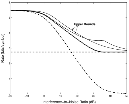
Figure 5: Upper and lower bounds on the capacity of the two-user Gaussian multicast channel, as a function of INR $Q$ for an SNR $P=33$ dB. The upper two curves depict the two upper bounds from (15) and (14). The marked line is the achievable rate in (18). The horizontal dashed line indicates the performance of time-sharing, while the other dashed curve indicates the performance of a strategy in which the side information is treated by the transmitter as additional noise on each link.

.

$$\lim_{Q\rightarrow\infty}C\leq\lim_{Q\rightarrow\infty}R_{+}^{\mathrm{I}}=\lim_{Q\rightarrow\infty}R_{+}^{\mathrm{II}}=\frac{1}{4}\log(1+P),$$ (26)

which can be achieved by time-sharing between the two users and doing Costa dirty paper coding for each user being served. We note that this result settles the conjecture made in [24].

Perhaps more interestingly, our proposed achievable rate is optimal in the limit of high SINR. The behavior of the bounds as a function of SNR is depicted in Fig. 6 for a fixed INR of $Q=15$ dB. We note that the expression for $R_{+}^{\mathrm{II}}$ coincides with $R_{-}$ in this limit. Note that the base-line schemes do not achieve a rate particularly close to capacity, but the superposition dirty paper coding strategy corresponding to our lower bound does. More generally, we can show that:

$$\lim_{P\rightarrow\infty}(C-R_{-}) \leq\lim_{P\rightarrow\infty}(R_{+}^{\mathrm{II}}-R_{-})=0$$ (27)

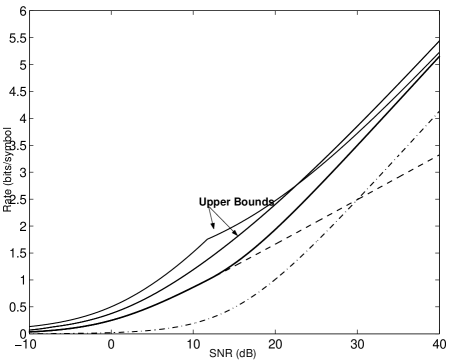
Figure 6: Upper and lower bounds on the capacity of the two-user Gaussian multicast channel, as a function of SNR $P$ for an INR $Q=15$ dB. The upper two curves depict the two upper bounds in (15) and (14). The achievable rate in (18) is also shown. The dashed curve indicates the performance of time-sharing, while the dash-dotted curve indicates the performance of a strategy in which the side information is treated by the transmitter as additional noise on each link.

To verify (27) for $Q\geq 2$, since $P\rightarrow\infty$, the middle case of the lower bound (18) applies which we can alternately express in the form

$$R_{-}=\frac{1}{2}\log\left(\frac{P+Q/2+1}{\sqrt{2Q}}\right)$$ (28)

Comparing (28) with the upper bound (15) we have

$$R_{+}^{\mathrm{II}}-R_{-} =\frac{1}{2}\log\frac{P+Q+1+2\sqrt{PQ}}{\sqrt{2Q}}$$ (29)

$$\quad-\frac{1}{2}\log\frac{P+Q/2+1}{\sqrt{2Q}},$$

which in the limit $P\rightarrow\infty$ gives (27). The case $Q\leq 2$, can be similarly verified. We summarize the optimality properties in the following corollary.

Corollary 1

For the Gaussian multicast channel in Figure 4, the proposed achievable rate in Theorem 4 is optimal in the limit of high SINR ($P\rightarrow\infty,Q$ is fixed). For $Q>2$ it can be expressed as $C(P)=\frac{1}{2}\log\left(\frac{P}{\sqrt{2Q}}\right)+o(1)$, where $o(1)\rightarrow 0$ as $P\rightarrow\infty$. For $Q\leq 2$ it can be expressed as $C(P)=\frac{1}{2}\log\left(\frac{P}{1+Q/2}\right)+o(1)$. Finally, for the case of fixed $P$ and $Q\rightarrow\infty$, time-sharing between the two users is optimal and the capacity can be expressed as $C(P)=\frac{1}{4}\log(1+P)+o(1)$, where $o(1)\rightarrow 0$ as $Q\rightarrow\infty$.

Finally, we show in Appendix C-B that a universal constant that bounds the difference between our upper and lower bounds is given by:

$$\sup_{P,Q}R_{+}^{\mathrm{II}}-R_{-}=\frac{1}{2}\log\left(\frac{3}{2}+\sqrt{2}\right)=0.7716$$ (30)

We conclude this section with a few additional observations.

Some Further Remarks

1. Extension to K receivers: Our upper bounding technique for $R^{\mathrm{II}}_{+}$ in (15) can be extended to the case of $K$ receivers each with independent interference. We show in Appendix C-C that the following upper bound holds for the case of $K$ receivers:

   $$R^{K}_{+} \leq\frac{1}{2}\log(P+Q+1+2\sqrt{PQ})-\frac{K-1}{2K}\log Q$$ (31)

   $$\quad-\frac{1}{2K}\log K-\left[\frac{1}{2K}\log\left(\frac{Q}{K(P+1)}\right)\right]^{+}$$

   By taking the limit $Q\rightarrow\infty$ in (31), it can be sown that time-sharing is optimal for any number of users in the high INR limit.

2. Correlation between noise sequences: The upper bound in Theorem 3 is valid even when the noises $Z_{1}^{n}$ and $Z_{2}^{n}$ are not independent. The argument is analogous to that for the standard broadcast channel (e.g. [7, Ch. 14]). We exploit this observation to derive the upper bound expressions. Furthermore analogous to the result in [4], even if the noise is not Gaussian our lower bound in (19a) is achievable when the decoder treats the noise as Gaussian.

3. Feedback does not help much. As discussed in Appendix C-A and D-A, the expressions for $R_{+}^{\mathrm{I}}$ and $R_{+}^{\mathrm{II}}$ in (16) and (17) continue to hold in the presence of perfect causal feedback, provided we do not optimize over the parameter $\rho$, but set it to equal the actual correlation between the noise terms.

4. The capacity-achieving strategy for the binary channel does not extend immediately to the Gaussian channel. While one might speculate that an adaptation of the achievability approach in Theorem 4 for the Gaussian channel would improve on the lower bound (19a) in Theorem 4, the obvious generalizations do not. In particular, strategies which precancel the interference in part of the codeword for each user achieved lower rates than our superposition dirty paper coding; for a further discussion see [14].

IV-A Correlated Interferences and Robust Dirty Paper Coding

Consider the a memoryless Gaussian point-to-point channel model with output

$$Y^{n}=X^{n}+{S}^{n}+Z^{n},$$ (32)

where $X^{n}$ is the channel input subject to power constraint $P$, ${S}^{n}$ is a white Gaussian interference sequence of power $Q$ not known to decoder, and $Z^{n}$ is a white Gaussian noise sequence of unit power. When the interference ${S}^{n}$ is perfectly known to the encoder, Costa’s dirty paper coding is capacity achieving. However, in many applications, only imperfect knowledge of ${S}^{n}$ is available to the encoder. One special case is the case of causal knowledge considered by Shannon. Another is the case of noisy noncausal knowledge. For these kinds of generalizations, there is interest in understanding the capacity of such channels and the structure of the associated capacity-achieving codes, which we refer to as robust dirty paper codes.

It is often natural to analyze such problems via their equivalent Gaussian multicast model. As an illustration, suppose that the interference in (32) is of the form ${S}^{n}=\beta S_{0}^{n}$ where $S_{0}^{n}\thicksim{\mathcal{N}}(0,Q{\mathbf{I}})$ is known to the encoder but $\beta$ is not. Then if $\beta$ is from a finite alphabet (or can be approximated as being so), i.e., $\beta\in\{\beta_{1},\beta_{2},\dots,\beta_{K}\}$, the problem is equivalent to a Gaussian multicast problem with $K$ users where the interference for the $k$th user is $\beta_{k}S_{0}^{n}$.

From this example it is apparent that for at least some applications, there is a need to accommodate correlated interferences in the Gaussian multicast model. In what follows we focus on that case where there are two receivers i.e. $\beta\in\{\beta_{1},\beta_{2}\}$. Extensions to the case of more than two receivers are possible, but will not be explored.

We first provide a general upper bound for the case of correlated, jointly Gaussian interference sequences and then specialize it to the case of scaled interferences. The general upper bound might be of independent interest and is derived in Appendix E.

Theorem 5

Consider a two receiver channel model $Y_{i}^{n}=X^{n}+S_{i}^{n}+Z^{n}$ for $i=1,2$ when $Z^{n}$ is i.i.d. ${\mathcal{N}}(0,1)$ noise, $S_{1}^{n}$ and $S_{2}^{n}$ are i.i.d. jointly Gaussian with marginal distributions ${\mathcal{N}}(0,Q_{1})$ and ${\mathcal{N}}(0,Q_{2})$ respectively and suppose that the distribution of $S_{1}-S_{2}$ is ${\mathcal{N}}(0,Q_{d})$. An upper bound on the common message rate for this channel under a power constraint $P$ at the transmitter is given by:

$$\ R_{+}^{\mathrm{C}}=\sum_{i=1}^{2}\frac{1}{4}\log(P+Q_{i}+1+2\sqrt{PQ_{i}})-T(Q_{d})$$ (33)

where

$$T(Q_{d})=\begin{cases}\frac{1}{4}\log(Q_{d}),&Q_{d}>4\\ \frac{1}{2}\log\left(1+\frac{Q_{d}}{4}\right),&Q_{d}\leq 4\end{cases}$$ (34)

We note that the upper bound is of most interest in the high signal-to-interference-plus-noise limit i.e. when we fix $Q_{1}$,$Q_{2}$ and take $P\rightarrow\infty$. In this limit we have the following:

Corollary 2

In the high SINR limit ($Q_{1},Q_{2}$ fixed, $P\rightarrow\infty$), the upper bound on the case of correlated interferences in Theorem 34 can be written as

$$R_{+}^{\mathrm{C}}=\frac{1}{2}\log(P)-T(Q_{d})+o(1),$$ (35)

where the term $o(1)$ approaches 0 as $P\rightarrow\infty$ and $Q_{1},Q_{2}$ fixed and $T(Q_{d})$ is given in (34).

To establish an achievable rate, we will consider a modification to our lower bound in Theorem 4 which considers the case of independent interferences. To deal with the case of correlated interferences, we will require that the encoder and decoders have access to a common source of randomness which will be used as a dither sequence.

Consider a superposition dirty paper coding strategy analogous to that in the proof of the lower bound in Theorem 4, whereby we decompose the interferences according to (20). In this case, we have that (21) specializes to

$$A^{n} =\beta_{A}\,S_{0}^{n}$$ (36)

$$D^{n} =\beta_{D}\,S_{0}^{n},$$

where

$$\beta_{A} =(\beta_{1}+\beta_{2})/2$$ (37)

$$\beta_{D} =(\beta_{1}-\beta_{2})/2.$$

When we turn to implement the encoding step in the proof of the lower bound of Theorem 4, in which $A^{n}$ is treated as interference and $D^{n}$ as noise, the results of [6] cannot be directly applied since the interferences $A^{n}$ and $D^{n}$ in (36) are correlated. On the other hand, if we assume that the encoder and decoder(s) have access to a source of common randomness in the form of a dither sequence, we can use the lattice coding strategy in [8]. In this scheme, the transmitted sequence is statistically independent of the interference and noise sequences. It can be easily shown that for such schemes, correlation between the interference and noise sequences does not change the achievable rate relative to the case when the noise and interference sequences are independent . With this scheme, we obtain the following lower bound.

Theorem 6

An achievable rate for our example multicast channel with correlated interferences and common randomness at the encoder and decoders is given by:

$$C^{\beta}(P)\geq\max_{\{(P_{A},P_{D}):P_{A}\geq 0,P_{D}\geq 0,P_{A}+P_{D}\leq P\}}R^{\beta}(P_{A},P_{D}),$$ (38a)

where

$$R^{\beta}(P_{A},P_{D}) =\frac{1}{2}\log\left(1+\frac{P_{A}}{1+Q_{d}/4+P_{D}}\right)$$ (38b)

$$\quad+\frac{1}{4}\log\left(1+P_{D}\right).$$

where $Q_{d}\stackrel{{\scriptstyle\Delta}}{{=}}(\beta_{1}-\beta_{2})^{2}Q$ is the variance of $S_{1}-S_{2}$.

Optimizing over $P_{A}$ and $P_{D}$, gives the following achievable rate:

$$R_{-}^{\beta}(P)=\begin{cases}\frac{1}{2}\log\left(1+\frac{P}{1+Q_{d}/4}\right),&Q_{d}<4\\ \frac{1}{2}\log\left(\frac{P+1+Q_{d}/4}{\sqrt{Q_{d}}}\right),&4\leq Q_{d}\leq 4(P+1)\\ \frac{1}{4}\log(1+P),&Q_{d}\geq 4P+4\end{cases}$$ (39)

We note that in the limit of high SINR, our expression for $R_{-}^{\beta}$ in (39) is given by $R_{-}^{\beta}=\frac{1}{2}\log(P)-T(Q_{d})+o(1)$, where $T(Q_{d})$ is given as in (34). This coincides with the upper bound in (35) and thus establishes the optimality of our scheme in the high SINR limit.

Corollary 3

The proposed achievable rate in Theorem 6 is optimal in the limit of high SINR (fixed $Q_{1},Q_{2}$, $P\rightarrow\infty$) i.e. $\lim_{P\rightarrow\infty}C^{\beta}(P)-R_{-}^{\beta}(P)=0.$

V Concluding Remarks

We introduced the multicast channel model and analyzed the special cases of binary and Gaussian channels with additive interference. Our main observation in this work is that unlike the single user case, the lack of side information at the receiver strongly limits capacity. We show that in both the binary and Gaussian cases if the interfering sequences are independent, time-sharing is optimal in the limit of large interference. Also certain achievable rates and their optimality properties have been discussed. The capacity has been established for the two user noiseless binary case and for the Gaussian case in the high signal-to-interference-plus-noise ratio limit. Somewhat surprisingly, the optimal schemes are very different for the two cases.

It may be possible to extend the upper bounding techniques in this paper to more general channel models and perhaps also sharpen the results for the Gaussian and binary cases. We emphasize however that the proposed bounds indicate an important engineering insight that there is a significant loss in dealing with more than one interference sequence at the transmitter, even when they are correlated. An interesting direction of future work would be to investigate the connections of this result with a recent result on MIMO broadcast channel with imperfect channel state information at the transmitter [19], where again it was shown that lack of perfect CSI strongly limits the broadcast channel capacity.

Appendix A Proof of the Converse in Theorem 4

We have to show that for any sequence of $(2^{nR},n)$ codes with $P_{e}^{n}\rightarrow 0$, we must have $R\leq C$, where $C$ is defined in (4).

Since each receiver is able to decode the message we have from Fano’s inequality

$$H(W|Y_{k}^{N})\leq n\varepsilon_{n},\hskip 20.00003pt\text{ for }k=1,2,$$ (40)

where $\varepsilon_{n}$ is a sequence that approaches $0$ as $n\rightarrow\infty$. We can use Fano’s inequality to bound the rate as

$$nR =H(W)$$

$$=H(W|Y_{1}^{n})+I(W;Y_{1}^{n})$$

$$\leq n\varepsilon_{n}+H(Y_{1}^{n})-H(Y_{1}^{n}|W)$$ (41)

$$\leq n\varepsilon_{n}+\sum_{j=1}^{n}H(Y_{1j})-H(Y_{1}^{n}|W)$$ (42)

$$\leq n\varepsilon_{n}+n-H(Y_{1}^{n}|W),$$ (43)

where (41) follows by using the Fano inequality (40), (42) follows from the chain rule and the fact that conditioning reduces the entropy, and (43) follows from the fact that each $Y_{1j}$ is binary valued. We can similarly bound the rate on the second user’s channel as

$$nR\leq n\varepsilon_{n}+n-H(Y_{2}^{n}|W).$$ (44)

Combining (43) and (44), we obtain

$$nR \leq n-\max\{H(Y_{1}^{n}|W),H(Y_{2}^{n}|W)\}+n\epsilon_{n}$$

$$\leq n-\frac{1}{2}\{H(Y_{1}^{n}|W)+H(Y_{2}^{n}|W)\}+n\epsilon_{n}$$

$$\leq n-\frac{1}{2}H(Y_{1}^{n},Y_{2}^{n}|W)+n\epsilon_{n}$$ (45)

$$\leq n-\frac{1}{2}H(Y_{1}^{n}\oplus Y_{2}^{n}|W)+n\epsilon_{n}$$ (46)

$$=n-\frac{1}{2}H(S_{1}^{n}\oplus S_{2}^{n})+n\epsilon_{n}$$ (47)

$$=n\left(1-\frac{1}{2}H(S_{1}\oplus S_{2})+\epsilon_{n}\right),$$ (48)

where (45) follows from the fact that conditioning reduces entropy, (46) follows from the fact that $Y_{1}^{n}\oplus Y_{2}^{n}$ is a deterministic function of $(Y_{1}^{n},Y_{2}^{n})$, (47) follows from the fact that $Y_{1}\oplus Y_{2}=S_{1}\oplus S_{2}$, and (48) follows from the fact that both $S_{1}$ and $S_{2}$ are i.i.d. so the joint entropy of the sequence $S_{1}^{n}\oplus S_{2}^{n}$ is the sum of the individual terms.

Appendix B Proof of upper bound (9b) in Theorem 9

The upper bound mirrors the converse for two-user case. In particular, following the same steps as in the two-user case to derive (45), we have that any achievable rate satisfies

$$nR\leq n-\frac{1}{K}H(Y_{1}^{n},Y_{2}^{n},\ldots,Y_{K}^{n}|W)+n\epsilon_{n}.$$ (49)

Proceeding from (49) we obtain

$$nR-n\epsilon_{n}$$

$$\leq n-\frac{1}{K}H(Y_{1}^{n},Y_{2}^{n},\ldots,Y_{K}^{n}|W)$$

$$=n-\frac{1}{K}H(Y_{1}^{n},Y_{1}^{n}\oplus Y_{2}^{n},\ldots,Y_{1}^{n}\oplus Y_{K}^{n}|W)$$ (50)

$$=n-\frac{1}{K}H(X^{n}\oplus S_{1}^{n},S_{1}^{n}\oplus S_{2}^{n},\ldots,S_{1}^{n}\oplus S_{K}^{n}|W)$$

$$=n-\frac{1}{K}H(S_{1}^{n}\oplus S_{2}^{n},\ldots,S_{1}^{n}\oplus S_{K}^{n}|W)$$

$$\quad\quad-\frac{1}{K}H(X^{n}\oplus S_{1}^{n}|S_{1}^{n}\oplus S_{2}^{n},\ldots S_{1}^{n}\oplus S_{K}^{n},W)$$

$$=n-\frac{n}{K}H(S_{1}\oplus S_{2},\ldots,S_{1}\oplus S_{K})$$

$$\quad\quad-\frac{1}{K}H(X^{n}\oplus S_{1}^{n}|S_{1}^{n}\oplus S_{2}^{n},\ldots S_{1}^{n}\oplus S_{K}^{n},W)$$ (51)

$$\leq n-\frac{n}{K}H(S_{1}\oplus S_{2},\ldots,S_{1}\oplus S_{K}),$$

where (50) follows from the fact that the mapping $(Y_{1}^{n},Y_{2}^{n},\ldots Y_{K}^{n})\rightarrow(Y_{1}^{n},Y_{1}^{n}\oplus Y_{2}^{n},\ldots,Y_{1}^{n}\oplus Y_{2}^{n})$ is invertible, and (51) follows from the fact that $S_{1}^{n},S_{2}^{n},\ldots S_{K}^{n}$ are all i.i.d. and independent of $W$.

Appendix C Proof of Upper Bound (15) in Theorem 3

We now derive (15) for $R_{+}^{\mathrm{II}}$. We first note that the capacity of the channel only depends on the marginal distributions $p(Y_{1}^{n}|X^{n},S_{1}^{n},S_{2}^{n})$ and $p(Y_{2}^{n}|X^{n},,S_{1}^{n},S_{2}^{n})$ and not on the joint distribution $p(Y_{1}^{n},Y_{2}^{n}|X^{n},S_{1}^{n},S_{2}^{n})$. Allowing correlation between the noise $Z_{1}$ and $Z_{2}$ does not change capacity. Specifically, we have

Lemma 1

Let $P_{e}^{n}$ be the probability of decoding error in (2). If $P_{e}^{n}$ is bounded away from zero for a certain correlation between $Z_{1}$ and $Z_{2}$ above then it is bounded away from zero for any other correlation between $Z_{1}$ and $Z_{2}$.

Proof:

The argument is essentially the same as given in [7, Ch 14, Page 454]. We repeat it here for completeness. Let $P_{e}^{1,n}$ and $P_{e}^{2,n}$ denote the error probabilities in decoding at receiver 1 and 2 respectively. We have

$$P_{e}^{1,n} =\Pr\left(g_{1}(Y_{1}^{n})\neq W\right)$$

$$P_{e}^{2,n} =\Pr\left(g_{2}(Y_{2}^{n})\neq W\right)$$

$$P_{e}^{n} =\Pr\left(\bigcup_{k=1,2}\{g_{k}(Y_{k}^{n})\neq W\}\right)$$

Next, note that

$$\max\{P_{e}^{1,n},P_{e}^{2,n}\}\leq P_{e}^{n}\leq P_{e}^{1,n}+P_{e}^{2,n},$$ (52)

where the left inequality in (52) follows from the fact that by definition $P_{e}^{n}\geq P_{e}^{k,n}$ for $k=1,2$, and the right inequality follows from the union bound. In turn, note that both $P_{e}^{1,n}$ and $P_{e}^{2,n}$ do not depend on the correlation between $Z_{1}$ and $Z_{2}$. Accordingly, both the left and right hand terms in (52) do not depend on the correlation between $Z_{1}$ and $Z_{2}$. In particular if $P_{e}^{n}$ is bounded away from $0$ for some correlation between $Z_{1}$ and $Z_{2}$, then necessarily one of $P_{e}^{1,n}$ and $P_{e}^{2,n}$ is bounded away from zero. Thus the probability of error is bounded away from zero for all possible correlations. ∎

In the rest of the section we will fix $E[Z_{1}Z_{2}]=\rho$ and derive an upper bound. Thereafter, we will optimize over $\rho$, to tighten the upper bound. We will need the following additional properties of $Z_{1}$ and $Z_{2}$, which are readily computed.

Lemma 2

Let $Z_{1}$ and $Z_{2}$ be standard normal, jointly Gaussian random variables with correlation $\rho$. Define $Z_{-}\stackrel{{\scriptstyle\Delta}}{{=}}(Z_{1}-Z_{2})/\sqrt{2}$ and $Z_{+}\stackrel{{\scriptstyle\Delta}}{{=}}(Z_{1}+Z_{2})/\sqrt{2}$. Then $Z_{+}$ and $Z_{-}$ are independent zero-mean Gaussian random variables with variances $1+\rho$ and $1-\rho$, respectively.

To obtain our upper bound we show that a sequence of $(2^{nR},n)$ codes that can be decoded by both the receivers with $P_{e}^{n}\rightarrow 0$ must satisfy $R\leq R_{+}^{\mathrm{II}}$ in (17). Note that our power constraint is of the form $E[X_{i}^{2}]\leq P_{i}$ with $\sum_{i=1}^{n}P_{i}\leq nP$.

Suppose $R_{1}$ and $R_{2}$ denote the rates at which the two receivers can reliably decode the common message. The rate of the common message must satisfy $R\leq\min(R_{1},R_{2})$.

From Fano’s inequality, we have that for some sequence $\varepsilon_{n}$, which approaches 0 as $n\rightarrow\infty$,

$$H(W|Y_{k}^{n})\leq n\varepsilon_{n},\hskip 20.00003pt\text{ for }k=1,2.$$ (53)

We first upper bound $R_{1}$ as

$$nR_{1} <I(W;Y_{1}^{n})+n\epsilon_{n}$$

$$=h(Y_{1}^{n})-h(Y_{1}^{n}|W)+n\epsilon_{n}$$

$$\leq\sum_{i=1}^{n}h(Y_{i})-h(Y_{1}^{n}|W)+n\epsilon_{n}$$ (54)

$$\leq\sum_{i=1}^{n}\frac{1}{2}\log 2\pi e(P_{i}+1+Q+2\sqrt{P_{i}Q})-h(Y_{1}^{n}|W)+n\epsilon_{n}.$$ (55)

$$\leq\frac{n}{2}\log 2\pi e(P+1+Q+2\sqrt{PQ})-h(Y_{1}^{n}|W)+n\epsilon_{n},$$ (56)

where (54) follows from the chain rule and the fact that conditioning reduces entropy, and (55) follows from the fact that each $Y_{i}$ has a variance no larger than $P_{i}+1+Q+2\sqrt{P_{i}Q}$ and its differential entropy can be upper bounded by that of a Gaussian RV. Finally, (56) is a consequence of Jensen’s inequality.

Similarly applying the above chain of inequalities on User 2, we have

$$nR_{2}\leq\frac{n}{2}\log 2\pi e(P+1+Q+2\sqrt{PQ})-h(Y_{2}^{n}|W)+n\epsilon_{n}.$$ (57)

Now we can find an upper bound on the common information rate using (56) and (57):

$$nR =n\min(R_{1},R_{2})\leq\frac{n}{2}(R_{1}+R_{2})$$

$$\leq\frac{n}{2}\log 2\pi e(P+1+Q+2\sqrt{PQ})-\frac{1}{2}h(Y_{1}^{n}|W)$$

$$\quad-\frac{1}{2}h(Y_{2}^{n}|W)+n\varepsilon_{n}$$

$$\leq\frac{n}{2}\log 2\pi e(P+1+Q+2\sqrt{PQ})-\frac{1}{2}h(Y_{1}^{n},Y_{2}^{n}|W)+n\varepsilon_{n}$$ (58)

where the last inequality (58) follows from the fact that conditioning reduces the differential entropy.

We now need to lower bound $h(Y_{1}^{n},Y_{2}^{n}|W)$. In what follows we will also use the notation $S_{+}^{n}=\frac{S_{1}^{n}+S_{2}^{n}}{\sqrt{2}}$ and $S_{-}^{n}=\frac{S_{1}^{n}-S_{2}^{n}}{\sqrt{2}}$. Note that $S_{+}$ and $S_{-}$ are mutually independent, Gaussian ${\mathcal{N}}(0,Q)$.

$$\quad h(Y_{1}^{n},Y_{2}^{n}|W)$$

$$=h\left(\frac{Y_{1}^{n}-Y_{2}^{n}}{\sqrt{2}},\frac{Y_{1}^{n}+Y_{2}^{n}}{\sqrt{2}}\Biggm{|}W\right)$$ (59)

$$=h(S_{-}^{n}+Z_{-}^{n},\sqrt{2}X^{n}+S_{+}^{n}+Z_{+}^{n}|W)$$ (60)

$$=h(S_{-}^{n}+Z_{-}^{n}|W)+h(\sqrt{2}X^{n}+S_{+}^{n}+Z_{+}^{n}|W,S_{-}^{n}+Z_{-}^{n})$$ (61)

$$=h(S_{-}^{n}+Z_{-}^{n})+I(S_{+}^{n};\sqrt{2}X^{n}+S_{+}^{n}+Z_{+}^{n}|W,S_{-}^{n}+Z_{-}^{n})$$

$$\quad+h(\sqrt{2}X^{n}+S_{+}^{n}+Z_{+}^{n}|W,S_{-}^{n}+Z_{-}^{n},S_{+}^{n})$$ (62)

$$\geq h(S_{-}^{n}+Z_{-}^{n})+I(S_{+}^{n};\sqrt{2}X^{n}+S_{+}^{n}+Z_{+}^{n}|W,S_{-}^{n}+Z_{-}^{n})$$

$$\quad+h(\sqrt{2}X^{n}+S_{+}^{n}+Z_{+}^{n}|W,S_{-}^{n}+Z_{-}^{n},S_{+}^{n},X^{n})$$ (63)

$$=h(S_{-}^{n}+Z_{-}^{n})+I(S_{+}^{n};\sqrt{2}X^{n}+S_{+}^{n}+Z_{+}^{n}|W,S_{-}^{n}+Z_{-}^{n})$$

$$\quad+h(Z_{+}^{n})$$ (64)

The above steps are justified as follows. In (59) we have used the fact that the differential entropy is invariant to a transformation of unit determinant. We substitute for $Y_{1}$ and $Y_{2}$ in (60).  (61) follows from the chain rule. In  (62), we first drop the conditioning over $W$ in the first term, since $(S_{-}^{n},Z_{-}^{n})$ are jointly independent of $W$ and expand the second term. Finally (63) follows from the fact that conditioning on $X^{n}$ further reduces the differential entropy while (64) is a consequence from $Z_{+}^{n}$ being independent of $(X^{n},S_{+}^{n},S_{-}^{n},Z_{-}^{n},W)$.

Since $S_{-}^{n},Z_{+}^{n},Z_{-}^{n}$ are all i.i.d. Gaussian with powers $Q$, $1+\rho$ and $1-\rho$ respectively, we have from (64)

$$h(Y_{1}^{n},Y_{2}^{n}|W) \geq I(S_{+}^{n};\sqrt{2}X^{n}+S_{+}^{n}+Z_{+}^{n}|W,S_{-}^{n}+Z_{-}^{n})$$ (65)

$$\quad+\frac{n}{2}\log 2\pi e(Q+1-\rho)+\frac{n}{2}\log 2\pi e(1+\rho)$$

It remains to lower bound the mutual information term in (65). We first note that since $S_{+}^{n}$ is independent of $(W,S_{-}^{n},Z_{-}^{n})$ one can drop the conditioning in the mutual information expression.

Lemma 3

For each $n\geq 1$ and for any distribution $p(X^{n}|S_{-}^{n},S_{+}^{n},W)$ such that $\sum_{i=1}^{n}E[X_{i}^{2}]\leq nP$, The mutual information term in (65) can be lower bounded as

$$\quad I(S_{+}^{n};\sqrt{2}X^{n}+S_{+}^{n}+Z_{+}^{n}|W,S_{-}^{n}+Z_{-}^{n})$$ (66)

$$\geq I(S_{+}^{n};\sqrt{2}X^{n}+S_{+}^{n}+Z_{+}^{n})\geq\left[\frac{n}{2}\log\left(\frac{Q}{2P+1+\rho}\right)\right]^{+}$$

Proof:

The left hand inequality follows immediately by expanding $I(S_{+}^{n};\sqrt{2}X^{n}+S_{+}^{n}+Z_{+}^{n}|W,S_{-}^{n}+Z_{-}^{n})$ and using the fact that $S_{+}^{n}$ is independent of $(S_{-}^{n},Z_{-}^{n},W)$.

The right-hand side is a consequence of the rate-distortion theorem for i.i.d. Gaussian sources. Note that $E[\sum_{i=1}^{n}(\sqrt{2}X_{i}+Z_{+i})^{2}]\leq n(2P+1+\rho)$. Thus if the right inequality were violated, for a certain distribution $p(X^{n}|S_{+}^{n})$, we could use it as a test channel in quantizing a n-dimensional i.i.d. Gaussian source and do better than the rate distortion bound. Alternately, note that

$$\quad I(S_{+}^{n};\sqrt{2}X^{n}+S_{+}^{n}+Z_{+}^{n})$$

$$=h(S_{+}^{n})-h(S_{+}^{n}|\sqrt{2}X^{n}+S_{+}^{n}+Z_{+}^{n})$$

$$=h(S_{+}^{n})-h(\sqrt{2}X^{n}+Z_{+}^{n}|\sqrt{2}X^{n}+S_{+}^{n}+Z_{+}^{n})$$ (67)

$$\geq h(S_{+}^{n})-h(\sqrt{2}X^{n}+Z_{+}^{n})$$ (68)

$$\geq h(S_{+}^{n})-\sum_{i=1}^{n}h(\sqrt{2}X_{i}+Z_{+,i})$$ (69)

$$\geq\frac{n}{2}\log Q-\sum_{i=1}^{n}\frac{1}{2}\log(2P_{i}+1+\rho)$$ (70)

$$\geq\frac{n}{2}\log Q-\frac{n}{2}\log(2P+1+\rho)$$ (71)

$$=\frac{n}{2}\left[\log\left(\frac{Q}{2P+1+\rho}\right)\right]^{+}$$ (72)

Here (67) follows from the fact that $h(X|Y)=h(Y-X|Y)$, (68) from the fact that removing the conditioning on $\sqrt{2}X^{n}+S_{+}^{n}+Z_{+}^{n}$ only increases the differential entropy, (69) follows from the chain rule, (70) follows from the fact that the differential entropy with a fixed variance is maximized for a Gaussian distribution and (71) follows from Jensen’s inequality. This establishes (66). ∎

Finally, by substituting, (66), (65) into (58), we get

$$R \leq\frac{1}{2}\log\left(\frac{P+Q+1+2\sqrt{PQ}}{\sqrt{(Q+1-\rho)(1+\rho)}}\right)$$

$$\quad-\left[\frac{1}{4}\log\left(\frac{Q}{2P+1+\rho}\right)\right]^{+}+\varepsilon_{n}$$ (73)

Finally, since $\rho$ is a free parameter of choice, we can select it to be the value that minimizes (73) and thus (17) follows. To obtain the tightest possible bound we can optimize over the value of $\rho$. We obtain (15) by selecting the following choice for $\rho$:

$$\rho^{*}(Q)=\begin{cases}Q/2&\text{ if }Q\leq 2\\ 1&\text{ if }Q>2.\end{cases}$$ (74)

C-A Gains from Feedback

In the presence of feedback, the transmitted symbol at time $i$ depends on the past output i.e. $x_{i}=f(w,y_{1}^{i-1},y_{2}^{i-1},s^{n})$. In this situation $Z_{+,i}$ is still independent of $(W,Z_{-}^{n},S^{n},X_{1}^{i})$. This condition suffices, for deriving the bounds in (58), (65) and (66). Lemma 1 does not hold however, since now the joint distribution between noise sequences does matter in the probability of error. So while the expression (73) holds, one cannot optimize over $\rho$, but must select the value to be the actual correlation coefficient in the channel.

C-B Universal Gap between Upper and Lower Bounds

In this section we verify (30), the gap between upper and lower bounds for all values of $P$ and $Q$. We consider three different cases.

For $Q\leq 2$, we have

$$R_{+}^{\mathrm{II}}-R_{-} =\frac{1}{2}\log\left(\frac{P+Q+1+2\sqrt{PQ}}{P+1+Q/2}\right)$$ (75)

It can be verified that the maximum for $P\geq 0$ and $0\leq Q\leq 2$ occurs for $Q=2$ and $P=1/4(9-\sqrt{17})$. The maximum value is $1/2\log((5+\sqrt{17})/4)\approx 0.5947$.

For the case $2\leq Q\leq 2(P+1)$ the difference is also given by (75). The supremum is attained when we set $Q=2(P+1)$ and let $P\rightarrow\infty$. The supremum value is $1/2\log((3+2\sqrt{2})/2)\approx 0.7716$.

Finally for the case $Q\geq 2(P+1)$, the difference between the bounds is given by

$$R_{+}^{\mathrm{II}}-R_{-} =\frac{1}{2}\log\left(\frac{P+Q+1+2\sqrt{PQ}}{Q}\right)$$

The supremum is obtained by taking $Q=2(P+1)$ and letting $P\rightarrow\infty$ and again equals $1/2\log((3+2\sqrt{2})/2)$.

C-C The case of K receivers

We consider the case where there are $K$ receivers. To get an upper bound, we assume perfect correlation between the noise sequences i.e. receiver $k=1,2,\ldots K$ gets $Y_{k}^{n}=X^{n}+S_{k}^{n}+Z^{n}$, where the interferences $S_{k}^{n}$ are mutually independent and i.i.d. ${\mathcal{N}}(0,Q)$ and $Z^{n}$ is i.i.d. ${\mathcal{N}}(0,1)$.

To upper bound the common rate for the case of $K$ receivers, first note that the derivation that leads to (58) can be straightforwardly generalized to yield

$$nR \leq\frac{n}{2}\log 2\pi e(P+Q+1+2\sqrt{PQ})$$ (76)

$$\quad-\frac{1}{K}h(Y_{1}^{n},Y_{2}^{n},\ldots Y_{K}^{n}|W)+n\varepsilon_{n}$$

We now consider generalizing our derivation for  (65) to lower bound $h(Y_{1}^{n},Y_{2}^{n},\ldots Y_{K}^{n}|W)$. Let us consider a set of $K$ orthogonal vectors ${\mathbf{v}}_{1},{\mathbf{v}}_{2},\ldots{\mathbf{v}}_{K}$, where ${\mathbf{v}}_{1}=\frac{1}{\sqrt{K}}[1,1,\ldots,1]$ and ${\mathbf{v}}_{2},\ldots{\mathbf{v}}_{K}$ are arbitrarily chosen. Let ${\mathbf{Y}}^{n}=(Y_{1}^{n},Y_{2}^{n},\ldots,Y_{K}^{n})$ denote the $K-$tuple of received sequences.

Claim 1

The component-wise inner product of ${\mathbf{Y}}^{n}$ with ${\mathbf{v}}_{1},\ldots,{\mathbf{v}}_{K}$ satisfies:

$$\left\langle{{\mathbf{Y}}^{n}},{{\mathbf{v}}_{1}}\right\rangle =\sqrt{K}X^{n}+\sqrt{K}Z^{n}+T_{1}^{n}$$ (77)

$$\left\langle{{\mathbf{Y}}^{n}},{{\mathbf{v}}_{j}}\right\rangle =T_{j}^{n}\hskip 10.00002pt\text{for }j=2,3,\ldots K.$$

Where $T_{1}^{n},T_{2}^{n},\ldots T_{K}^{n}$ are mutually independent, i.i.d. Gaussian ${\mathcal{N}}(0,Q)$ sequences.

Proof:

The expression for $\left\langle{{\mathbf{Y}}^{n}},{{\mathbf{v}}_{1}}\right\rangle$ can be verified by direct substitution. Here $T_{1}^{n}=\frac{1}{\sqrt{K}}(S_{1}^{n}+S_{2}^{n}+\ldots+S_{K}^{n})$. Since ${\mathbf{v}}_{j}$ and ${\mathbf{v}}_{1}$ are mutually orthogonal for $j\geq 2$, we have $\sum_{i=1}^{K}v_{ji}=0$. Hence $\left\langle{{\mathbf{Y}}^{n}},{{\mathbf{v}}_{j}}\right\rangle=\sum_{i=1}^{K}v_{ji}S_{i}^{n}$. We denote $T_{j}^{n}=\sum_{i=1}^{K}v_{ji}S_{i}^{n}$. Since the $S_{j}^{n}$ are mutually independent and i.i.d. and ${\mathbf{v}}_{j}$ are mutually orthogonal it follows that $T_{j}^{n}$ are all mutually independent and i.i.d. ${\mathcal{N}}(0,Q)$. ∎

We can now lower bound $h(Y_{1}^{n},Y_{2}^{n},\ldots Y_{K}^{n}|W)$ in a manner analogous to the derivation in (65).

$$\quad h(Y_{1}^{n},Y_{2}^{n},\ldots Y_{K}^{n}|W)$$

$$=h(\left\langle{{\mathbf{Y}}_{1}^{n}},{{\mathbf{v}}_{1}}\right\rangle,\left\langle{{\mathbf{Y}}_{2}^{n}},{{\mathbf{v}}_{2}}\right\rangle,\ldots\left\langle{{\mathbf{Y}}_{K}^{n}},{{\mathbf{v}}_{K}}\right\rangle|W)$$ (78)

$$=h(\sqrt{K}X^{n}+\sqrt{K}Z^{n}+T_{1}^{n},T_{2}^{n},\ldots T_{K}^{n}|W)$$ (79)

$$=h(T_{2}^{n})+\ldots+h(T_{K}^{n})$$

$$\quad+h(\sqrt{K}X^{n}+\sqrt{K}Z^{n}+T_{1}^{n}|T_{2}^{n},\ldots,T_{K}^{n},W)$$ (80)

$$=\frac{n(K-1)}{2}\log 2\pi eQ$$

$$\quad+h(\sqrt{K}X^{n}+\sqrt{K}Z^{n}+T_{1}^{n}|W,\{T_{j}^{n}\}_{j=2}^{K})$$ (81)

$$=\frac{n(K-1)}{2}\log 2\pi eQ$$

$$\quad+h(\sqrt{K}X^{n}+\sqrt{K}Z^{n}+T_{1}^{n}|W,\{T_{j}^{n}\}_{j=1}^{K})$$

$$\quad\quad+I(T_{1}^{n};\sqrt{K}X^{n}+\sqrt{K}Z^{n}+T_{1}^{n}|T_{2}^{n}\ldots T_{K}^{n},W)$$ (82)

$$\geq\frac{n(K-1)}{2}\log 2\pi eQ+\frac{n}{2}\log 2\pi eK$$

$$\quad+I(T_{1}^{n};\sqrt{K}X^{n}+\sqrt{K}Z^{n}+T_{1}^{n}|T_{2}^{n}\ldots T_{K}^{n},W)$$ (83)

$$\geq\frac{n(K-1)}{2}\log 2\pi eQ+\frac{n}{2}\log 2\pi eK+\left[\frac{n}{2}\log\left(\frac{Q}{K(P+1)}\right)\right]^{+}$$ (84)

The justification for the above steps is as follows. In (78) we have use the fact that the differential entropy is invariant to a rotation, while (79) follows from Claim 1. In (80) and (81) we have used the fact that $T_{j}^{n}$ are mutually independent, i.i.d. and independent of $W$. Eq. (83) follows by additionally conditioning the entropy term in (82) with $X^{n}$ and using the fact that $Z^{n}$ is independent of $(W,X^{n},T_{1}^{n},\ldots T_{K}^{n})$. Finally (84) follows from fact that since $T_{1}^{n}$ is independent of $\{T_{j}^{n}\}_{j=2}^{K}$ and $W$ we can use an argument analogous to that in Lemma 66 to have $I(T_{1}^{n};\sqrt{K}X^{n}+\sqrt{K}Z^{n}+T_{1}^{n}|T_{2}^{n}\ldots T_{K}^{n},W)\geq\left[\frac{n}{2}\log\left(\frac{Q}{K(P+1)}\right)\right]^{+}$. Finally, substituting (84) in (76), we obtain (31).

Appendix D Proof of Upper Bound (14) in Theorem 3

Our proof is structured as follows. We derive an upper bound for a particular single-interference Gaussian channel, and reason that the capacity of the two-interference channel of interest in Theorem 3 cannot be higher.

\psfrag{&1}{$W$}\psfrag{&2}{$S^{n}$}\psfrag{&3}{$X^{n}$}\psfrag{&4a}{$Z_{2}^{n}$}\psfrag{&4b}{$Z_{1}^{n}$}\psfrag{&5a}{$Y_{2}^{n}$}\psfrag{&5b}{$Y_{1}^{n}$}\psfrag{&6b}{$\hat{W}_{1}$}\psfrag{&6a}{$\hat{W}_{2}$}\includegraphics[width=252.94499pt,angle={0}]{figs/gaussian_one_interf}

Figure 7: Two-user Gaussian Channel with one-interference sequences. We derive upper bound on the capacity of this channel and show that this is also an upper bound for the two-interference channel in Fig. 4. Here only receiver 2 experiences additive white Gaussian interference of variance $Q$.

As shown in Figure 7, the single-interference channel is one in which $S_{1}^{n}=0$ and $S_{2}^{n}=S^{n}$. Only the second receiver experiences interference.

The subsequent two Lemmas establish that an upper bound on the capacity of the single interference channel is also an upper bound on the capacity of the two-interference channel in Figure 4.

Lemma 4

Suppose that for the single interference channel model in Figure 7, the encoder and decoder 1 have access to a source of common randomness $\Theta$, which is independent of the message $W$ and $(S,Z_{1},Z_{2})$. Then the capacity of the single interference Gaussian channel is at-least as large as the channel with two independent interferences in Figure 4.

Proof:

The proof follows by observing that using the source of common randomness $\Theta$, we can generate an i.i.d. Gaussian ${\mathcal{N}}(0,Q)$ sequence $S_{C}^{n}$, for any value of $n$. This sequence is independent of all other channel parameters and is known to both the encoder and decoder 1. It is used to simulate the two independent interference channel as follows. Decoder 1, simply adds this sequence to the received output, and ignores its knowledge in decoding. The encoder has to deal with two sequences $(S_{C}^{n},S^{n})$, both i.i.d. Gaussian ${\mathcal{N}}(0,Q)$. With this transformation, any coding scheme for the two interference channel in Figure 4 can be used over this channel with arbitrarily small probability of error. ∎

Lemma 5

A source of common randomness $\Theta$, which is independent of the message $W$ and the channel parameters $(S,Z_{1},Z_{2})$ cannot increase the capacity of the single interference channel in Figure 7.

Proof:

Our proof is analogous to the proof that common randomness does not increase the capacity in the single-user case in [8]. We argue that for any sequence of codes, given a stochastic encoder and decoder that depends on the shared random variable $\Theta$, there exists a deterministic encoder and decoder with a smaller probability of error.

Given the message $m$ and state sequence $s^{n}$, and a realization $\theta$ of the shared random variable, the encoding function (c.f. Definition 1) be given by $x^{n}=f(m,s^{n},\theta)$. Similarly the decoding functions are given by $\hat{m}_{k}=g_{k}(y_{k}^{n},\theta)$ for $k=1,2,\ldots,K$. The average probability of error for the rate $R$ randomized code is then defined by

$$P_{e}^{n,\mathrm{randomized}}$$

$$=\frac{1}{2^{nR}}\sum_{m=1}^{2^{nR}}E_{\Theta}\left[\sum_{y^{n}:\exists k:g_{k}(y_{k}^{n},\theta)\neq m}\sum_{s^{n}}p(s^{n})p(y^{n}|f(m,s^{n},\theta))\right]$$

$$=E_{\Theta}\left[\frac{1}{2^{nR}}\sum_{m=1}^{2^{nR}}\sum_{y^{n}:\exists k:g_{k}(y_{k}^{n},\theta)\neq m}\sum_{s^{n}}p(s^{n})p(y^{n}|f(m,s^{n},\theta))\right]$$

$$=E_{\Theta}\left[\Pr\left\{\left.\bigcup_{k=1}^{K}\{g(Y_{k}^{n},\theta)\neq W\}\right\}\right|\Theta=\theta\right],$$

where the second equality follows by interchanging the expectation and summation over $m$, and the third equality follows by observing that given a realization of the random variable $\Theta$, the encoding and decoding are both deterministic and we can use the definition of the average probability of error in (2). Finally note that there must be some value of $\theta$ for which the term inside the expectation is minimized. We can design the encoding and decoding function for this deterministic value of $\theta$ and our probability of error will be lower than the average. Thus having access to common randomness cannot decrease the probability of error for the channel of interest. ∎

Lemma 4 and 5 imply that an upper bound on the capacity of the single interference channel in Figure 7 is also an upper bound on the two independent-interference channel in Figure 4. So we will derive an upper bound for the former.

Invoking the result of Lemma 1, we can let $E[Z_{1}Z_{2}]=\rho$, where $\rho\in[-1,1]$ will be optimized later. As in the previous Appendix define $Z_{-}\stackrel{{\scriptstyle\Delta}}{{=}}(Z_{1}-Z_{2})/\sqrt{2}$ and $Z_{+}\stackrel{{\scriptstyle\Delta}}{{=}}(Z_{1}+Z_{2})/\sqrt{2}$.

Suppose $R_{1}$ and $R_{2}$ denote the rates at which the two receivers can reliably decode the common message. The rate of the common message must satisfy $R\leq\min(R_{1},R_{2})$. Similar to our derivation in Appendix C, we use Fano’s inequality to bound $R_{1}$ and $R_{2}$ as

$$nR_{1} \leq\frac{n}{2}\log 2\pi e(P+1)-h(Y_{1}^{n}|W)+n\epsilon_{n},$$ (85)

$$nR_{2} \leq\frac{n}{2}\log 2\pi e(P+1+Q+2\sqrt{PQ})-h(Y_{2}^{n}|W)+n\epsilon_{n}.$$ (86)

Our bound for $R$ follows the derivation analogous to that for (58) and is given by

$$nR \leq\frac{n}{4}\log 2\pi e(P+1+Q+2\sqrt{PQ})$$ (87)

$$\quad+\frac{n}{4}\log 2\pi e(P+1)-\frac{1}{2}h(Y_{1}^{n},Y_{2}^{n}|W)+2n\varepsilon_{n}$$

It remains to lower bound the joint-entropy term in (87).

$$\quad h(Y_{1}^{n},Y_{2}^{n})$$

$$=h\left(\frac{Y_{1}^{n}+Y_{2}^{n}}{\sqrt{2}},\frac{Y_{1}^{n}-Y_{2}^{n}}{\sqrt{2}}\Biggm{|}W\right)$$ (88)

$$=h\left(\sqrt{2}X^{n}+Z_{+}^{n}+\frac{1}{\sqrt{2}}S^{n},-\frac{1}{\sqrt{2}}S^{n}+Z_{-}^{n}\Biggm{|}W\right)$$

$$=h\left(-\frac{1}{\sqrt{2}}S^{n}+Z_{-}^{n}\Biggm{|}W\right)$$

$$\quad+h\left(\sqrt{2}X^{n}+Z_{+}^{n}+\frac{1}{\sqrt{2}}S^{n}\Biggm{|}W,-\frac{1}{\sqrt{2}}S^{n}+Z_{-}^{n}\right)$$

$$\geq h\left(-\frac{1}{\sqrt{2}}S^{n}+Z_{-}^{n}\right)$$

$$\quad+h\left(\sqrt{2}X^{n}+Z_{+}^{n}+\frac{1}{\sqrt{2}}S^{n}\Biggm{|}W,-\frac{1}{\sqrt{2}}S^{n}+Z_{-}^{n},S^{n},X^{n}\right)$$ (89)

$$=h\left(-\frac{1}{\sqrt{2}}S^{n}+Z_{-}^{n}\right)+h(Z_{+}^{n})$$ (90)

$$=\frac{n}{2}\log 2\pi e\left(\frac{Q}{2}+1-\rho\right)+\frac{n}{2}\log 2\pi e\left(1+\rho\right)$$ (91)

In the above steps, (88) follows from the fact that differential transformation is invariant under a pure rotation, (89) follows from the fact that the pair $(S^{n},Z_{-}^{n})$ is independent of $W$ and conditioning on additional terms only reduces the second term, while (90) is follows from the fact that $Z_{+}^{n}$ is independent of all other variables in the second term.

Substituting (91) into (87) and rearranging, we get

$$R \leq\frac{1}{4}\log\left(\frac{1+P}{1+\rho}\right)$$ (92)

$$\quad+\frac{1}{4}\log\left(\frac{P+Q+1+2\sqrt{PQ}}{Q/2+1-\rho}\right)+\varepsilon_{n},$$

Thus we have shown the expression for (16). To obtain the tightest bound we minimize the right hand side of the above over $\rho$. The tightest bounds is obtained with the choice

$$\rho^{*}(Q)=\begin{cases}Q/4&\text{ if }Q\leq 4\\ 1&\text{ if }Q>4.\end{cases}$$ (93)

Substituting this value of $\rho$, in (92) yields (14).

D-A Gains from Feedback

As noted in Appendix C-A,in the presence of causal feedback it still holds that $Z_{+,i}$ is independent of $(W,Z_{-}^{n},S^{n},X_{1}^{i})$. It can be verified that with this condition, the derivation that leads to (91) continues to hold and the upper bound in (92) remains valid. One cannot however optimize over $\rho$ in the presence of feedback as Lemma 1 fails to hold in the presence of feedback.

Appendix E Case of Correlated Interferences

In this section, we present the derivation of the upper bound in Theorem 34. The derivation is a minor modification of the derivation for the case of independent interferences. So only the steps that need to be modified will be presented. As in the statement of the Theorem, we assume that $S_{1}\sim{\mathcal{N}}(0,Q_{1})$, $S_{2}\sim{\mathcal{N}}(0,Q_{2})$ and $S_{1}-S_{2}\sim{\mathcal{N}}(0,Q_{d})$.

We first note that using Fano’s inequality and the steps that lead to (58) in Appendix C, an upper bound on the common rate can be shown to be

$$nR\leq\frac{1}{2}h(Y_{1}^{n})+\frac{1}{2}h(Y_{2}^{n})-\frac{1}{2}h(Y_{1}^{n},Y_{2}^{n}|W)+n\varepsilon_{n}$$ (94)

Using the power constraint, we upper bound $h(Y_{i}^{n})\leq\frac{n}{2}\log 2\pi e(P+Q_{i}+1+2\sqrt{PQ_{i}})$ for $i=1,2$. It remains to lower bound the joint entropy term. In what follows, we denote $Z_{+}^{n}=\frac{Z_{1}^{n}+Z_{2}^{n}}{2}$ and $Z_{-}^{n}=Z_{1}^{n}-Z_{-}^{n}$. Note that $Z_{+}^{n}$ and $Z_{-}^{n}$ are mutually independent and i.i.d. samples from ${\mathcal{N}}(0,(1+\rho)/2)$ and ${\mathcal{N}}(0,2(1-\rho))$ respectively.

$$h(Y_{1}^{n},Y_{2}^{n}|W)=h\left(Y_{1}^{n}-Y_{2}^{n},\frac{Y_{1}^{n}+Y_{2}^{n}}{2}|W\right)$$ (95)

$$=h\left(S_{1}^{n}-S_{2}^{n}+Z_{-}^{n},X^{n}+\frac{S_{1}^{n}+S_{2}^{n}}{2}+Z_{+}^{n}|W\right)$$

$$=h(S_{1}^{n}-S_{2}^{n}+Z_{-}^{n})+h\left(X^{n}+\frac{S_{1}^{n}+S_{2}^{n}}{2}+Z_{+}^{n}|W\right)$$ (96)

$$\geq h(S_{1}^{n}-S_{2}^{n}+Z_{-}^{n})+h(Z_{+}^{n})$$ (97)

$$=\frac{n}{2}\log 2\pi e(Q_{d}+2(1-\rho))+\frac{n}{2}\log 2\pi e\left(\frac{1+\rho}{2}\right)$$

Here $\eqref{eq:det_trans}$ follows from the fact that the transformation $\left[\begin{array}[]{cc}1&-1\\ 1/2&1/2\\ \end{array}\right]$ has unit determinant and the differential entropy is invariant to this transformation, (96) from the fact that $S_{1}^{n}-S_{2}^{n}+Z_{-}^{n}$ is independent of $W$ and  (97) from the fact that $Z_{+}^{n}$ is independent of all other variables. The optimal value of $\rho$, which yields the largest value for the lower bound is given by $\rho^{*}=\min(1,Q_{d}/4)$ and the corresponding lower bound is given by:

$$h(Y_{1}^{n},Y_{2}^{n})\geq\begin{cases}n\log(2\pi e)^{2}\left(1+\frac{Q_{d}}{4}\right)&\text{ if }Q_{d}\leq 4\\ \frac{n}{2}\log(2\pi e)^{2}Q_{d}&\text{ if }Q_{d}>4.\end{cases}$$ (98)

Finally substituting (98) in (94) gives us the expression in (33).

References

[1]
G. Caire and S. Shamai (Shitz), “On the achievable throughput of a
multi-antenna Gaussian broadcast channel,” IEEE Trans. Inform. Theory, vol. 49, pp. 1691–1706, 2003.
[2]
Y. Cemal and Y. Steinberg, “The multiple-access channel with partial state
information at the encoder,” IEEE Trans. Inform. Theory, vol. 51,
pp. 3992–4003, Nov., 2005.
[3]
B. Chen and G. W. Wornell, “Quantization index modulation: A class of provably
good methods for digital watermarking and information embedding,” IEEE
Trans. Inform. Theory, vol. IT–47, pp. 1423–1443, May 2001.
[4]
A. S. Cohen and A. Lapidoth, “The Gaussian watermarking game,” IEEE
Trans. Inform. Theory, vol. 48, no. 6, pp. 1639–1667, June 2002.
[5]
M. H. M. Costa, “Private communication.”
[6]
——, “Writing on dirty paper,” IEEE Trans. Inform. Theory,
vol. 29, no. 3, pp. 439–441, May 1983.
[7]
T. M. Cover and J. A. Thomas, Elements of Information Theory. New York, NY: Wiley, 1991.
[8]
U. Erez, S. Shamai (Shitz), and R. Zamir, “Capacity and lattice strategies for
cancelling known interference,” IEEE Trans. Inform. Theory,
vol. 51, no. 11, pp. 3820–3833, Nov. 2005.
[9]
R. G. Gallager, Information Theory and Reliable
Communication. New York, NY: Wiley,
1968.
[10]
S. I. Gel’fand and M. S. Pinsker, “Coding for channel with random
parameters,” Probl. Peredachi Inform. (Probl. Inform. Trans.),
vol. 9, no. 1, pp. 19–31, 1980.
[11]
——, “On Gaussian channels with random parameters,” in Proc. Int. Symp. Inform. Theory, Sep. 1984, pp. 247–250.
[12]
C. Heegard and A. E. Gamal, “On the capacity of computer memory with
defects,” IEEE Trans. Inform. Theory, vol. 29, pp. 731–739, Sep.
1983.
[13]
S. A. Jafar, “Capacity with causal and non-causal side information - a unified
view,” IEEE Trans. Inform. Theory, submitted.
[14]
A. Khisti, “Coding techniques for multicasting,” Master’s thesis, M.I.T,
Cambridge, MA, 2004, http://web.mit.edu/khisti/www/SMThesis.pdf.
[15]
A. Khisti, U. Erez, and G. Wornell, “Writing on two pieces of dirty paper at
once,” in Proc. Int. Symp. Inform. Theory, June 2004.
[16]
Y.-H. Kim, A. Sutivong, and S. Sigurjonsson, “Multiple user writing on dirty
paper,” in Proc. Int. Symp. Inform. Theory, June 2004.
[17]
S. Kotagiri and J. N. Laneman, “Achievable rates for multiple access channels
with state information known at one encoder,” in Allerton Conf.
Commun., Contr., Computing, Monticello, IL, Oct. 2004.
[18]
A. V. Kuznetsov and B. S. Tsybakov, “Coding in a memory with defective
cells,” Probl. Peredachi Inform. (Probl. Inform. Trans.), vol. 10,
pp. 52–60, Apr.-June 1974.
[19]
A. Lapidoth, S. Shamai, and M. Wigger, “On the capacity of fading MIMO
broadcast channels with imperfect transmitter side-information,” in
Annual Allerton Conference on Communication, Control, and Computing,
September, 2005.
[20]
P. Moulin and J. A. O’Sullivan, “Information-theoretic analysis of information
hiding,” IEEE Trans. Inform. Theory, vol. 49, pp. 563–593, Mar.
2003.
[21]
C. E. Shannon, “Channels with side information at the transmitter,” IBM
J. Res. Dev., vol. 2, pp. 289–293, Oct. 1958.
[22]
S. Sigurjonsson and Y. H. Kim, “On multiple user channels with causal state
information at the transmitters,” in Proceedings of IEEE International
Symposium on Information Theory, September, 2005.
[23]
Y. Steinberg, “Coding for the degraded broadcast channel with random
parameters, with causal and noncausal side information,” IEEE Trans. Inform. Theory, vol. 51, no. 8, pp. 2867–2877, Aug. 2005.
[24]
Y. Steinberg and S. Shamai (Shitz), “Achievable rates for the broadcast
channel with states known at the transmitter,” in Proc. Int. Symp. Inform. Theory, 2005.
[25]
H. Weingarten, Y. Steinberg, and S. Shamai (Shitz), “The capacity region of
the Gaussian MIMO broadcast channel,” in Conference on Information
Sciences and Systems (CISS), Princeton, NJ, 2004.
[26]
J. Wolfowitz, Coding Theorems of Information Theory. New York: Springer-Verlag, 1964.