Artificial Agents and Speculative Bubbles

Abstract

Pertaining to Agent-based Computational Economics (ACE), this work presents two models for the rise and downfall of speculative bubbles through an exchange price fixing based on double auction mechanisms. The first model is based on a finite time horizon context, where the expected dividends decrease along time. The second model follows the greater fool hypothesis; the agent behaviour depends on the comparison of the estimated risk with the greater fool’s. Simulations shed some light on the influent parameters and the necessary conditions for the apparition of speculative bubbles in an asset market within the considered framework.

Keywords : Agent-based markets, Speculative Bubbles, Zero Intelligence traders.

1 Introduction

Beyond the standard economics models, traditionally centered on Rational Expectations Equilibria [12] and efficient markets, several new paths have recently been explored to tackle the otherwise unexplainable phenomena underlying speculative bubbles. Having an idea of what is behind these phenomena is crucial as they question the ability of existing markets to perform efficient resource allocation. Their understanding is a necessary first step on the way leading to the design of safer market structures. ????[6]????

One approach for investigating speculative bubbles is Experimental Economics, as pioneered by Vernon Smith; several studies [15, 11] demonstrate the rise and downfall of speculative bubbles in closed and controllable laboratory environments involving candid and/or experimented human beings. Such experiments also offer room for studying the effects of information cost and/or sociological noise (or cognitive dissonances).

Another approach is Agent-based Computational Economics (ACE; see [16] for a survey). This bottom-up approach, based on Artificial Intelligence (AI)-oriented models of economic agents, replaces experiments by computational simulations. It also offers a controllable framework for studying the emergence and dynamics of global patterns from the repeated interaction of elementary agents endowed with limited perception, communication, cognitive and learning abilities. Financial markets have been studied intensively along these lines (see [8, 9, 14]), and some inspirations for the present work will be discussed in Section 2.

Pertaining to the ACE field, this paper investigates two models for boundedly rational agents, inspired from Duffy and Unver’s work on goods markets [5]. Likewise, we consider Stochastic-Zero-Intelligence (SZI) agents, whose bids and asks are randomly drawn from a price distribution depending on the previous exchange price. The difference lies in the distribution setting strategy chosen to explain speculative bubbles.

Two strategies are enforced with respectively finite and infinite time horizons. In the first setting (exogenous risk), the risk straightforwardly depends on the expected dividends. In the second setting (endogenous risk), the agent strategy is determined from the comparison between the estimated risk, and the agent’s and greater fool’s risk thresholds. Depending on this comparison, the agent’s strategy is exuberant, comfortable, or panicky, thereby ruling its propensity to buy or sell ($pbs$) and its bid and ask distribution.

The paper is organized as follows. After briefly reviewing some related works (Section 2), we describe the market mechanism and the agent models (Section 3). Section 4 reports on experimental simulation results, and discusses the necessary conditions and influent parameters with respect to bubble dynamics. The paper ends with perspectives for further research.

2 Related works

Let us briefly review some sources of inspiration for the present work. Beltratti and Margarita [4] consider an artificial market where individual agents maximize their expected return, measured after an individual price estimation mechanism. This estimation is achieved through artificial neuron networks. The cost of information is accounted for as the number of neurons in the NN’s hidden layer. As agents might decide to invest in a simple, average or complex price estimate, one observes the general market behaviour, the distribution of simple, complex and other agents, and the individual strategies pay off.

Arifovic [1] proposes a 3-parameters agent model, governing the exchange rate between two currencies. The three parameters are evolved along a simple Genetic Algorithm. One major interest of this work is to reproduce the market behaviour observed in experimental economics (oscillations), contrasting with the dynamics predicted by rational expectation theory.

In the famous “El Farol” problem [2], another dimension for bounded rationality appears, namely the anticipation of other agents decisions. Each agent will decide to go to the bar, if and only if it expects the bar to be reasonably crowded (follow the minority rule). Along the same lines, the Santa Fe artificial stock market [3, 7, 10] provides a unified framework where agents are endowed with forecasting rules (evolutionary classifier systems). Depending on the evolution pace (the rules refreshing, or the information cost), the behaviour switches from an efficient to a speculative market.

3 Overview

The market considered in the following involves a finite set of agents, trading a single asset.

3.1 Exchange rule

The exchange rule is based on a double auction mechanism (Table 1). Each novel ask (respectively bid) is compared with the current selling (resp. buying) order book; it succeeds whether it is greater (resp. lower) than the current minimum selling order (resp. the current maximum buying order), and the order is then removed from the book; otherwise, the order books are updated with the novel ask (resp. bid) offer. Both books contain at most one offer from each agent (cleared book convention).

Init: Initialize agents; Buying order book = $\{\}$; Selling order book = $\{\}$; Loop: For each auction round, time $t$             For each agent random permutation                  $Order(bid\vee ask\vee idle;value)$ = strategy(agent)                  If $Order$ succeeds                       Exchange price = $P_{currentBest}$                       Refresh order book                  Else                       Update ($Order$, order Books)             $p_{t}$ = Average Exchange price over the round

Table 1: Market Clearing Algorithm

The agent order is determined according to the agent strategy detailed below; the exchange price is set to the current best offer (the minimum selling order on an ask and the maximum buying order on a bid).

3.2 Individual agents

Agent $i$ is characterized from its belongings, cash and number of shares ($cash(i,t)$ and $shares(i,t)$) and its estimation of the asset fundamental value ($F(i,t)$).

In each auction round, the agent decides between buying one share, selling one share, or remaining idle. The choice depends on its strategy, detailed below, and based on its estimation of the risk currently held by the market.

The strategy governs the decision and the price offer. In summary, the bounded rationality is made up three elements:

• A risk estimation function.

• A strategy that maps risk into a decision (buy $\vee$ sell $\vee$ idle) and a price offer.

3.2.1 Exogenous risk and finite time horizon

A straightforward strategy is based on the finite time horizon $t=0..T$: the propensity to buy of each agent decreases as the game goes to an end. The risk linearly increases from 0 at time $t=0$ up to 1 at $t=T$. The propensity to buy decreases as the risk increases. Several models have been considered (linear, sigmoid, exponential), see Section 4.

The pricing strategy, inspired from the anchoring effect [5], follows a uniform distribution centered on the previous exchange price $p(t-1)$. If $U_{[a,b]}$ stands for the uniform distribution on segment $[a,b]$,

$$Order(t;buy\vee sell;level):\hskip 14.45377ptp(buy)\propto\frac{t}{T};\hskip 14.45377ptlevel\propto p(t-1)+U_{[-1\%;+1\%]}$$

Clearly, this model suffers from two shortcomings. On one hand, although finite time horizons are consistent with experimental economic settings (e.g. [15, 13, 11]), they are not with respect to actual markets. Second, this model offers limited insights into the causes of speculative bubbles as the market behaviour is ultimately controlled from the (exogenous) risk function (as $p(buy)=f(\frac{t}{T})$, a variety of price curves can be obtained through carving function $f$).

3.2.2 Endogenous risk

To get rid of the aforementioned limitations, a more sophisticated bounded rationality model is proposed. This model involves a naive form of technical trading: the risk estimation and subsequent decisions are based on internal parameters (among which the agent’s estimate of the asset fundamental value, $F(i,t)$), and the exchange price history $p(t)$.

More specifically, risk is computed from two terms: the distance between the current price and the asset fundamental value (agent internal parameters), and the slope of the price curve (averaged on the 3 previous time steps).

The first term accounts for potential arbitrage profits: risk increases as the exchange price gets higher than the asset fundamental value. The second term reflects the “greater fool” hypothesis: as the price wildly increases, the risk actually decreases as a greater fool is likely to buy your shares.

The weighted sum of the two above terms is taken through a sigmoid, ensuring that the risk estimate varies smoothly in $[0,1]$. Finally, where $v_{i}$ and $w_{i}$ denote the weights (agent internal parameters) for the deviation from fundamental value and the price slope,

$$r(i,t)=\frac{1}{1+ae^{-(v_{i}(p(t)-F(i,t))-w_{i}\frac{dp}{dt}}}$$

The sigmoid’s slope (factor $a$) controls the transition between the low and high risk regions.

3.2.3 Exuberance, comfort and panic strategies

The agent risk is compared to two thresholds: the agent risk threshold $R_{i}$ (internal parameter) and the fool’s threshold (set to $\alpha_{i}\times R_{i}$).

The comparison determines the agent strategy:

Exuberant

The risk is smaller than the agent risk threshold ($r(i,t)<R_{i}$).
In this case, the agent tends to buy a share (with probability 80%); otherwise, it stays idle or sell a share with equal probability (10%).
The price offer is drawn from the uniform distribution centered on the previous exchange price $p(t-1)+U_{[-1\%;+1\%]}$.

Comfort

The risk is between the agent risk threshold and the fool’s threshold ($R_{i}<r(i,t)<\alpha_{i}\times R_{i}$). The agent stays idle (no bid and no ask) with probability 50%; otherwise it either buys a share (probability 40%) or sells a share (probability 10%).

The price offer is again drawn from distribution $p(t-1)+U_{[-1\%;+1\%]}$.

Panic

The risk is higher than the fool’s risk ($r(i,t)>\alpha\times R_{i}$). The agent preferably sells (probability 90%), otherwise it stays idle or buys a share with equal probability (5%). The price offer is here drawn from distribution $p(t-1)+U_{[-5\%;0]}$ to account for the panic effects.

To summarize, each agent involves 4 internal parameters: the weights $v_{i}$ (resp. $w_{i}$) of the distance to the fundamental value (resp. the price slope) in the risk function; the agent risk threshold $R_{i}$; and the fool factor $\alpha_{i}$.

After these parameters and depending on the price history, the agent is associated a strategy (exuberant, comfort or panic), which governs its propensity to buy or sell and its price offer.

4 Experimental results

All the results reported below are based on experiments involving 10 agents trading for 1000 iterations. By default, agents have $R_{0}=0.5$, $F_{i}(t)=100$, $v=1$, $w=-3$, $\alpha=1.1$. They are additionally endowed with 1000 units of cash and a random number of shares comprised between 0 and 10.

4.1 Exogenous risk

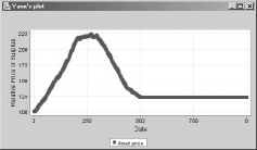
With the first model of rationality, we obtain, as expected, a very clean bubble. The simplest case, illustrated by figure 1, shows a linear and symmetric bubble that corresponds to a strictly linear risk estimation. Prices are climbing while $r(t)$ remains below 0.5 and then start to go downward as selling shares becomes more likely than buying shares. More realistic looking bubbles with a steeper crash were obtained by using an $\arctan$-based function instead of a linear one but as the behaviour observed in this case is trivially dictated by the shape of the risk function, these experiments should not get much more attention nor be seen as anything else than an empirical proof of consistence for our implementation.

Figure 1: (left) Risk is set exogenously to simulate linearly decreasing hopes for dividend collecting. (right) Corresponding numbers of buying and selling offers (center) A speculative bubble is observed wrt a fundamental value of 100

4.2 Endogenous risk

The second case is much more interesting. Market behaviour is not trivial anymore with respect to the risk estimation function and we are going to see how one can navigate between efficiency and “bubbly behaviour” by playing on the distribution of parameter values across the population.

4.2.1 Efficiency

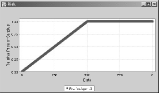
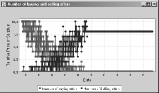
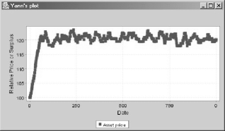
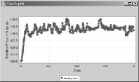
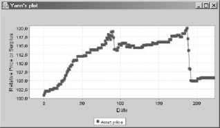
When the population of agents is initialized homogenously with the default values, the market is, as illustrated by figure 2, relatively stable as prices remain close (within a 2% or 3% range) of $F$. As illustrated by figure 3, when $F$’s value is suddenly changed, prices quickly reflect this modification. The market appears in such cases and naturally enough, as nearly efficient as it reflects stability or changes in common beliefs.

Figure 2: When there is no heterogeneity and prices are close to $F$, the market is stable: prices remain within 2 or 3 percent of F

Figure 3: The market is nearly efficient: at iteration 250, F is switched to 75 and prices quickly reflect this sudden change in common beliefs.

4.2.2 “Bubbly” behaviour

Bubbles without a crash

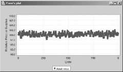
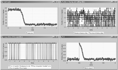
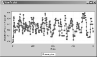
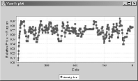
All other parameters being the same for all agents, as soon as one introduces heterogeneity in risk tolerance ($R_{0}$), which means agents are initialized with a value for $R_{0}$ that is drawn from a uniform distribution instead of being the same for everyone, speculative behaviour start to appear with prices that tend to move away from the commonly held view of $F$’s value. For instance, as shown in figure 4, with a biased upward spread for $R_{0}$ of 0.4, which means that agents have values for $R_{0}$ that lie between 0.4 and 0.8 instead of having a common default value of 0.5, we observe a rise in prices followed by a jittery oscillation.

Figure 4: A speculative bubble with no crash obtained by distributing $R_{0}$ in [0.4;0.8]

Influence of $\alpha$

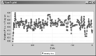
This is conditioned by the “fool factor”’s value $\alpha$. Figure 5 show that the bigger alpha is, the larger the speculation’s magnitude gets. This seems natural as increasing $\alpha$ increases the number of agents that, under similar risk conditions, keep on buying shares a large proportion of the time.

Figure 5: Different values for $\alpha$: (top left)1.0,(top right)1.05,(bottom left)1.1,(bottom right)1.2. Increasing $\alpha$ increases the magnitude of the oscillation.

Introducing asymmetry

Real speculative bubbles (i.e. price explosions followed by a steep crash) can only be obtained when, additionally to biased heterogeneity in $R_{0}$, one introduces asymmetry in the agents’ pricing strategy for the panic mode (they use $U_{[-5\%;0]}$ instead of $U_{[-1\%;+1\%]}$). A slight increase in the sensitivity to the price’s derivative ($w=-5$instead of $w=-3$) also helps to obtain full and sudden crashes. Figure 6 shows such a bubble.

Figure 6: A speculative bubble obtained with $R_{0}$ in $U_{[0.4;0.8]}$, $w=-5$ and asymmetric pricing when agents are panicking

5 Conclusion

We described a simple computational simulation of a financial asset trading environment where a community of artificial agents base their decisions to buy or sell shares on an estimation of current market risk. Two contexts were studied for this estimation: a restricted one with a finite time horizon and an exogenous risk function and a more refined one, free of any time limitation and based on a more sophisticated, although still bounded, rationality for individual agents. Within this restricted model, we experimentally derive a set of necessary and sufficient conditions for the existence of speculative phenomena, that is variations in prices that are not explainable by the asset’s underlying fundamental value, typically upward bubbles and sudden crashes. These conditions are somewhat fuzzy and correlated but clearly state the importance of heterogeneity, asymmetric behaviour and sensitivity to recent trends in the birth and rise of financial panics.

References

- [1] J. Arifovic. The behavior of the exchange rate in the genetic algorithm and experimental economies. Journal of Political Economy, 104(3):510–541, 1996.
- [2] W. B. Arthur. Inductive reasoning and bounded rationality (the el farol problem). American Econonmic Review, 84:406, 1994.
- [3] W. B. Arthur, J. Holland, B. LeBaron, R. Palmer, and P. Tayler. The Economy as an Evolving Complex System II, chapter Asset pricing under endogenous expectations in an artificial stock market, pages 15–44. Addison-Wesley, Reading, MA, 1997.
- [4] A. Beltratti and S. Margarita. From Animals to Animats 2, chapter Evolution of trading strategies among heterogeneous artificial economic agents. The MIT Press, Cambridge, MA, 1993.
- [5] J. Duffy and Utku Unver M. Asset price bubbles and crashes with near-zero-intelligence traders, towards an understanding of laboratory findings. Working paper - JEL Classification Nos. D83, D84, G12., January 2003.
- [6] S. J. Grossman and J. E. Stiglitz. On the impossibility of informationally efficient markets. The American Economic Review, 70:393–408, June 1980.
- [7] B. LeBaron. Time series properties of an artificial stock market. Journal of Economic Dynamics and Control, 23:1487–1516, 1999.
- [8] B. LeBaron. Agent based computational finance: Suggested readings and early research. Journal of Economic Dynamics and Control, 24:679–702, 2000.
- [9] B. LeBaron. A builder’s guide to agent based financial markets. Quantitative Finance, 1(2):254–261, February 2001.
- [10] B. LeBaron. Building the santa fe artificial stock market. Working Paper, Graduate School of International Economics and Finance, Brandeis University, Waltham, MA., June 2002.
- [11] C. Noussair, S. Robin, and B. Ruffieux. Price bubbles in laboratory asset markets with constant fundamental values. Experimental Economics, 4.
- [12] R. Radner. Rational expectations equilibrium: Generic existence and the information revealed by prices. Econometrica, 47(3):655–678, May 1979.
- [13] B. Ruffieux. Les marchés testés en laboratoire. Pour la science, 307:85–92, May 2003.
- [14] Y. Semet. Agent-based computational economics and finance: early research and design issues. Economic Modelling report, DREAM project, IST-1999-12679. European Community’s “Information Society Technologies” Programme (1992-2002), 2003.
- [15] Vernon L Smith, Gerry L Suchanek, and Arlington W Williams. Bubbles, crashes, and endogenous expectations in experimental spot asset markets. Econometrica, 56(5):1119–51, 1991.
- [16] L. Tesfatsion. Agent-based computational economics: Growing economies from the bottom up. Artificial Life, 8(1):55–82, 2001.