An introspective algorithm for the integer determinant

Abstract

We present an algorithm for computing the determinant of an integer matrix $A$. The algorithm is introspective in the sense that it uses several distinct algorithms that run in a concurrent manner. During the course of the algorithm partial results coming from distinct methods can be combined. Then, depending on the current running time of each method, the algorithm can emphasize a particular variant. With the use of very fast modular routines for linear algebra, our implementation is an order of magnitude faster than other existing implementations. Moreover, we prove that the expected complexity of our algorithm is only $O\big{(}n^{3}\log^{2.5}\left(n\|A\|\right)\big{)}$ bit operations in the case of random dense matrices, where $n$ is the dimension and $\|A\|$ is the largest entry in the absolute value of the matrix.

1 Introduction

One has many alternatives to compute the determinant of an integer matrix. Over a field, the computation of the determinant is tied to that of matrix multiplication via block recursive matrix factorizations [19]. On the one hand, over the integers, a naïve approach would induce a coefficient growth that would render the algorithm not even polynomial. On the other hand, over finite fields, one can nowadays reach the speed of numerical routines [12].

Therefore, the classical approach over the integers is to reduce the computation modulo some primes of constant size and to recover the integer determinant from the modular computations. For this, at least two variants are possible: Chinese remaindering and $p$-adic lifting.

The first variant requires either a good a priori bound on the size of the determinant or an early termination probabilistic argument [13, §4.2]. It thus achieves an output dependant bit complexity of $O\big{(}\log\left(|\det\left(A\right)|\right)\left(n^{\omega}+n^{2}\log\left(\|A\|\right)\right)\big{)}$ where $\omega$ is the exponent of matrix multiplication . Of course, with the coefficient growth, the determinant size can be as large as $O\left(n\log(n\|A\|)\right)$ (Hadamard’s bound) thus giving a large worst case complexity. The algorithm is Monte Carlo type, its deterministic (always correct) version exists and has the complexity of $O\left(\left(n^{\omega+1}+n^{3}\log(\|A\|)\right)\log(n\|A\|)\right)$ bit operations.

The second variant uses system solving and $p$-adic lifting [6] to get a potentially large factor of the determinant with a $O\left(n^{3}\log^{2}(n\|A\|)\right)$ bit complexity. Indeed, every integer matrix is unimodularly equivalent to a diagonal matrix $S$ equal to $\operatorname{diag}\left(s_{1},\dots,s_{n}\right)$, where $s_{i}$ divides $s_{i+1}$. This means that there exist integer matrices $U,V$ with $\det{U},\det{V}=\pm 1$, such that $A=USV$. The $s_{i}$ are called the invariant factors of A. In the presence of several matrices we will also use the notation $s_{i}(A)$. Solving a linear system with a random right hand side reveals $s_{n}$ as the common denominator of the solution vector entries with high probability, see [24, 1].

The idea of [1] is thus to combine both approaches, i.e. to approximate the determinant by system solving and recover only the remaining part ($\det(A)/s_{n}$) via Chinese remaindering. The Monte Carlo version of Chinese remaindering leads to an algorithm with the expected output-dependant bit complexity of $O\big{(}n^{\omega}\log\left(|\frac{\det(A)}{s_{n}}|\right)+n^{3}\log^{2}(n\|A\|)\big{)}$. We use the notion of the expected complexity to emphasize that it requires $\mathbf{E}\left(log\left(\frac{s_{n}}{\tilde{s}_{n}}\right)\right)$ to be $O(1)$, where $\tilde{s}_{n}$ is the computed factor of $s_{n}$ and $\mathbf{E}$ denotes the expected value computed over all algorithm instances for a given matrix $A$.

Then G. Villard remarked that at most $O\left(\sqrt{\log\left(|\det\left(A\right)|\right)}\right)$ invariant factors can be distinct and that in some propitious cases we can expect that only the last $O\left(\log(n)\right)$ of those are nontrivial [17]. This remark, together with a preconditioned $p$-adic solving to compute the $i$-th invariant factor lead to a $O\left(n^{2+\frac{\omega}{2}}\log^{1.5}(n\|A\|)\log^{0.5}(n)\right)$ worst case Monte Carlo algorithm. Without fast matrix multiplication, the complexity of the algorithm becomes $O\left(n^{3.5}\log^{2.5}(n\|A\|)\log^{2}(n)\right)$. The expected number of invariant factors for a set of matrices with entries chosen randomly and uniformly from the set of consecutive integers $\{0,1\dots\dots\lambda-1\}$ can be proven to be $O\left(\log(n)\right)$. Thus, we can say that the expected complexity of the algorithm is $O\left(n^{3}\log^{2}(n\|A\|)\log(n)\log_{\lambda}(n)\right)$. Here, the term expected is used in a slightly different context than in algorithm [1] and describes the complexity in the case where the matrix has a propitious property i.e., the small number of invariant factors.

In this paper we will prefer to use the notion of the expected rather than average complexity. Formally, to compute the average complexity we have to average the running time of the algorithm over all input and argorithm instances. The common approach is thus to compute the expected outputs of the subroutines and use them in the complexity analysis. This allows us to deal easily with complex algorithms with many calls to subroutines which depend on randomization. The two approaches are equivalent when the dependency on the expected value is linear, which is often the case. However, we can imagine more complex cases of adaptive algorithms where the relation between average and expected complexity is not obvious. Nevertheless, we believe that the evaluation of the expected complexity gives a meaningful description of the algorithm. We emphasize the fact, that the propitious input for which the analysis is valid can often be quickly detected at runtime.

Note that the actual best worst case complexity algorithm for dense matrices is $O^{\sim}\left(n^{2.7}\log(\|A\|)\right)$, which is $O^{\sim}\left(n^{3.2}\log(\|A\|)\right)$ without fast matrix multiplication, by [21]. We use the notion $O^{\sim}(N^{\alpha}\log(\|A\|))$, which is equivalent to $O(N^{\alpha}\log^{\beta}(N)\log(\|A\|))$ with some $\beta\geq 0$. Unfortunately, these last two worst case complexity algorithms, though asymptotically better than [17], are not the fastest for the generic case or for the actually attainable matrix sizes. The best expected complexity algorithm is the Las Vegas algorithm of Storjohann [26] which uses an expected number of $O\left(n^{\omega}\log(n\|A\|)\log^{2}(n)\right)$ bit operations. In section 5 we compare the performance of this algorithm (for both certified and not certified variants) to ours, based on the experimental results of [27].

In this paper, we propose a new way to extend the idea of [25, 28] to get the last consecutive invariant factors with high probability in section 3.2. Then we combine this with the scheme of [1].

This combination is made in an adaptive way. This means that the algorithm will choose the adequate variant at run-time, depending on discovered properties of its input. More precisely, in section 4, we propose an algorithm which uses timings of its first part to choose the best termination. This particular kind of adaptation was introduced in [23] as introspective; here we use the more specific definition of [5].

In section 4.2 we prove that the expected complexity of our algorithm is

$$O\left(n^{3}\log^{2}(n\|A\|)\sqrt{\log(n)}\right)$$

bit operations in the case of dense matrices, gaining a $\log^{1.5}(n)$ factor compared to [17].

Moreover, we are able to detect the worst cases during the course of the algorithm and switch to the asymptotically fastest method. In general this last switch is not required and we show in section 5 that when used with the very fast modular routines of [9, 12] and the LinBox library [10], our algorithm can be an order of magnitude faster than other existing implementations.

A preliminary version of this paper was presented in the Transgressive Computing 2006 conference [14]. Here we give better asymptotic results for the dense case, adapt our algorithm to the sparse case and give more experimental evidences.

2 Base Algorithms and Procedures

In this section we present the procedures in more detail and describe their probabilistic behavior. We start by a brief description of the properties of the Chinese Remaindering loop (CRA) with early termination (ET) (see [7]), then proceed with the LargestInvariantFactor algorithm to compute $s_{n}$ (see [1, 17, 25]). We end the section with a summary of ideas of Abbott et al. [1], Eberly et al. and Saunders et al. [25].

2.1 Output dependant Chinese Remaindering Loop (CRA)

CRA is a procedure based on the Chinese remainder theorem. Determinants are computed modulo several primes $p_{i}$. Then the determinant is reconstructed modulo $p_{0}\cdots p_{t}$ in the symmetric range via the Chinese reconstruction. The integer value of the determinant is thus computed as soon as the product of $p_{i}$ exceeds $2|\det\left(A\right)|$. We know that the product is sufficiently big if it exceeds some upper bound on this value or, probabilistically, if the reconstructed value remains identical for several successive additions of modular determinants. The principle of this early termination (ET) is thus to stop the reconstruction before reaching the upper bound, as soon as the determinant remains the same for several steps [7].

Algorithm 1 is an outline of a procedure to compute the determinant using CRA loops with early termination, correctly with probability $1-\epsilon$. We start with a lemma.

Lemma 2.1.

Let $H$ be an upper bound for the determinant (e.g. $H$ can be the Hadamard’s bound: $|det\left(A\right)|\leq\left(\sqrt{n}\|A\|\right)^{n}$). Suppose that distinct primes $p_{i}$ greater than $l>0$ are randomly sampled from a set $P$ with $|P|\geq 2\lceil\log_{l}\left(H\right)\rceil$. Let $r_{t}$ be the value of the determinant modulo $p_{0}\cdots p_{t}$ computed in the symmetric range. We have:

1. $r_{t}=\det\left(A\right)$, if $t\geq N=\begin{cases}\lceil\log_{l}\left(|\det\left(A\right)|\right)\rceil&\text{if}~{}\det\left(A\right)\neq 0\\ 0&\text{if}~{}\det\left(A\right)=0\end{cases}$;

2. if $r_{t}\neq\det\left(A\right)$, then there are at most $R=\lceil\log_{l}\left(\frac{|\det\left(A\right)-r_{t}|}{p_{0}\cdots p_{t}}\right)\rceil$ primes $p_{t+1}$ such that $r_{t}=\det\left(A\right)$ mod $p_{0}\cdots p_{t}p_{t+1}$;

3. if $r_{t}=r_{t+1}=\cdots=r_{t+k}$ and $\frac{R^{\prime}\left(R^{\prime}-1\right)\dots\left(R^{\prime}-k+1\right)}{\left(|P|-t-1\right)\dots\left(|P|-t-k\right)}<\epsilon$, where $R^{\prime}=\lceil\log_{l}\frac{H+|r_{t}|}{p_{0}p_{1}\dots p_{t}}\rceil$, then $\mathcal{P}\left(r_{t}\neq\det\left(A\right)\right)<\epsilon$.

4. if $r_{t}=r_{t+1}=\cdots=r_{t+k}$ and $k\geq\lceil\frac{\log\left(1/\epsilon\right)}{\log\left(P^{\prime}\right)-\log\left(\log_{l}\left(H\right)\right)}\rceil$, where $P^{\prime}=|P|-\lceil\log_{l}\left(H\right)\rceil$, then $\mathcal{P}\left(r_{t}\neq\det\left(A\right)\right)<\epsilon$.

Proof.

For (i), notice that $-\lfloor\frac{p_{0}\cdots p_{t}}{2}\rfloor\leq r_{t}<\lceil\frac{p_{0}\cdots p_{t}}{2}\rceil$. Then $r_{t}=\det\left(A\right)$ as soon as $p_{0}\cdots p_{t}\geq 2|\det\left(A\right)|$. With $l$ being the lower bound for $p_{i}$ this reduces to $t\geq\lceil\log_{l}{|\det\left(A\right)|}\rceil$ when $\det\left(A\right)\neq 0$.
For (ii), we observe that $\det\left(A\right)=r_{t}+Kp_{0}\dots p_{t}$ and it suffices to estimate the number of primes greater than $l$ dividing $K$.
For (iii) we notice that $k$ primes dividing $K$ are to be chosen with the probability $\frac{{R\choose k}}{{{|P|-(t+1)}\choose k}}$. Applying the bound $R^{\prime}$ for $R$ leads to the result.
For (iv) we notice that the latter is bounded by $\left(\frac{R^{\prime}}{P^{\prime}}\right)^{k}$ since $R^{\prime}\leq\lceil\log_{l}\left(\frac{2H}{2}\right)\rceil\leq|P^{\prime}|$. Solving for $k$ the inequality $\left(\frac{R^{\prime}}{P^{\prime}}\right)^{k}<\epsilon$ gives the result. ∎

The two last points of the theorem give the stopping condition for early termination. The condition (iii) can be computed on-the-fly (as in Algorithm 1). As a default value and for simplicity (iv) can also be used.

Algorithm 1 Early Terminated CRA

0:  $n\times n$ integer matrix $A$.

0:  $0<\epsilon<1$.

0:  $H$ - Hadamard’s bound ($H=\left(\sqrt{n}\|A\|\right)^{n}$)

0:  $l>0$, a set P of random primes greater than $l$, $|P|\geq 2\lceil\log_{l}\left(H\right)\rceil$.

0:  The integer determinant of $A$, correct with probability at least $1-\epsilon$.

1:  $i=0$;

2:  repeat

3:     Choose uniformly and randomly a prime $p_{i}$ from the set $P$;

4:     $P=P\backslash\{p_{i}\}$

5:      Compute $\det\left(A\right)$ mod $p_{i}$;

6:     Reconstruct $r_{i}$, the determinant modulo $p_{0}\cdots p_{i}$; // by Chinese remaindering

7:     $k=\max\{t:r_{i-t}=\dots=r_{i}\}$; $R^{\prime}=\lceil\log_{l}\frac{H+|r_{i}|}{p_{0}p_{1}\dots p_{i-k}}\rceil$;

8:     Increment i;

9:  until $\frac{R^{\prime}\left(R^{\prime}-1\right)\dots\left(R^{\prime}-k+1\right)}{\left(|P|-i+k-1\right)\dots\left(|P|-i\right)}<\epsilon$ or $\prod p_{i}\geq 2H$

To compute the modular determinant in algorithm 5 we use the LU factorization modulo $p_{i}$. Its complexity is $O\left(n^{\omega}+n^{2}\log(\|A\|)\right)$.

Early termination is particularly useful in the case when the computed determinant is much smaller than the a priori bound. The running time of this procedure is output dependant.

2.2 Largest Invariant Factor

A method to compute $s_{n}$ for integer matrices was first stated by V. Pan [24] and later in the form of the LargestInvariantFactor procedure (LIF) in [1, 17, 7, 25]. The idea is to obtain a divisor of $s_{n}$ by computing a rational solution of the linear systems $Ax=b$. If $b$ is chosen uniformly and randomly from a sufficiently large set of contiguous integers, then the computed divisor can be as close as possible to $s_{n}$ with high probability. Indeed, with $A=USV$, we can equivalently solve $SVx=U^{-1}b$ for $y=Vx$, and then solve for $x$. As $U$ and $V$ are unimodular, the least common multiple of the denominators of $x$ and $y$, $d(x)$ and $d(y)$ satisfies $d(x)=d(y)\arrowvert s_{n}$.

Thus, solving $Ax=b$ enables us to get $s_{n}$ with high probability. The cost of solving using Dixon $p$-adic lifting [6] is $O\left(n^{3}\log^{2}(n\|A\|)+n\log^{2}(\|b\|)\right)$ as stated by [22].

The algorithm takes as input parameters $\beta$ and $r$ which are used to control the probability of correctness; $r$ is the number of successive solvings and $\beta$ is the size of the set from which the values of a random vector $b$ are chosen, i.e. a bound for $\|b\|$. With each system solving, the output $\tilde{s}_{n}$ of the algorithm is updated as the $\operatorname{lcm}$ of the current solution denominator $d(x)$ and the result obtained so far.

The following theorem characterizes the probabilistic behavior of the LIF procedure.

Theorem 2.2.

Let $A$ be a $n\times n$ matrix, $H$ its Hadamard’s bound, $r$ and $\beta$ be defined as above. Then the output $\tilde{s}_{n}$ of Algorithm LargestInvariantFactor of [1] is characterized by the following properties.

1. If $r=1$, $p$ is a prime, $l\geq 1$, then $\mathcal{P}\left(p^{l}\arrowvert\frac{s_{n}}{\tilde{s}_{n}}\right)\leq\frac{1}{\beta}\lceil\frac{\beta}{p^{l}}\rceil;$

2. if $r=2$, $\beta=\lceil\log\left(H\right)\rceil$ then $\mathbf{E}\left(\log\left(\frac{s_{n}}{\tilde{s}_{n}}\right)\right)=O\left(1\right);$

3. if $r=2$, $\beta=6+\lceil 2\log\left(H\right)\rceil$ then $s_{n}=\tilde{s}_{n}$ with probability at least 1/3;

4. if $r=\lceil 2\log\left(\log\left(H\right)\right)\rceil$, $\beta\geq 2$ then $\mathbf{E}\left(\log\left(\frac{s_{n}}{\tilde{s}_{n}}\right)\right)=O\left(1\right);$

5. if $r=\lceil\log\left(\log\left(H\right)\right)+\log\left(\frac{1}{\epsilon}\right)\rceil$, $2\mid\beta$ and $\beta\geq 2$ then $s_{n}=\tilde{s}_{n}$ with probability at least $1-\epsilon$;

Proof.

The proofs of (i) and (iv) are in [1][Thm. 2, Lem. 2]. The proof of (iii) is in [17][Thm. 2.1]. To prove (ii) we adapt the proof of (iii). The expected value of the under-approximation of $s_{n}$ is bounded by the formula

$$\sum_{p\mid s_{n}}\sum_{k=1}^{\lfloor\log_{p}\left(s_{n}\right)\rfloor}\log\left(p\right)\left(\frac{1}{\beta}\lceil\frac{\beta}{p^{k}}\rceil\right)^{2},$$

where the sum is taken over all primes dividing $s_{n}$. As $\frac{1}{\beta}\lceil\frac{\beta}{p^{k}}\rceil$ is bounded by $\frac{1}{\beta}+\frac{1}{p^{k}}$ this can be further expressed as

$$\sum_{p~{}prime}\sum_{k=1}^{\infty}\log\left(p\right)\frac{1}{p^{2k}}+\frac{2}{\beta}\sum_{p\mid s_{n}}\sum_{k=1}^{\infty}\log\left(p\right)\frac{1}{p^{k}}+\frac{1}{\beta^{2}}\sum_{p\mid s_{n}}\sum_{k=1}^{\lfloor\log_{p}\left(s_{n}\right)\rfloor}\log\left(p\right)\leq$$

$$\sum_{p~{}prime}\log\left(p\right)\frac{1}{p^{2}-1}+\frac{2}{\beta}\sum_{p\mid s_{n}}\log\left(p\right)\frac{1}{p-1}+\frac{1}{\beta^{2}}\sum_{p\mid s_{n}}\log\left(p\right)\log_{p}\left(s_{n}\right)$$

$$1.78+\frac{2\log\left(s_{n}\right)}{\beta}+\frac{\log^{2}\left(s_{n}\right)}{\beta^{2}}\leq 5\in O\left(1\right).$$

To prove (v) we slightly modify the proof of (iv) in the following manner. From (i) we notice that for every prime $p$ dividing $s_{n}$, the probability that it divides the missed part of $s_{n}$ satisfies:

$$\mathcal{P}\left(p\mid\frac{s_{n}}{\tilde{s}_{n}}\right)\leq\left(\frac{1}{2}\right)^{r}.$$

As there are at most $\log\left(H\right)$ such primes, we get

$$\mathcal{P}\left(s_{n}=\tilde{s}_{n}\right)\geq 1-\log\left(H\right)\left(1/2\right)^{r}\geq 1-\log\left(H\right)2^{-\log\left(\log\left(H\right)\right)-\log\left(\frac{1}{\epsilon}\right)}=1-\log\left(H\right)\frac{1}{\log\left(H\right)}\epsilon.$$

∎

Remark 2.3.

Theorem 2.2 enables us to produce a LIF procedure, which gives an output $\tilde{s}$ close to $s_{n}$ with the time complexity $O\left(n^{3}\left(\log\left(n\right)+\log\left(\|A\|\right)\right)^{2}\right)$ (see (ii)).

2.3 Abbott-Bronstein-Mulders, Saunders-Wan and Eberly-Giesbrecht-Villard ideas

Now, the idea of [1] is to combine both the Chinese remainder and the LIF approach. Indeed, one can first compute $s_{n}$ and then reconstruct only the remaining factors of the determinant by reconstructing $\det\left(A\right)/s_{n}$. The expected complexity of this algorithm is $O\left(n^{\omega}\log\left(|\det(A)/s_{n}|\right)+n^{3}\log^{2}(n\|A\|)\right)$ which is unfortunately $O^{\sim}\left(n^{\omega+1}\right)$ in the worst case.

Now Saunders and Wan [25, 28] proposed a way to compute not only $s_{n}$ but also $s_{n-1}$ (which they call a bonus) in order to reduce the size of the remaining factors $\det(A)/\left(s_{n}s_{n-1}\right)$. The complexity doesn’t change.

Then, Eberly, Giesbrecht and Villard have shown that for the dense case the expected number of non trivial invariant factors is small, namely less than $3\lceil\log_{\lambda}\left(n\right)\rceil+29$ if the entries of the matrix are chosen uniformly and randomly in a set of $\lambda$ consecutive integers [17]. As they also give a way to compute any $s_{i}$, this leads to an algorithm with the expected complexity $O\left(n^{3}\log^{2}(n\|A\|)\log\left(n\right)\log_{\lambda}\left(n\right)\right)$.

Our analysis yields that the bound on the expected number of invariant factors for

a random dense matrix can be refined as $O\left(\log^{0.5}\left(n\right)\right)$.

Then our idea is to extend the method of Saunders and Wan to get the last invariant factors of $A$ slightly faster than by [17]. Moreover, we will show in the following sections that we are able to build an adaptive algorithm solving a minimal number of systems.

The analysis also yields that it should be possible to change a $\log\left(n\right)$ factor in the expected complexity of [17] to a $\log(\log\left(n\right))$. This would require a small modification in the algorithm and a careful analysis. Assuming that the number of invariant factors is the expected i.e. it equals $N=O\left(\log\left(n\right)\right)$, we can verify the hypothesis by computing the $(n-N-1)$th factor. If it is trivial, the binary search is done among $O\left(\log\left(n\right)\right)$ elements and there are only $O\left(\log\left(n\right)\right)$ factors to compute, which allows to lessen the probability of correctness of each OIF procedure. Thus, in the propitious case, the expected complexity of the algorithm would be $O\left(n^{3}\log^{2}(n\|A\|)\log_{\lambda}\left(n\right)\log^{2}(\log(n))\right)$. However, this cannot ce considered as the average complexity in the ordinary sense since we do not average over all possible inputs in the analysis.

3 Computing the product of $O\left(\log(n)\right)$ last invariant factors

3.1 On the number of invariant factors

The result in [17] says that a $n\times n$ matrix with entries chosen randomly and uniformly from a set of size $\lambda$ has the expected number of invariant factors bounded by $3\lceil\log_{\lambda}\left(n\right)\rceil+29$. In search for some sharpening of this result we prove the following theorems.

Theorem 3.1.

Let $A$ be an $n\times n$ matrix with entries chosen randomly and uniformly from the set of contiguous integers $\{-\lfloor\frac{\lambda}{2}\rfloor\dots\lceil\frac{\lambda}{2}\rceil\}$. Let $p$ be a prime. The expected number of non-trivial invariant factors of $A$ divisible by $p$ is at most 4.

Theorem 3.2.

Let $A$ be an $n\times n$ matrix with entries chosen randomly and uniformly from the set $\{-\lfloor\frac{\lambda}{2}\rfloor\dots\lceil\frac{\lambda}{2}\rceil\}$. The expected number of non trivial invariant factors of $A$ is at most $\left\lceil\sqrt{2\log_{\lambda}\left(n\right)}\right\rceil+3$.

In order to prove the theorems stated above, we start with the following lemmas.

Lemma 3.3.

If $j>$1 the sum $\displaystyle\sum_{8<p<\lambda}\left(\frac{1}{\lambda}\lceil\frac{\lambda}{p}\rceil\right)^{j}$ over primes $p$ can be upper bounded by $\left(\frac{1}{2}\right)^{j}$.

Proof.

We will consider separately the primes from the interval $\frac{\lambda}{2^{k+1}}\leq p<\frac{\lambda}{2^{k}}$, $k=0,1,\dots k_{max}$. The value of $k_{max}$ is computed from the condition $p>8$ and is equal to $\lceil\log\left(\lambda\right)\rceil-4$. For the $k$th interval $\lceil\frac{\lambda}{p}\rceil$ is less than or equal to $2^{k+1}$. In each interval there are at most $\lceil\frac{\lambda}{2^{k+2}}\rceil$ odd numbers and at most $\frac{\lambda}{2^{k+2}}$ primes: if in the interval there are more than 3 odd numbers, at least one of them is divisible by $3$ and is therefore composite. For this to happen it is enough that $\lceil\frac{\lambda}{2^{k_{max}+2}}\rceil\geq 3$, which is the case. We may therefore calculate:

$$\sum_{8<p<\lambda}\left(\frac{1}{\lambda}\lceil\frac{\lambda}{p}\rceil\right)^{j}\leq\sum_{k=0}^{\lceil\log\left(\lambda\right)\rceil-4}\frac{\lambda}{2^{k+2}}\left(\frac{2^{k+1}}{\lambda}\right)^{j}\leq\sum_{k=0}^{\lceil\log\left(\lambda\right)\rceil-4}\frac{1}{2}\left(\frac{2^{k+1}}{\lambda}\right)^{j-1}=\frac{1}{2\lambda^{j-1}}\sum_{k=0}^{\lceil\log\left(\lambda\right)\rceil-4}\left(2^{k+1}\right)^{j-1}$$

$$\leq\frac{1}{2\lambda^{j-1}}\left(\sum_{k=0}^{\lceil\log\left(\lambda\right)\rceil-4}2^{k+1}\right)^{j-1}\leq\frac{1}{2\lambda^{j-1}}\left(2^{\lceil\log\left(\lambda\right)\rceil-2}\right)^{j-1}\leq\frac{1}{2\lambda^{j-1}}\left(2^{\log\left(\lambda\right)-1}\right)^{j-1}=\left(\frac{1}{2}\right)^{j}.$$

∎

Remark 3.4.

For $\lambda=2^{l}$, $k$ can be allowed from $0$ up to $l-3$, instead of $\lceil\log\left(\lambda\right)\rceil-4$ and we can include more primes in the sum. As a result we obtain an inequality $\sum_{4<p<2^{l}}\left(\frac{1}{2^{l}}\lceil\frac{2^{l}}{p}\rceil\right)^{j}\leq\left(\frac{1}{2}\right)^{j}$.

Lemma 3.5.

Let $A$ be a $k\times n$, $k\leq n$ integer matrix with entries chosen uniformly and randomly from the set $\{-\lfloor\frac{\lambda}{2}\rfloor\dots\lceil\frac{\lambda}{2}\rceil\}$ . The probability that $\operatorname{rank}_{p}(A)$, the rank modulo $p$ of $A$, is $j$, $0<j\leq k$ is less than or equal to

$$\mathcal{P}\left(\operatorname{rank}_{p}(A)=j\right) \leq\prod_{i=0}^{j-1}(1-\alpha^{(n-i)})\cdot\beta^{(n-j)(k-j)}\cdot\left(\frac{1}{1-\beta}\right)^{\max{k-j-1,0}}(1+\beta\dots\beta^{k-j})$$

$$\leq\beta^{(n-j)(k-j)}\left(\frac{1}{1-\beta}\right)^{k-j},$$ (1)

where $\alpha=\frac{1}{\lambda+1}\lfloor\frac{\lambda+1}{p}\rfloor$ and $\beta=\frac{1}{\lambda+1}\lfloor\frac{\lambda+1}{p}\rfloor$.

The proof of the lemma is given in the appendix A.1.

Proof.

(Theorem 3.1)
The idea of the proof is similar to that of [17][Thm. 6.2].

For $k\geq j$ let $\operatorname{MDep}_{k}\left(p,j\right)$ denote the event that the first $k$ columns of $A$ mod $p$ have rank at most $k-j$ over $\mathbb{Z}_{p}$. By $I_{j}\left(p\right)$ we denote the event, that at least $j$ invariant factors of $A$ are divisible by $p$. This implies that the first columns of $A$ have rank at most $n-j$ mod $p$, or that $\operatorname{MDep}_{n-j+k}\left(p,k\right)$ has occurred for all $k=0\dots j$. This proves in particular that $\mathcal{P}\left(I_{j}\left(p\right)\right)\leq\mathcal{P}\left(\operatorname{MDep}_{n}\left(p,j\right)\right)$.

In order to compute the probability $\mathcal{P}\left(\operatorname{MDep}_{s}\left(p,j\right)\right)$, $s\geq j$ we notice that it is less than or equal to

$$\mathcal{P}\left(\operatorname{MDep}_{s}\left(p,j\right)\right)\leq\mathcal{P}\left(\operatorname{MDep}_{j}\left(p,j\right)\right)+\sum_{k=j+1}^{s}\mathcal{P}\left(\operatorname{MDep}_{k}\left(p,j\right)\wedge\neg\operatorname{MDep}_{k-1}\left(p,j\right)\right)$$

Surely, $\operatorname{MDep}_{j}\left(p,j\right)$ means that the first $j$ columns of $A$ are 0 mod $p$, and consequently the probability is less than or equal to $\beta_{p}^{jn}$, where the value $\beta_{p}=\frac{1}{\lambda+1}\lceil\frac{\lambda+1}{p}\rceil$ is a bound on the probability that an entry of the matrix is determined modulo $p$ and is set to $(\lambda+1)^{-1}$ if $p\geq\lambda+1$ or less than or equal $\frac{2}{p+1}$ in the case $p<\lambda+1$.

We are now going to find $\mathcal{P}\left(\operatorname{MDep}_{k}\left(p,j\right)\wedge\neg\operatorname{MDep}_{k-1}\left(p,j\right)\right)$ for $k>j$. Since the event $\operatorname{MDep}_{k-1}\left(p,j\right)$ did not occur, $A_{k-1}$ has rank modulo $p$ at least $\left(k-j\right)$ and of course at most $\left(k-1\right)$. For $\operatorname{MDep}_{k,j}$ to occur it must be exactly $\left(k-j\right)$. This means that we can rewrite $\mathcal{P}\left(\operatorname{MDep}_{k}\left(p,j\right)\wedge\neg\operatorname{MDep}_{k-1}\left(p,j\right)\right)$ as

$$\mathcal{P}\left(\operatorname{MDep}_{k}\left(p,j\right)\mid\operatorname{rank}_{p}\left(A_{k-1}\right)=k-j\right)\cdot\mathcal{P}\left(\operatorname{rank}_{p}\left(A_{k-1}\right)=k-j\right),$$

where $\operatorname{rank}_{p}\left(A_{k-1}\right)$ denotes the rank modulo $p$ of submatrix $A_{k-1}$ of $A$, which consists of its first $\left(k-1\right)$ columns.

Since the rank modulo $p$ of $A_{k-1}$ is equal to $k-j$, there exists a set of $k-j$ rows $L_{k-j}$ which has full rank mod p. This means that we can choose $k-j$ entries of the $k$th column randomly but the remaining $n-k+j$ entries will be determined modulo $p$. This leads to an inequality

$$\mathcal{P}\left(\operatorname{MDep}_{k}\left(p,j\right)~{}|~{}\operatorname{rank}_{p}\left(A_{k-1}\right)=k-j\right)\leq\beta_{p}^{n-k+j}.$$

By Lemma 3.5 we have $\mathcal{P}(\operatorname{rank}(A_{k-1}=k-j)\leq\left(\frac{1}{1-\beta_{p}}\right)^{j-1}\beta_{p}^{(n-k+j)(j-1)}$. Finally, we get

$$\mathcal{P}\left(\operatorname{MDep}_{k}\left(p,j\right)\wedge\neg\operatorname{MDep}_{k-1}\left(p,j\right)\right)\leq\left(\frac{1}{1-\beta_{p}}\right)^{j-1}\beta_{p}^{(n-k+j)j}$$ (2)

and

$$\mathcal{P}\left(\operatorname{MDep}_{s}\left(p,j\right)\right)\leq\left(\frac{1}{1-\beta_{p}}\right)^{j-1}\sum_{k=j}^{s}\beta_{p}^{\left(n-k+j\right)j}<\left(\frac{1}{1-\beta_{p}}\right)^{j-1}\beta_{p}^{j(n-s+j)}\frac{1}{1-\beta_{p}^{j}}.$$ (3)

The expected number of invariant factor divisible by $p<\lambda$ verifies:

$$\sum_{j=0}^{n}j\left(P\left(I_{j}\left(p\right)\right)-P\left(I_{j+1}\left(p\right)\right)\right) =\sum_{j=1}^{n}P\left(I_{j}\left(p\right)\right)\leq\sum_{j=1}^{n}\operatorname{MDep}_{n}\left(p,j\right)$$

$$\leq\sum_{j=1}^{n}\left(\frac{p+1}{p-1}\right)^{j-1}\left(\frac{2}{p+1}\right)^{j^{2}}\frac{\left(p+1\right)^{j}}{\left(p+1\right)^{j}-2^{j}}$$

The latter is decreasing in $p$ and therefore less than its value at $p=2$, which is lower than 3.46.

For $p\geq\lambda+1$ the result is even sharper:

$$\sum_{j=0}^{n}j\left(P\left(I_{j}\left(p\right)\right)-P\left(I_{j+1}\left(p\right)\right)\right)\leq\sum_{j=1}^{n}\left(\frac{\lambda}{\lambda-1}\right)^{j-1}\left(\frac{1}{\lambda}\right)^{j^{2}}\frac{\lambda^{j}}{\lambda^{j}-1}\leq\frac{1}{\lambda-1}\frac{1}{1-\frac{1}{(\lambda-1)\lambda^{2}}}$$

the latter being lower than 1.18 for $\lambda\geq 1$. ∎

Proof.

(Theorem 3.2)

In addition to $\operatorname{MDep}_{k}\left(p,j\right)$ introduced earlier, let $\operatorname{Dep}_{k}$ denote an event that the first $k$ columns of $A$ are linearly dependent (over rationals) and $\operatorname{MDep}_{k}\left(j\right)$, an event that either of $\operatorname{MDep}_{k}\left(p,j\right)$ occurred.

Recall from [17, §6] that

$$\mathcal{P}(\operatorname{Dep}_{1})\leq(\lambda+1)^{-n}$$

$$\mathcal{P}\left(\operatorname{Dep}_{k}\wedge\neg\operatorname{Dep}_{k-1}\right)\leq\mathcal{P}\left(\operatorname{Dep}_{k}\mid\neg\operatorname{Dep}_{k-1}\right)\leq(\lambda+1)^{-n+k-1}.$$

This gives $\mathcal{P}(\operatorname{Dep}_{k})\leq\frac{1}{(\lambda+1)^{n}}+\dots+\frac{1}{(\lambda+1)^{n-k+1}}$ which is less than $\frac{1}{(\lambda+1)^{n-k+1}}\frac{\lambda+1}{\lambda}$.

As in the previous proof, the probability that the number of non trivial invariant factors is at least $j$ (event $I_{j}$) is lower than $\mathcal{P}\left(\operatorname{MDep}_{n-j+k}(k)\vee\operatorname{Dep}_{n-j+1}\right)$ for all $k=0\dots j$. The latter can be transformed to $\mathcal{P}\left((\operatorname{MDep}_{n-j+k}(k)\wedge\neg\operatorname{Dep}_{n-j+1})\vee\operatorname{Dep}_{n-j+1}\right)$, and both $\mathcal{P}\left(\operatorname{MDep}_{n-j+k}(k)\wedge\neg\operatorname{Dep}_{n-j+1}\right)$ and $\mathcal{P}\left(\operatorname{Dep}_{n-j+1}\right)$ can be treated separately.

To compute $\mathcal{P}\left(\operatorname{MDep}_{n-j+k}(k)\wedge\neg\operatorname{Dep}_{n-j+1}\right)$ we will sum $\mathcal{P}\left(\operatorname{MDep}_{n-j+k}(p,k)\right)$ over all possible primes. Since $\operatorname{Dep}_{n-j+1}$ does not hold, there exists a $(n-j+1)\times(n-j+1)$ non-zero minor, and we have to sum over the primes which divide it. We will treat separately primes $p<\lambda+1$ and $p\geq\lambda+1$. Once again we set $\beta_{p}=\frac{2}{p+1}$ for $p<\lambda+1$ and $\beta_{p}=\frac{1}{\lambda+1}$ for $p\geq\lambda$.

By (3) we have

$$\sum_{p<\lambda}\mathcal{P}(\operatorname{MDep}_{n-j+k}(p,k))<\left(\frac{1}{1-\beta_{2}}\right)^{k-1}\beta_{2}^{kj}\frac{1}{1-\beta_{2}^{k}}+\left(\frac{1}{1-\beta_{3}}\right)^{k-1}\beta_{3}^{kj}\frac{1}{1-\beta_{3}^{k}}$$

$$+ \left(\frac{1}{1-\beta_{5}}\right)^{k-1}\beta_{5}^{kj}\frac{1}{1-\beta_{5}^{k}}+\left(\frac{1}{1-\beta_{7}}\right)^{k-1}\beta_{7}^{kj}\frac{1}{1-\beta_{7}^{k}}+\sum_{8<p<\lambda}\left(\frac{1}{1-\beta_{p}}\right)^{k-1}\beta_{p}^{kj)}\frac{1}{1-\beta_{p}^{k}}.$$

This transforms to

$$\sum_{p<\lambda}\mathcal{P}(\operatorname{MDep}_{n-j+k}(p,k))\leq 3^{k-1}\left(\frac{2}{3}\right)^{kj}\frac{3^{k}}{3^{k}-2^{k}}+2^{k-1}\left(\frac{1}{2}\right)^{kj}\frac{2^{k}}{2^{k}-1}$$

$$+ \left(\frac{3}{2}\right)^{k-1}\left(\frac{1}{3}\right)^{kj}\frac{3^{k}}{3^{k}-1}+\left(\frac{4}{3}\right)^{k-1}\left(\frac{1}{4}\right)^{kj}\frac{4^{k}}{4^{k}-1}$$

$$+\left(\frac{6}{5}\right)^{k-1}\frac{6^{k}}{6^{k}-1}\sum_{8<p<\lambda+1}\left(\frac{1}{\lambda+1}\lceil\frac{\lambda+1}{p}\rceil\right)^{kj}.$$

Thanks to Lemma 3.3, the sum $\sum_{8<p<\lambda+1}\left(\frac{1}{\lambda+1}\lceil\frac{\lambda+1}{p}\rceil\right)^{kj}$ can be bounded by $\left(\frac{1}{2}\right)^{kj}$.

For primes $p\geq\lambda+1$ we should estimate the number of primes dividing the $(n-j+1)$th minor. By the Hadamard’s bound (notice that $\operatorname{Dep}_{n-j+1}$ does not hold), the minors are bounded in absolute value by $\left(\left(n-j+1\right)\left(\frac{\lambda+1}{2})\right)^{2}\right)^{\frac{n-j+1}{2}}$. Therefore the number of primes $p\geq\lambda+1$ dividing the minor is at most $\frac{n}{2}\left(\log_{\lambda+1}(n)+2\right)$. Summarizing,

$$\mathcal{P}\left(\left(\operatorname{MDep}_{n-j+k}\left(k\right)\wedge\neg\operatorname{Dep}_{n-j+1}\right)\vee\operatorname{Dep}_{n-j+1}\right)\leq\left(\frac{2}{3}\right)^{kj}\frac{3^{2k-1}}{3^{k}-2^{k}}+\left(\frac{1}{2}\right)^{kj}\frac{2^{2k-1}}{2^{k}-1}$$

$$+ \left(\frac{3}{2}\right)^{k-1}\left(\frac{1}{3}\right)^{kj}\frac{3^{k}}{3^{k}-1}+\left(\frac{4}{3}\right)^{k-1}\left(\frac{1}{4}\right)^{kj}\frac{4^{k}}{4^{k}-1}+\left(\frac{6}{5}\right)^{k-1}\frac{6^{k}}{6^{k}-1}\left(\frac{1}{2}\right)^{kj}+$$

$$+\frac{n}{2}\left(\log_{\lambda+1}(n)+2\right)\left(\frac{\lambda+1}{\lambda}\right)^{k-1}\frac{1}{(\lambda+1)^{jk}}\frac{(\lambda+1)^{k}}{(\lambda+1)^{k}-1}+\frac{\lambda}{\lambda-1}\lambda^{-(n-j+1)}.$$

We can now compute the expected number of non trivial invariant factors.

Let us fix $h=\max(2,\left\lceil\sqrt{2\log_{\lambda+1}\left(n\right)}\right\rceil)$. We have that in particular, $\mathcal{P}(I_{j})$ is less than $\mathcal{P}\big{(}(\operatorname{MDep}_{n-j+h}(h)\wedge\neg\operatorname{Dep}_{n-j+1})\vee\operatorname{Dep}_{n-j+1}\big{)}$. We can check that $h^{2}\geq\log_{\lambda+1}\left(n\right)+\log_{\lambda+1}\left(\log_{\lambda+1}\left(n\right)+2\right)$. This gives also $(\lambda+1)^{h^{2}}>n\left(\log_{\lambda+1}\left(n\right)+2\right)$ and

$$1>\frac{n}{2}\left(\log_{\lambda+1}\left(n\right)+2\right)\left(\frac{\lambda+1}{\lambda}\right)^{h-1}\frac{(\lambda+1)^{2h}}{((\lambda+1)^{h}-1)^{2}}\frac{1}{(\lambda+1)^{h(h+1)}}.$$

The expected number of non trivial invariant factors is bounded by:

$$\sum_{j=1}^{h}1+\sum_{j=h+1}^{n}\mathcal{P}\left((\operatorname{MDep}_{n-j+h}\left(h\right)\vee\neg\operatorname{Dep}_{n-j+1})\wedge\operatorname{Dep}_{n-j+1}\right)$$

which in turn is bounded by

$$h+\Big{(}\sum_{j=h+1}^{n}\left(\frac{2}{3}\right)^{hj}\frac{3^{2h-1}}{3^{h}-2^{h}}+\left(\frac{1}{2}\right)^{hj}\frac{2^{2h-1}}{2^{h}-1}+\left(\frac{3}{2}\right)^{h-1}\left(\frac{1}{3}\right)^{hj}\frac{3^{h}}{3^{h}-1}$$

$$+\left(\frac{4}{3}\right)^{h-1}\left(\frac{1}{4}\right)^{hj}\frac{4^{h}}{4^{h}-1}+\left(\frac{6}{5}\right)^{h-1}\frac{6^{h}}{6^{h}-1}\left(\frac{1}{2}\right)^{hj}$$

$$+\frac{n}{2}\left(\log_{\lambda+1}(n)+2\right)\left(\frac{\lambda+1}{\lambda}\right)^{h-1}\frac{1}{(\lambda+1)^{hj}}\frac{(\lambda+1)^{h}}{(\lambda+1)^{h}-1}+\frac{(\lambda+1)}{\lambda}(\lambda+1)^{-(n-j+1)}\Big{)}$$

$$\leq h+\frac{3^{3h-1}}{(3^{h}-2^{h})^{2}}\left(\frac{2}{3}\right)^{h(h+1)}+\frac{2^{3h-1}}{(2^{h}-1)^{2}}\left(\frac{1}{2}\right)^{h(h+1)}+\left(\frac{3}{2}\right)^{h-1}\frac{3^{2h}}{(3^{h}-1)^{2}}\left(\frac{1}{3}\right)^{h(h+1)}$$

$$+\left(\frac{4}{3}\right)^{h-1}\frac{4^{2h}}{(4^{h}-1)^{2}}\left(\frac{1}{4}\right)^{h(h+1)}+\left(\frac{6}{5}\right)^{h-1}\frac{6^{h}}{6^{h}-1}\frac{2^{h}}{2^{h}-1}\left(\frac{1}{2}\right)^{h(h+1)}$$

$$+\frac{n}{2}\left(\log_{\lambda+1}(n)+2\right)\left(\frac{\lambda+1}{\lambda}\right)^{h-1}\frac{(\lambda+1)^{2h}}{((\lambda+1)^{h}-1)^{2}}\frac{1}{(\lambda+1)^{h(h+1)}}+\left(\frac{\lambda+1}{\lambda}\right)^{2}\frac{1}{\lambda+1}$$

$$\leq h+f(n,\lambda)+\frac{n}{2}\left(\log_{\lambda+1}\left(n\right)+2\right)\left(\frac{\lambda+1}{\lambda}\right)^{h-1}\frac{(\lambda+1)^{2h}}{((\lambda+1)^{h}-1)^{2}}\frac{1}{(\lambda+1)^{h(h+1)}}$$

$$\leq h+f(n,\lambda)+1.$$

where $f\left(n,\lambda\right)\leq\frac{3^{3h-1}}{(3^{h}-2^{h})^{2}}\left(\frac{2}{3}\right)^{h(h+1)}+\frac{2^{3h-1}}{(2^{h}-1)^{2}}\left(\frac{1}{2}\right)^{h(h+1)}+\left(\frac{3}{2}\right)^{h-1}\frac{3^{2h}}{(3^{h}-1)^{2}}\left(\frac{1}{3}\right)^{h(h+1)}\\ +\left(\frac{4}{3}\right)^{h-1}\frac{4^{2h}}{(4^{h}-1)^{2}}\left(\frac{1}{4}\right)^{h(h+1)}+\left(\frac{6}{5}\right)^{h-1}\frac{6^{h}}{6^{h}-1}\frac{2^{h}}{2^{h}-1}\left(\frac{1}{2}\right)^{h(h+1)}+\left(\frac{\lambda+1}{\lambda}\right)^{2}\frac{1}{\lambda+1}<2$ as soon as $\lambda\geq 2$. On the other hand $f(n,1)=\left(\frac{2}{2-1}\right)^{2}\frac{1}{2}\leq 2$ which leads to the final result.

∎

3.2 Extended Bonus Ideas

In his thesis [28], Z. Wan introduces the idea of computing the penultimate invariant factor (i.e. $s_{n-1}$) of $A$ while computing $s_{n}$ using two system solvings. The additional cost is comparatively small, therefore $s_{n-1}$ is referred to as a bonus. Here, we extend this idea to the computation of the $\left(n-k+1\right)$th factor with $k$ solvings in the following manner:

1. The (matrix) solution of $AX=B$, where $B$ is a $n\times k$ multiple right hand side can be written as $\tilde{s}^{-1}_{n}N$ where $\tilde{s}_{n}$ approximates $s_{n}\left(A\right)$ and the factors of $N$ give some divisors of the last $k$ invariant factors of $A$: see lemma 3.6.

2. We are actually only interested in getting the product of these invariant factors which we compute as the $\gcd$ of the determinants of two perturbed $k\times k$ matrix $R_{1}N$ and $R_{2}N$.

3. Then we show that repeating this solving twice with two distinct right-hand sides $B_{1}$ and $B_{2}$ is in general sufficient to remove those extra factors and to get a very fine approximation of the actual product of the last $k$ invariants: see lemma 3.10.

3.2.1 The last $k$ invariant factors

Let $X$ be a (matrix) rational solution of the equation $AX=B$, where $B=[b_{i}],i=1,\dots,k$, is a random $n\times k$ matrix. Then the coordinates of $X$ have a common denominator $\tilde{s}_{n}$ and we let $N=[n_{i}],i=1,\dots,k$, denote the matrix of numerators of $X$. Thus, $X=\tilde{s}^{-1}_{n}N$ and $\gcd\left(N_{ij},\tilde{s}_{n}\right)=1$.

Following Wan, we notice that $s_{n}\left(A\right)A^{-1}$ is an integer matrix, the Smith form of which is equal to

$$diag\left(\frac{s_{n}\left(A\right)}{s_{n}\left(A\right)},\frac{s_{n}\left(A\right)}{s_{n-1}\left(A\right)},\dots,\frac{s_{n}\left(A\right)}{s_{1}\left(A\right)}\right).$$

Therefore, we may compute $s_{n-k+1}\left(A\right)$ when knowing $s_{k}\left(s_{n}\left(A\right)A^{-1}\right)$. The trick is that the computation of $A^{-1}$ is not required: we can perturb $A^{-1}$ by right multiplying it by $B$. Then, $s_{k}\left(s_{n}\left(A\right)A^{-1}B\right)$ is a multiple of $s_{k}\left(s_{n}\left(A\right)A^{-1}\right)$. Instead of $s_{n}\left(A\right)A^{-1}B$ we would prefer to use $\tilde{s}_{n}A^{-1}B$ which is already computed and equal to $N$.

The relation between $A$ and $N$ is as follows.

Lemma 3.6.

Let $X=\tilde{s}_{n}^{-1}N$, $\gcd\left(\tilde{s}_{n},N\right)=1$ be a solution to the equation $AX=B$, where $B$ is $n\times k$ matrix. Let $R$ be a random $k\times n$ matrix. Then

$$\left.\frac{\tilde{s}_{n}}{\gcd\left(s_{i}\left(N\right),\tilde{s}_{n}\right)}\right|s_{n-i+1}\left(A\right)~{}\text{and}~{}\left.\frac{\tilde{s}_{n}}{\gcd\left(s_{i}\left(RN\right),\tilde{s}_{n}\right)}\right|s_{n-i+1}\left(A\right),\hfill i=1\dots,k.$$

Proof.

The Smith forms of $s_{n}\left(A\right)A^{-1}B$ and $N$ are connected by the relation $\frac{s_{n}\left(A\right)}{\tilde{s}_{n}}s_{i}\left(N\right)$ $=s_{i}\left(s_{n}\left(A\right)A^{-1}B\right)$, $i=1,\dots,k$. Moreover, $s_{i}\left(N\right)$ is a factor of $s_{i}\left(RN\right)$. We notice that $\frac{s_{n}\left(A\right)}{s_{i}\left(s_{n}\left(A\right)A^{-1}B\right)}$ equals $\frac{\tilde{s}_{n}}{s_{i}\left(N\right)}$, and thus $\frac{\tilde{s}_{n}}{\gcd\left(s_{i}\left(RN\right),\tilde{s}_{n}\right)}$ is an (integer) factor of $s_{n-i+1}\left(A\right)$. Moreover, the under-approximation is solely due to the choice of $B$ and $R$. ∎

Remark 3.7.

Taking $\gcd\left(s_{i}\left(RN\right),\tilde{s}_{n}\right)$ is necessary as $\frac{\tilde{s}_{n}}{s_{i}\left(RN\right)}$ may be a rational number.

3.2.2 Removing the undesired factors

In fact we are interested in computing the product $\pi_{k}=s_{n}s_{n-1}\cdots s_{n-k+1}\left(A\right)$ of the $k$ biggest invariant factors of $A$. Then, following the idea of [1], we would like to reduce the computation of the determinant to the computation of $\frac{\det\left(A\right)}{\tilde{\pi}_{k}}$, where $\tilde{\pi}_{k}$ is a factor of $\pi_{k}$ that we have obtained. We can compute $\tilde{\pi}_{k}$ as $\tilde{s}_{n}^{k}/\gcd\left(\mu_{k}\left(RN\right),\tilde{s}_{n}^{k}\right)$, where $\mu_{k}=s_{1}s_{2}\cdots s_{k}$ is the product of the $k$ smallest invariant factors.

We will need a following technical lemma. Its proof is given in the appendix, see A.5.

Lemma 3.8.

Let $V$ be an $k\times n$ matrix, such that the Smith form of $V$ is trival. Let $M$ be an $n\times k$ matrix with entries chosen randomly and uniformly from the set $\{a,a+1\dots a+S-1\}$, the probability that $p^{l}<S$ divides the determinant $\det(VM)$ is at most $\frac{3}{p^{l}}$.

In the following lemmas we show that by repeating the choice of matrix $B$ and $R$ twice, we will omit only a finite number of bits in $\pi_{k}$. We start with a remark, which is a modification of [28, Lem. 5.17]. We ramaind that the order modulo $p$ ($\operatorname{ord}_{p}$) of a value is the expotent of the highest power of $p$ dividing it.

Remark 3.9.

For every $n\times n$ matrix $M$ there exist a $k\times n$, $k\leq n$, matrix $V$ with trivial Smith form, such that for any $n\times k$ matrix $B$: if the order modulo $p$ $\operatorname{ord}_{p}\left(\frac{\mu_{k}\left(MB\right)}{\mu_{k}\left(M\right)}\right)$ is greater than $l$ then also $\operatorname{ord}_{p}\left(\det\left(VB\right)\right)$ is greater than $l$.

Lemma 3.10.

Let $A$ be an $n\times n$ integer matrix and $B_{i}\left(resp.R_{i}\right)$, $i=1,2$ be $n\times k$ $\left(resp.k\times n\right)$, matrices with the entries uniformly and randomly chosen from the set $\mathcal{S}$ of $S$ contiguous integers, $k\geq 2$. Denote by $\mu_{k}$ the product $s_{1}\dots s_{k}$ of the $k$ smallest invariant factors and by $\pi_{k}$ the product of the $k$ biggest factors of $A$. Then for $M=s_{n}\left(A\right)A^{-1}$

$$\mathbf{E}\left(\log\left(\frac{\pi_{k}\left(A\right)}{s_{n}\left(A\right)^{k}}\gcd\left(\mu_{k}(R_{1}MB_{1}),\mu_{k}(R_{2}MB_{2}),s_{n}(A)^{k}\right)\right)\right)\in~{}O\left(1\right)+O\left(\frac{k^{3}\log^{4}\left(H\right)}{S}\right)$$

where $H$ is the Hadamard bound for $A$.

Proof.

First, notice that $\frac{\pi_{k}\left(A\right)}{s_{n}\left(A\right)^{k}}=\frac{1}{\mu_{k}(M)}$. Therefore

the expected value is less than or equal

$$\sum_{l}\sum_{p\arrowvert s_{n}\left(A\right)}\log\left(p\right)l\mathcal{P}\left(\operatorname{ord}_{p}\left(\frac{\gcd\left(\mu_{k}(R_{1}MB_{1}),\mu_{k}(R_{2}MB_{2}),s_{n}(A)^{k}\right)}{\mu_{k}(M)}\right)=l\right)$$

$$= \sum_{l}\sum_{p\arrowvert s_{n}(A)}\log(p)\mathcal{P}\left(\operatorname{ord}_{p}\left(\frac{\gcd\left(\mu_{k}(R_{1}MB_{1}),\mu_{k}(R_{2}MB_{2}),s_{n}(A)^{k}\right)}{\mu_{k}(M)}\right)\geq l\right)$$

$$\leq \sum_{l}\sum_{p\arrowvert s_{n}(A)}\log(p)\Pi_{i=1,2}\mathcal{P}\left(\operatorname{ord}_{p}\left(\frac{\mu_{k}(R_{i}MB_{i})}{\mu_{k}(M)}\right)\geq l\right)$$

$$\leq \sum_{l}\sum_{p\arrowvert s_{n}(A)}\log(p)\Pi_{i=1,2}\left(\sum_{k=0}^{l}\mathcal{P}\left(\begin{array}[]{l}\operatorname{ord}_{p}\left(\frac{\mu_{k}(MB_{i})}{\mu_{k}(M)}\right)\geq k~{}\wedge\\ \operatorname{ord}_{p}\left(\frac{\mu_{k}(R_{i}MB_{i})}{\mu_{k}(MB_{i})}\right)\geq(l-k)\end{array}\right)\right).$$

Thanks to remark 3.9 we can link this probability to the probability that $p^{l}$ divides the determinant of $VB_{i}$ or $R_{i}U$, for matrices $V,U$ which have a trivial Smith form.

We only consider $p\arrowvert s_{n}\left(A\right)$.

For $p^{l}<S$ Lemma 3.8 gives

$$\sum_{k=0}^{l}\mathcal{P}\left(\operatorname{ord}_{p}\left(\frac{\mu_{k}(MB_{i})}{\mu_{k}(M)}\right)\geq k\wedge\operatorname{ord}_{p}\left(\frac{\mu_{k}(R_{i}MB_{i})}{\mu_{k}(MB_{i}}\right)\geq(l-k)\right)\leq$$

$$\sum_{k=0}^{l}\mathcal{P}\left(B_{i}:\operatorname{ord}_{p}\left(\det\left(VB_{i}\right)\right)\geq k\right)\mathcal{P}\left(R_{i}:\operatorname{ord}_{p}\left(\det\left(R_{i}U\right)\right)\geq k\right)\leq\left(l+1\right)\frac{3}{p^{l}}.$$

Now the expected size of the under-estimation is less than or equal to

$$\log\left(2\right)\left(3+\sum_{l=4}^{\infty}\left(\left(l+1\right)^{2}\frac{3}{2^{l}}\right)^{2}\right)+\log\left(3\right)\left(2+\sum_{l=3}^{\infty}\left(\left(l+1\right)\frac{3}{3^{l}}\right)^{2}\right)$$

$$+\log\left(5\right)\left(1+\sum_{l=2}^{\infty}\left(\frac{3}{5^{l}}\right)^{2}\right)+\log\left(7\right)\left(\sum_{l=2}^{\infty}\left(\frac{3}{7^{l}}\right)^{2}\right)+\sum_{5<p\leq H}\sum_{l=1}^{\infty}\log\left(p\right)\left(\frac{3}{p^{l}}\right)^{2}$$

$$\leq 4.36+2.24+1.14+0.77+\sum_{5<p\leq H}\log\left(p\right)\frac{-27p^{2}+36p^{4}+9}{\left(p-1\right)^{3}\left(p+1\right)^{3}}$$

$$\leq 8.51+\int_{10}^{\infty}\log\left(x\right)\frac{-27x^{2}+36x^{4}+9}{\left(x-1\right)^{3}\left(x+1\right)^{3}}dx\leq 8.51+11.97$$

which is $O\left(1\right)$.

For $p^{l}\geq S$ the probability $\mathcal{P}\left(p^{l}|\det\left(M\right)\right)$ is less than $\mathcal{P}\left(p^{\lfloor\log_{p}\left(S\right)\rfloor}\arrowvert\det\left(M\right)\right)$ and consequently can be bounded by $3\min\left(\frac{1}{p},\frac{p}{S}\right)$ which is less than $\frac{3}{\sqrt{S}}$. The expected size of the underestimation is

$$\sum_{p\arrowvert s_{n}\left(A\right)}\sum_{l=\lceil\log_{p}\left(S\right)\rceil}^{k\log_{p}\left(H\right)}\left(l+1\right)^{2}\log\left(p\right)\left(\frac{3}{\sqrt{S}}\right)^{2}\leq\sum_{p\arrowvert s_{n}\left(A\right)}\frac{9\log\left(p\right)}{S}\big{(}\frac{13}{6}k\log_{p}\left(H\right)+\frac{3}{2}\left(k\log_{p}\left(H\right)\right)^{2}$$

$$+\frac{1}{3}\left(k\log_{p}\left(H\right)\right)^{3}\big{)}\leq k\log^{2}\left(H\right)\frac{9}{S}\left(\frac{13}{6}+\frac{3}{2}k\log\left(H\right)+\frac{1}{3}k^{2}\log^{2}\left(H\right)\right)\leq\frac{13k^{3}\log^{4}\left(H\right)}{S}.$$

This is $O\left(\frac{k^{3}\log^{4}\left(H\right)}{S}\right)$, which gives the result. ∎

Another method to compute the product $\mu_{k}$ of some first invariant factors of a rectangular matrix $N$ would be to compute several minors of the matrix and to take the $\gcd$ of them. In our scheme we can therefore get rid of matrix $R$ which would enable us to use a smaller bound on $S=O\left(k\log\left(H\right)\right)$ and still preserve a small error of estimation due to the choice of $B$. However, it is difficult to judge the impact of choosing only a few minors (instead of all). An experimental evaluation whether for random $A$ and random $B$ the minors of $N$ are sufficiently ”randomly” distributed remains to be done.

4 Introspective Algorithm

Now we should incorporate Algorithm 1 and the ideas presented in sections 2.2 and 3.2 in the form of an introspective algorithm.

Indeed, we give a recipe for an auto-adaptive program that implements several algorithms of diverse space and time complexities for solving a particular problem. The best path is chosen at run time, from a self-evaluation of the dynamic behavior (here we use timings) while processing a given instance of the problem. This kind of auto-adaptation is called introspective in [5]. In the following, CRA loop refers to Algorithm 1, slightly modified to compute $\det\left(A\right)/K$. If we re-run the CRA loop, we use the already computed modular determinants first whenever possible.

Informally, the general idea of the introspective scheme is:

1. Initialize the already computed factor $K$ of the determinant to $1$;

2. Run fast FFLAS LU routines in the background to get several modular determinants $d_{i}=\det\left(A\right)\mod p_{i}$.

3. From time to time try to early terminate the Chinese remainder reconstruction of $\det\left(A\right)/K$.

4. In parallel or in sequential, solve random systems to get the last invariant factors one after the other.

5. Update $K$ with these factors and loop back to step (2) until an early termination occurs or until the overall timing shows that the expected complexity is exceeded.

6. In the latter exceptional case, switch to a better worst case complexity algorithm.

More precisely, the full algorithm in shown on page 1.

Algorithm 1 Extended Bonus Determinant Algorithm

0:  An integer $n\times n$ matrix $A$.

0:  H - bound for $\det(A)$ (can be the Hadamard’s bound)

0:  $0<\epsilon<1$, an error tolerance, $S=13\mathbf{E}\left(\#factors\left(A\right)\right)^{3}\left(\lceil\log\left(H\right)\rceil\right)^{4},l>1$.

0:  A stream $\mathcal{S}$ of numbers randomly chosen from the set of $S$ contiguous integers.

0:  A set P of random primes greater than $l$, $|P|\geq\lceil 2log_{l}(H)\rceil$, $P^{\prime}=|P|-\log_{l}(H)$

0:  The integer determinant of $A$, correct with probability at least $1-\epsilon$.

1:   $k=\log\left(1/\epsilon\right)/\lceil\log\left(\frac{P^{\prime}}{\log_{l}\left(H\right)}\right)\rceil$;see Lem. 2.1(iv)

2:  for $i=1$ to $k$ do

3:     run the CRA loop for $\det\left(A\right)$ ;//see Alg. 1

4:     if early terminated then Return determinant end if

5:  end for

6:  $i_{max}=i_{max}\left(A\right),i_{min}=i_{min}\left(A\right)$; //see §4.1

7:  $\tilde{\pi}_{0}=1;K=1;$

8:  $k_{done}=0;k_{app}=0;j=0;$

9:  while $k_{done}\leq i_{max}$ do

10:     $i=k_{done}+1;$

11:     while $i\leq i_{max}$ do

12:        Generate $b_{i}^{\left(j\right)}$ a random vector of dimension $n$ from the stream $S$;

13:        Compute $\tilde{s}_{n}$ by solving $Ax_{i}^{\left(j\right)}=b_{i}^{\left(j\right)}$; //see Section 2.2

14:        if $i=1$ then ;$\tilde{\pi}_{1}=\tilde{s}_{n}$;

15:        else

16:           $N:=\tilde{s}_{n}X$, where $X=[x_{l}^{\left(j\right)}]_{l=1,\dots i}$;//see Section 3.2;

17:           Generate a random $i\times n$ matrix $R$.

18:           $\tilde{\pi}_{i}=\frac{\tilde{s}_{n}^{i+1}}{\gcd\left(\det\left(RN\right),\tilde{s}_{n}^{i+1}\right)}$ //determinant computation

19:        end if

20:        $K=\operatorname{lcm}\left(\tilde{\pi}_{i},K\right)$; $\tilde{\pi}_{i}=K$;

21:        Resume CRA looping on $d=\det\left(A\right)/K$ for at most the time of one system solving;

22:        if early terminated then Return $d\cdot K$; end if

23:        if $i>i_{min}$ then

24:           if $\tilde{\pi}_{i}=\tilde{\pi}_{i-1}$ then

25:              if $i>k_{app}$ then

26:                 $k_{done}=k_{app};k_{app}=i;j=j+1\mod 2;$ break;

27:              else

28:                 Resume CRA looping on $d=\det\left(A\right)/K$ for at most the time of $\left(i_{max}-i\right)$ system solvings;

29:                 if early terminated then Return $d\cdot K$;

30:                 else $i=i_{max}$; end if

31:              end if

32:           end if

33:        end if

34:        i=i+1;

35:     end while

36:  end while

37:  run an asymptotically better integer determinant algorithm;

4.1 Introspectiveness: dynamic choice of the thresholds

The introspective behavior of algorithm 1 depends paramountly on the number of system solvings and on the size of the random entries.

The parameter $i_{max}$ controls the maximal total number of system solvings authorized before switching to a best worst-case complexity algorithm. The choice of $i_{max}$ has to be discussed in terms of the expected number of invariant factors of $A$.

First, depending on the size of the set from which we are sampling the random right-hand sides, a minimum number of solvings is required to get a good probability of correctness. We thus define this to be $i_{min}$.

In the dense case, the (ii) part of theorem 2.2 states that $i_{min}=2$ is sufficient. Part (iv) part of theorem 2.2 prompts us to take $i_{min}=\lceil 2\log\left(\log\left(H\right)\right)\rceil$ if we want to use a smaller $\beta$.

Then this number $i_{min}$ has also to be augmented if the expected number of non trivial invariant factors is higher. We thus set

$$i_{max}=\max\left(i_{min},\mathbf{E}\left(\#factors\left(A\right)\right)\right).$$

In the dense case $\mathbf{E}\left(\#factors\left(A\right)\right)$ is less than $\lceil\sqrt{2\log_{\lambda}\left(n\right)}\rceil+3$ as shown in theorem 3.2 .

Now, random vectors are randomly sampled a set of size $S$. For a dense matrix $A$ we need $S=13\mathbf{E}\left(\#factors\left(A\right)\right)^{3}\left(\lceil\log\left(H\right)\rceil\right)^{4}$ to get a good probability of success as shown in theorem 2.2(ii) and lemma 3.10.

Additionally, (see lemma 3.10) we should ensure that $\pi_{k}$ is computed twice using different matrices $B$. We therefore introduce the variables $k_{done}$ and $k_{app}$ which store respectively the number of factors computed at least twice (up to $O(1)$) or once (thus only approximated).

4.2 Correctness and complexity

Theorem 4.1.

Algorithm 1 correctly computes the determinant with probability $1-\epsilon$.

Proof.

Termination is possible only by the early terminated CRA loop or by the determinant algorithm used in the last step. The choice of $k$ from theorem 2.1(iv) and the choice of the determinant algorithm from [20, 27] ensures that $1-\epsilon$ probability is obtained. ∎

The following theorem gives the complexity of the algorithm.

Theorem 4.2.

The expected complexity of Algorithm 1 in the case of a dense matrix is

$$O\left(n^{\omega}\log\left(1/\epsilon\right)+n^{3}\left(\log n+\log\left(\|A\|\right)\right)^{2}\log^{0.5}\left(n\right)\right).$$

The worst case complexity depends on the algorithm used in the last step.

Proof.

To analyze the complexity of the algorithm we will consider the complexity of each step.

For a dense matrix $A$, with $k$ defined as in the line 1, the complexity of initial CRA iterations is $O\left(n^{\omega}\log\left(1/\epsilon\right)\right)$. The while loop is constructed in this way that we perform at most $2i_{max}$ (see subsection 4.1 for the bound on $i_{max}$) iterations, where $\log\left(\|B\|\right)=O\left(\log(n)\log(\log(\|A\|))\right)$. Therefore the cost is $O\left(n^{3}\left(\log(n)+\log(\|A\|)\right)^{2}\sqrt{\log(n)}\right)$. Considering the time limit, this is also the time of all CRA loop iterations. To compute $\tilde{\pi}_{i}$ we

need $ni^{\omega-2}$ bit operations. Then, the computation of the $i\times i$ determinant of $RN$ by a deterministic algorithm (i.e, deterministic CRA) costs $O(i^{\omega}(\log(i)+n(\log(n\|R\|\cdot\|A\|\cdot\|B\|))))$ bit operations, which for $i=2,\dots,i_{max}$ with $i_{max}$ being $O\left(\log\left(n\right)\right)$ is $O^{\sim}\left(n\right)$ and thus negligible.

With the expected number of invariant factors bounded by $i_{max}$ (see Thm.3.2), it is expected that the algorithm will return the result before the end of the while loop, provided that the under-estimation of $\tilde{\pi}_{i_{max}}$ is not too big. But by updating $\tilde{s}_{n}$ $O\left(\log^{0.5}\left(n\right)\right)$ times and updating the product $\tilde{\pi}_{i_{max}}$ twice, it is expected that the overall under-estimation will be $O(1)$ (see Theorem 2.2 and Lemma 3.10), thus it is possible to recover it by several CRA loop iterations. ∎

For the last step for a dense matrix we propose the $O^{\sim}\left(n^{3.2}\log\left(\|A\|\right)\right)$ algorithm of Kaltofen [21] or $O^{\sim}\left(n^{\omega}\log(\|A\|)\right)$ algorithm of Storjohann [27]. We refer to [20] for a survey on complexity of determinant algorithms.

5 Experiments and Further Adaptivity

5.1 Experimental results

The described algorithm is implemented in the LinBox exact linear algebra library [10]. In a preliminary version $i_{max}$ is set to 2 or 1 and the switch in the last step is not implemented. This is however enough to evaluate the performance of the algorithm and to introduce further adaptive innovations.

All experiments were performed on 1.3 GHz Intel Itanium2 processor with 128 GB (196 GB since september 2006) of memory disponsible.

For a generic case of random dense matrices our observation is that the bound for the number of invariant factors is quite crude. Therefore the algorithm 1 is constructed in the way that minimizes the number of system solving to at most twice the actual number of invariant factors for a given matrix. Under the assumption that the approximations $\tilde{s}_{n}$ and $\tilde{\pi}_{i}$ are sufficient, this leads to a quick solution.

Indeed for random dense matrices, the algorithm nearly always stopped with early termination after one system solving. This together with fast underlying arithmetics of FFLAS [9] accounted for the superiority of our algorithm as seen in figure 1 and 2 where comparison of timings for different algorithms is presented. Notice, that our algorithm beats the uncertified (i.e. Monte Carlo type) version of the algorithm of [26] which claims currently the best theoretical complexity. This proves that adaptive approach is a powerful tool which allow us to construct the algorithms very fast in practice

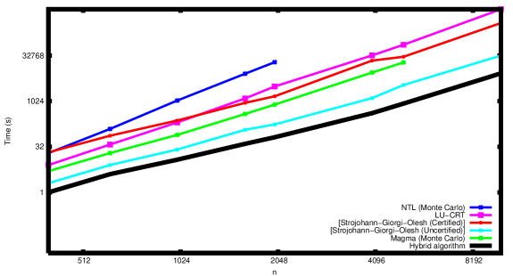
Figure 1: Comparison of our algorithm with other existing implementation. Tested on random dense matrices of the order 400 to 10000, with entries {-8,-7,…,7,8} Using fast modular routines puts our algorithm several times ahead of the others. Scaling is logarithmic.

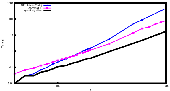
Figure 2: Comparison of our algorithm with early terminated Chinese remaindering algorithm (LU) and the algorithm of Abbott et al. [1] (LIF). Tested on random dense matrices of the order 40 to 1000, with entries {-100,-99,…,99,100}. When matrix size exceeds 80 the adaptive algorithm wins. Scaling is logarithmic.

Thank to the introspective approach our algorithm can detect the cases when the number of invariant factors is small and equal to $k<i_{max}$ . One can therefore argue the complexity of our algorithm is in fact $O\left(n^{3}\left(\log\left(n\right)+\log\left(\|A\|\right)\right)^{2}k\right)$, where $k$ is the number of invariant factors. To test the performance of our algorithm to detect propitious cases we have run it on various sets of structured and engineered matrices. The adaptive approach allowed us to obtain very good timings which motivates us to encourage the use of this algorithms in the situations which go further beyond the dense case.

Figure 3 we present the results of the determinant computation for sparse matrices of N. Trefethen.

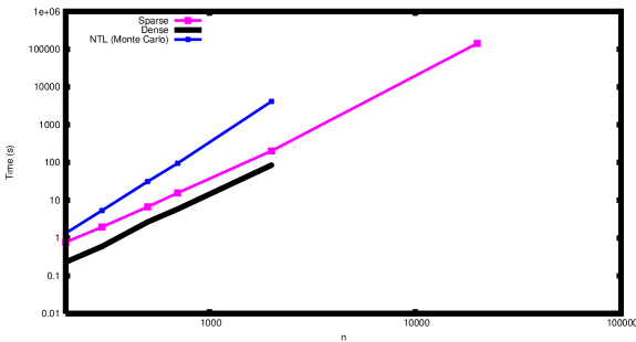
Figure 3: Comparison of sparse and dense variants of our determinant algorithm for Trefethen’s matrices. Scaling is logarithmic.

The results encouraged us to construct a sparse variant of our algorithm, which we shortly describe in Section 5.2. Figure 3 gives a comparison of the performance of sparse and dense variants. We used the sparse solver of [18]. Using the algorithm with the dense solver outperforms using the sparse solver by a factor of $3.3$ to $2.3$, and decreasing with the matrix size $n$. Thanks to the space-efficiency of the sparse algorithm we are able to compute the determinant for $20000\times 20000$ matrix for which the dense solver requires to much memory.

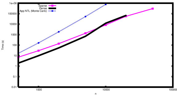
Figure 4: Comparison of sparse and dense variants of our determinant algorithm with the CRA algorithm for random sparse matrices. Scaling is logarithmic. The running time of the CRA algorithm has been approximated based on the timings for one iteration

In figure 4 we compare the performance of dense and sparse variants of the algorithm with the CRA algorithm (sparse variant) for random sparse matrices. The matrices are very sparse (20 non-zero entries per row). To ensure that the determinant is non-zero we put 1 on the diagonal. Both dense and sparse variants of the algorithm have better running times than the CRA, which proves that we can detect propitious cases for sparse matrices. Furthermore, sparse variant is best for bigger matrices and again lets us solve the problem when the dense variant fails due to unsufficient memory.

In Table 1 we give the timings for the algorithm with $i_{max}=1$ and $2$. The algorithms was run on a set of specially engineered matrices which have the same Smith form as $diag\{1,2\dots n\}$ and the number of invariant factors of about $\frac{n}{2}$. We notice that the algorithm with $i_{max}=1$ (which is in fact a slightly modified version of Abbott’s algorithm [1]) runs better for small $n$. This motivated us to develop an even more adaptive approach, which we describe in Section 5.3.

n	$i_{max}=1$	$i_{max}=2$	n	$i_{max}=1$	$i_{max}=2$
100	0.17	0.22	300	5.65	5.53
120	0.29	0.33	350	9.76	9.64
140	0.48	0.55	400	14.99	14.50
160	0.73	0.78	600	57.21	54.96
180	1.07	1.16	800	154.74	147.53
200	1.49	1.51	1000	328.93	309.61
250	2.92	3.00	2000	3711.26	3442.29

Table 1: Comparison of the performance of Algorithm 1 with $i_{\max}$ set to 1 and 2 on engineered matrices.

5.2 Sparse matrix case

When trying to adapt our determinant algorithm to the sparse case, the immediate problem is the bound for the expected number of invariant factors. On can easily notice, that for a matrix with $k$ non-zero entries per row, chosen uniformly and randomly from the set of $S$ contiguous integers, the expected number of invariant factors divisible by $p^{l}$ can be bounded from below by $n\frac{1}{S}\lfloor\frac{S}{p^{l}}\rfloor$ and thus is linear with $n$. Thus, we cannot use the same argument to estimate the expected number of system solvings as in the dense case.

One solution would be to consider the number of ”big” invariant factors, i.e. the number of invariant factors which are bigger than a certain parameter $C$. The parameter has to be chosen in a way, that the product of all smaller factors can be computed by modular CRA loop quicker than another rational solution of a system of equation. We could exploit here the difference in complexity between system solving and one modular routine which is $O^{\sim}\left(n^{3}\right)$ to $O(n^{\omega})$ (or $O(n^{1.5}\Omega)$ to $O(\Omega n)$ in the case of sparse procedures). This could enable us to recover $O\left(n^{3-\omega}\right)$ ($O(n^{0.5})$) bits of the determinant by running modular routines without exceeding the cost of one linear system solving. This adaptive solution is already implemented in the dense version of the algorithm, which motivated us to run it on potentially unsuitable matrices. When comparing the times for the CRA algorithm and our algorithm applied to sparse matrices (however, without exploiting their sparsity) we decided that there is a need for a ”sparse” version of our algorithm, which will take into account the sparse structure of the matrices in the subroutines.

In what follows we will shortly present the sparse counterparts of the subroutines used, give their complexities and discuss some modification of the parameters if needed. We assume that the cost of one matrix-vector product is $\Omega=O\left(n\right)$.

Instead of the dense LU, sparse elimination can be used in practice e.g. for extremely sparse matrices [11]. In general, black box method are preferred. The idea is to precondition the matrix so that its characteristic polynomial equals its minimal polynomial [16, 2]; and then to compute the minimal polynomial via Wiedemann’s algorithm [29]. The complexity of the sparse modular determinant computation is then $O\left(\Omega n\right)$ [11, Table 4]. Adaptive solutions exist [15].

For solving a sparse system of linear equations the solver of [18] can be used. By similar reasoning as in [22], the cost of solving $Ax=b$ for a sparse matrix $A$ is that of $O\left(n^{1.5}\log(n\|A\|)+n^{0.5}\log(\|b\|)\right)$ matrix-vector products and $O\left(n^{2}\log(n\|A\|)\left(n^{0.5}+\log(\|A\|)\right)+n^{2}\log(\|b\|)\log(n\|A\|)+n\log^{2}(\|b\|)\right)$ additional arithmetic operations.

If $\|b\|$ is $O\left(n^{0.5}\right)$ in size and $\Omega=O(n)$, this means that the complexity of computing $s_{n}$ is $O\big{(}n^{2}\log(n\|A\|)(n^{0.5}+\log(\|A\|))\big{)}$ bit operations.

Currently known sparse determinant algorithms that can be used in the worst-case step include the CRA loop (with the complexity $O\left(\Omega n\log(|\det(A)|)\right)$) and the algorithm of [17]. By moving to the sparse solver in [17] we can obtain an algorithm with the worst time complexity of $O\big{(}n^{3}\log^{1.5}(n\|A\|)\log\left(\|A\|\right)\log^{2}\left(n\right)\big{)}$.

All in all, by moving to the sparse procedures, we obtain the algorithm with the complexity $O\left(\min\left(k\left(\Omega n^{1.5}\log(n\|A\|)+n^{2.5}\log(n\|A\|)\log(\|A\|)\right),n^{2}\log(n\|A\|)\Omega\right)\right)$ where $k$ is the number of invariant factors. In the propitious case where $k$ is smaller than $O\left(\sqrt{n}\right)$ we obtain an algorithm with the running time better than the currently known algorithms.

5.3 More adaptivity

We start with a simple remark. For every matrix, with each step, the size of $s_{n-i}$ decreases whilst the cost of its computation increases. In Table 1, this accounts for better performance of Abbott’s algorithm, which computes only $s_{n}$, in the case of small $n$. For bigger $n$ calculating $s_{n-1}$ starts to pay out. The same pattern repeats in further iterations.

The switch between winners in Table 1 can be explained by the fact that, in some situations, obtaining $s_{n-i}$ by $LU$-factorization (which costs $\frac{\log\left(s_{n-i}\right)}{\log\left(l\right)}$ the time of LU) outperforms system solving. Then, this also holds for all consecutive factors and the algorithm based on CRA wins. The condition can be checked a posteriori by approximating the time of LUs needed to compute the actual factor. We can therefore construct a condition that would allow us to turn to the CRA loop in the appropriate moment. This can be done by changing the condition in line 27 ($\tilde{\pi}_{i}=\tilde{\pi}_{i-1}$) to

$$\log\left(\frac{\tilde{\pi}_{i}}{\tilde{\pi}_{i-1}}\right)\leq\frac{time\left(solving\right)}{time\left(LU\right)}\log\left(l\right),$$

if the primes used in the CRA loop are greater than $l$. This would result with a performance close to the best and yet flexible.

If, to some extend, $s_{n-i}$ could be approximated a priori, this condition could be checked before its calculation. This would require a partial factorization of $s_{n-i+1}$ and probability considerations as in section 3.1 and [17].

6 Conclusions

In this paper we have presented an algorithm computing the determinant of an integer matrix. In the dense case we proved that the expected complexity of our algorithm is $O\big{(}n^{3}\log^{2}(n\|A\|)\log^{0.5}\left(n\right)\big{)}$ and depends mainly on the cost of the system solving procedure used and the expected number of invariant factors. Our algorithm uses an introspective approach so that its actual expected complexity is only $O\left(n^{3}\left(\log(n)+\log(\|A\|)\right)^{2}k\right)$ if the number $k$ of invariant factors is smaller than a priori expected but greater than $i_{min}$; The actual running time can be even smaller, assuming that any under-estimation resulting from probabilistically correct procedures can be compensated sooner than expected. Moreover, the adaptive approach allows us to switch to the algorithm with best worst case complexity if it happens that the number of nontrivial invariant factors is unexpectedly large. This adaptivity, together with very fast modular routines, allows us to produce an algorithm, to our knowledge, faster by at least an order of magnitude than other implementations.

Ways to further improve the running time are to reduce the number of iterations in the solvings or to group them in order to get some block iterations as is done e.g. in [3]. A modification to be tested, is to try to reconstruct $s_{n}$ with only some entries of the solution vector $x=\mathbf{n}/d$.

Parallelization can also be considered to further modify the algorithm. Of course, all the LU iterations in one CRA step can be done in parallel. An equivalently efficient way is to perform several $p$-adic liftings in parallel, but with less iterations [8]. There the issue is to perform an optimally distributed early termination.

Appendix A Properties of matrices with almost uniformly distributed entries

In this appendix we present some probabilistic properties of matrices with entries almost uniformly distributed modulo $p^{l}$, $l\in\mathbb{Z}$. We consider the case, when the entries are randomly and uniformly chosen from a set of $S$ contiguous integers $\mathcal{S}=\{a,a+1\dots a+S-1\}$, for any $a$. As the result, the probability that an entry is equal to a given $d$ modulo $p^{l}$ is bounded as follows

$$\frac{1}{S}\lfloor\frac{S}{p^{l}}\rfloor\leq\mathcal{P}(x:x=d\mod p^{l})\leq\frac{1}{S}\lceil\frac{S}{p^{l}}\rceil.$$ (4)

We set

$$\beta=\frac{1}{S}\lceil\frac{S}{p^{l}}\rceil,\quad\alpha=\frac{1}{S}\lfloor\frac{S}{p^{l}}\rfloor.$$ (5)

This special case of non-uniformly distributed random variables was widely considered in the thesis of Z. Wan (see [28]) for $l=1$. In the following we will first consider the rank modulo $p$ of a matrix under certain conditions (lemma A.1). Then we give the analogues of the theorems 5.9-5.15 of [28] in the case $l>1$ (lemmas A.2,A.3, A.4). This allows us to prove Theorem 3.2 on the expected number of invariant factors and Theorem 3.10, which gives the expected size of over-approximation of $\mu_{i}$ in the case of perturbed matrices.

Lemma A.1.

Let $A$ be a $k\times n$, $k\leq n$ integer matrix with entries chosen uniformly and randomly form $\mathcal{S}$. The probability that $\operatorname{rank}_{p}(A)$, the rank modulo $p$ of $A$, is $j$, $0<j\leq k$ is less than or equal to

$$\mathcal{P}\left(\operatorname{rank}_{p}(A)=j\right) \leq\prod_{i=0}^{j-1}(1-\alpha^{(n-i)})\cdot\beta^{(n-j)(k-j)}\cdot\left(\frac{1}{1-\beta}\right)^{\max(k-j-1,0)}(1+\beta\dots\beta^{k-j})$$

$$\leq\beta^{(n-j)(k-j)}\left(\frac{1}{1-\beta}\right)^{k-j},$$ (6)

where $\alpha=\frac{1}{S}\lfloor\frac{S}{p}\rfloor$ and $\beta=\frac{1}{S}\lfloor\frac{S}{p}\rfloor$.

Proof.

The proof is inductive on $k-j$ and $j$. For $j=0$ and $k\ leqn$ the fact that $\operatorname{rank}_{p}(A)=0$ means that all the entries of $A$ are zero modulo $p$, that is

$$\mathcal{P}(\operatorname{rank}_{p}(A)=0)\leq\beta^{nk},$$

the latter being less than $\beta^{nk}\left(\frac{1}{1-\beta}\right)^{k}$.

Now, denote by $A_{i}$ the submatrix of $A$ consisting of $i$ first columns. For $k=j$ we have

$$\mathcal{P}(\operatorname{rank}_{p}(A_{k})=k)=\mathcal{P}(\operatorname{rank}_{p}(A_{k})=k~{}|~{}\operatorname{rank}_{p}(A_{k-1}=k-1))\cdot\mathcal{P}(\operatorname{rank}_{p}(A_{k-1}=k-1)$$

$$=\mathcal{P}(\operatorname{rank}_{p}(A_{1})=1)\prod_{i=2}^{k}\mathcal{P}(\operatorname{rank}_{p}(A_{i})=i~{}|~{}\operatorname{rank}_{p}(A_{i-1}=i-1)).$$

To compute $\mathcal{P}(\operatorname{rank}_{p}(A_{i})=i~{}|~{}\operatorname{rank}_{p}(A_{i-1})=i-1)$ we notice the fact that $\operatorname{rank}_{p}(A_{i-1})=i-1$ means that we can choose an $(i-1)\times(i-1)$ non-zero minor of $A_{i-1}$. This means that we can leave the choice of the corresponding $i-1$ entries of the $i$th column free and only have to ensure that the remaining subvector of size $n-i+1$ is not equal to some given vector. This gives

$$\mathcal{P}(\operatorname{rank}_{p}(A_{i})=i~{}|~{}\operatorname{rank}_{p}(A_{i-1}=i-1)\leq(1-\alpha^{n-i+1})$$

and in consequence

$$\mathcal{P}(\operatorname{rank}_{p}(A_{k})=k)\leq\prod_{i=1}^{k}(1-\alpha^{n-i+1}).$$

Now, assume that for all $(j,k)$ such that $k-j<M$ the bound (A.1) holds. We consider $\mathcal{P}(\operatorname{rank}_{p}(A_{K})=J)$, where $K-J=M>0$. We can rewrite:

$$\mathcal{P}(\operatorname{rank}_{p}(A_{K})=J)=\mathcal{P}(\operatorname{rank}_{p}(A_{K})=J~{}|~{}\operatorname{rank}_{p}(A_{K-1})=J)\cdot\mathcal{P}(\operatorname{rank}_{p}(A_{K-1})=J)$$

$$+\mathcal{P}(\operatorname{rank}_{p}(A_{K})=J~{}|~{}\operatorname{rank}_{p}(A_{K-1})=J-1)\cdot\mathcal{P}(\operatorname{rank}_{p}(A_{K-1})=J-1).$$

To estimate $\mathcal{P}(\operatorname{rank}_{p}(A_{K})=J~{}|~{}\operatorname{rank}_{p}(A_{K-1})=J-1)$, as in previous reasoning, we only have to ensure that $n-J+1$ entries of the last column are not equal to a certain vector. On the contrary, for $\mathcal{P}(\operatorname{rank}_{p}(A_{K})=J~{}|~{}\operatorname{rank}_{p}(A_{K-1})=J)$ we notice that we can leave the choice of $J$ entries corresponding to a non-zero minor free, but the remaining $n-J$ entries have to be determined modulo $p$. By induction, we have

$$\mathcal{P}(\operatorname{rank}_{p}(A_{K})=J)\leq(1-\alpha^{n-J+1})\cdot\prod_{i=0}^{J-2}(1-\alpha^{(n-i)})\cdot\beta^{(n-J+1)(K-J)}\left(\frac{1}{1-\beta}\right)^{K-J-1}$$

$$+\beta^{n-J}\prod_{i=0}^{J-1}(1-\alpha^{(n-i)})\cdot\beta^{(n-J)(K-J-1)}\cdot\left(\frac{1}{1-\beta}\right)^{K-J-1}(1+\beta\dots\beta^{k-j-1})$$

$$=\prod_{i=0}^{J-1}(1-\alpha^{(n-i)})\cdot\beta^{(n-J)(K-J)}\left(\frac{1}{1-\beta}\right)^{K-J-1}(1+\beta\dots\beta^{K-J})$$

which finishes the proof. ∎

Let us consider the example of $n\times 2$ $\{0,1\}$ matrices. We will consider $\alpha=\beta=\frac{1}{2}$. We can construct $2^{2n}$ different matrices, $3\cdot(2^{n}-1)$ of which fulfill the condition that the rank is equal to $1$. The probability of choosing at random a matrix of rank $1$ is thus $\frac{3(2^{n}-1)}{2^{2n}}$. The bound given by Eq. (A.1) is $(1-\left(\frac{1}{2}\right)^{n})\cdot\left(\frac{1}{2}\right)^{n-1}\cdot(1+\frac{1}{2})$ which gives exactly the same value.

The following lemma gives analogues to lemmas 5.10, 5.11 in [28] in the case of the ring $\mathbb{Z}_{p^{l}}$. It proves that the vectors of elements from $\mathcal{S}$ can also be treated as almost-uniformly distributed.

Lemma A.2.

1. Let $t$ be a non-zero mod $p$ vector of size $n$, $d\in\mathbb{Z}_{p^{l}}$. Then the probability that a random vector $x\in\mathcal{S}^{n}$ is chosen such that $t\cdot x=d\mod p^{l}$ is

   $$\mathcal{P}\left(x:t\cdot x=d\mod p^{l}\right)\leq\frac{1}{S}\lceil\frac{S}{p^{l}}\rceil$$

2. Let $A\in\mathbb{Z}^{m\times n}$, a matrix of rank $r$ such that the local Smith form of $A$ at $p$ is trivial, $b\in\mathbb{Z}_{p^{l}}^{m}$ be given. Then the probability that a random vector $x\in\mathcal{S}^{m}$ is chosen such that $Ax=b\mod p^{l}$ is

   $$\mathcal{P}\left(x:Ax=b\mod p^{l}\right)\leq\left(\frac{1}{S}\lceil\frac{S}{p^{l}}\rceil\right)^{r}.$$

Proof.

For (i) the proof of 5.10 from [28] carry on. For (ii) we slightly modify the proof of 5.11 from [28]. Since $A$ has a trival Smith form modulo $p$ there exist two matrices $L,R$, $\det(L),\det(R)\neq 0\mod p$, such that $A=L\left[\begin{array}[]{cc}I_{r}&0\\ 0&0\end{array}\right]\left[\begin{array}[]{c}R^{\prime}\\ R^{\prime\prime}\end{array}\right]$, where $R^{\prime}=[R_{ij}]$ mod $p$ is a $r\times m$ matrix. We may therefore transform

$$\mathcal{P}(x:Ax=b)=\mathcal{P}(x:R^{\prime}x=[L^{-1}b]_{1..r})$$

Since the determinant of $R$ is non-zero modulo $p$ there exist a $r\times r$ minor $R_{1}$ which is non-zero modulo $p$. This means that we can find elements $r_{1i_{1}}\dots r_{1i_{r}}$ of $R_{1}$, where $i_{k}$ are pairwise distinct, such that $r_{ki_{k}}$ are non-zero modulo $p$. Let $d=L^{-1}b$. The probability can be further rewritten:

$$\mathcal{P} (x:R^{\prime}x=[d]_{1..r})=\sum_{j_{1}\in\mathbb{Z}_{p^{l}}}\dots\sum_{j_{r}\in\mathbb{Z}_{p^{l}}}$$

$$\mathcal{P}\left(\begin{array}[]{c}R_{11}x_{1}+\dots+\hat{R_{1i_{1}}x_{i_{1}}}+\dots R_{1n}x_{n}=j_{1}\\ R_{21}x_{1}+\dots+\hat{R_{2i_{2}}x_{i_{2}}}+\dots R_{2n}x_{n}=j_{2}\\ \dots\\ R_{r1}x_{1}+\dots+\hat{R_{ri_{r}}x_{i_{r}}}+\dots R_{rn}x_{n}=j_{r}\end{array}\right)\mathcal{P}\left(\begin{array}[]{c}x_{i_{1}}=(d_{1}-j_{1})R_{1i_{1}}^{-1}\\ x_{i_{2}}=(d_{2}-j_{2})R_{2i_{2}}^{-1}\\ \dots\\ x_{i_{r}}=(d_{r}-j_{r})R_{ri_{r}}^{-1}\end{array}\right)\leq\left(\frac{1}{S}\lceil\frac{S}{p^{l}}\rceil\right)^{r}$$ (15)

We use $\hat{R_{ki_{k}}x_{i_{k}}}$ to denote that the element with index $k$ is omitted in the sum. ∎

The following lemmas show that matrices of elements of $\mathcal{S}$ can be treated as almost uniformly distributed.

Lemma A.3.

Let $L,R\in\mathbb{Z}^{n\times n}$ be matrices such that $|\det\left(L\right)|=|\det\left(R\right)|=1$. Let $\mathcal{I}$, $\mathcal{J}$ be any disjoint subsets of $\{1\dots n\}^{2}$ (sets of index pairs). Let $d_{ij},(i,j)\in\mathcal{I}$ (resp. $D_{st},(s,t)\in\mathcal{J}$) be any values (resp. subsets) from $Z_{p^{l}}$. We consider the probability of choosing a random matrix $X$ such that $\left(LXR\right)_{ij}=d_{ij}$ for $\left(i,j\right)\in\mathcal{I}$ under the condition that $(LXR)_{st}\in D_{st}$ for $\left(s,t\right)\in\mathcal{J}$. We have

$$\mathcal{P}\left(\left(LXR\right)_{ij}=d_{ij}~{}|~{}\left(LXR\right)_{st}\in D_{st}\right)\leq\left(\frac{1}{S}\lceil\frac{S}{p^{l}}\rceil\right)^{|\mathcal{I}|}.$$

Proof.

$$\mathcal{P}\left(\left(LXR\right)_{ij}=d_{ij}~{}|~{}\left(LXR\right)_{st}\in D_{st}\right)=\frac{\mathcal{P}\left(\left(LXR\right)_{ij}=d_{ij}\wedge\left(LXR\right)_{st}\in D_{st}\right)}{\mathcal{P}\left(\left(LXR\right)_{st}\in D_{st}\right)}$$ (16)

Let $\mathcal{D^{\prime}}$ denote a set of all possible matrices $[a_{lk}]$ such that $a_{lk}\in D_{lk}$ if $(l,k)\in\mathcal{J}$ and $a_{lk}\in\mathcal{S}$ otherwise. Let $\mathcal{D}$ denote a set of matrices from $\mathcal{D^{\prime}}$ for which additionally $a_{lk}=d_{lk}$ if $(l,k)\in\mathcal{I}$. Then Eq. (16) can be transformed to

$$\frac{\mathcal{P}\left(X\in L^{-1}\mathcal{D}R^{-1}\right)}{\mathcal{P}\left(X\in L^{-1}\mathcal{D^{\prime}}R^{-1}\right)}$$

Notice, that sets $\mathcal{D}$ and $L^{-1}\mathcal{D}R^{-1}$ (resp. $\mathcal{D^{\prime}}$ and $L^{-1}\mathcal{D^{\prime}}R^{-1}$) have the same number of elements. To compute the probability it suffices to count the number of elements in $\mathcal{D}$ and $\mathcal{D^{\prime}}$. The proportion is determined by the choice of elements from $\mathcal{I}$ and is therefore less than or equal to $\left(\frac{1}{S}\lceil\frac{S}{p^{l}}\rceil\right)^{|\mathcal{I}|}$.

∎

The methods used to prove Lemmas A.2 and A.3 can applied to prove the following lemma.

Lemma A.4.

Let $A\in\mathbb{Z}^{m\times n}$ be a matrix such that the Smith form of $A$ is trivial and $\operatorname{rank}(A)=m\leq n$. Let $\mathcal{I}$, $\mathcal{S}$ be any disjoint subsets of $\{1\dots m\}^{2}$ (sets of index pairs). Let $b_{ij},(i,j)\in\mathcal{I}$ ($B_{st},(s,t)\in\mathcal{S}$) be any values (resp. subsets) from $Z_{p^{l}}$. We consider the probability of choosing a random matrix $X$ such that such that $\left(AX\right)_{ij}=b_{ij}$ for $\left(i,j\right)\in\mathcal{I}$ under the condition that $(LXR)_{st}\in B_{st}$ for $\left(s,t\right)\in\mathcal{S}$. We have

$$\mathcal{P}\left(\left(AX\right)_{ij}=b_{ij}~{}|~{}\left(AX\right)_{st}\in B_{st}\right)\leq\left(\frac{1}{S}\lceil\frac{S}{p^{l}}\rceil\right)^{|\mathcal{I}|}.$$ (17)

Proof.

Let matrices $L,R=R^{\prime}$ be as in the proof of A.2. As in the proof of A.3, we construct the sets of matrices $\mathcal{D}$, $\mathcal{D^{\prime}}$. We have

$$\mathcal{P}\left(\left(AX\right)_{ij}=b_{ij}~{}|~{}\left(AX\right)_{st}\in B_{st}\right)=\frac{\mathcal{P}\left(RX\in L^{-1}\mathcal{D}\right)}{\mathcal{P}\left(RX\in L^{-1}\mathcal{D^{\prime}}\right)}=\frac{\prod_{i=1\dots m}RX_{i}\in L^{-1}\mathcal{D}_{i}}{\prod_{i=1\dots m}RX_{i}\in L^{-1}\mathcal{D^{\prime}}_{i}},$$

where $X_{i}$ denote the $i$th column of $X$ and $\mathcal{D}_{i}(\mathcal{D^{\prime}}_{i})$, the set of all possible $i$th columns for matrices from $\mathcal{D}(\mathcal{D^{\prime}})$. Since (A) holds for every vector $L^{-1}d$ of $L^{-1}\mathcal{D}_{i}(resp.L^{-1}\mathcal{D^{\prime}}_{i})$, again, we can link the the probability to the number of elements in $\mathcal{I}$ and conclude that (17) holds. ∎

We conclude with the following lemma.

Lemma A.5.

Let $V$ be an $k\times n$ matrix, $k\leq n$, such that the Smith form of $V$ is trival and $V$ has a full rank. Let $M$ be an $n\times k$ matrix with entries chosen randomly and uniformly from set $\mathcal{S}$, the probability that $p^{l}<S$ divides the determinant $\det(VM)$ is at most $\frac{3}{p^{l}}$.

Proof.

To check whether $\operatorname{ord}_{p}\left(\det\left(M\right)\right)\geq l$ we will consider a process of diagonalization for $M(0)=VM$ mod $p^{l}$ as described in Algorithm LRE of [7]. It consists of diagonalization and reduction steps. At the $r$-th diagonalization step, if an invertible entry is found, it is placed in the $\left(r,r\right)$ pivot position and the $r$th column is zeroed. If no invertible entry is found, we proceed with a reduction step i.e. we consider the remaining $\left(n-r+1,n-r+1\right)$ submatrix divided by $p$. The problem now reduces to determining whether $\operatorname{ord}_{p}$ of an $\left(n-r+1,n-r+1\right)$ matrix is greater than $l-n+r-1$.

We can consider matrix $M(0)=M_{0}+pM_{1}+p^{2}M_{2}\dots+p^{l}M_{l-1}$, where matrix $M_{k}\in\mathbb{Z}_{p}^{n\times n}$, $k=0\dots l-2$ and $M_{l-1}\in\mathbb{Z}^{n\times n}$. The probability that an entry of $M_{k}$ is equal to a certain $d$ modulo $p$ is less that or equal $\frac{1}{N_{k}}\lceil\frac{N_{k}}{p}\rceil$, where $N_{k}$ is equal to $\lceil\frac{S}{p^{k}}\rceil$ by Lemma A.4.

In the process of diagonalization we can find matrices $L_{0}$, $R_{0}$, $\det\left(L_{0}\right)=\det\left(R_{0}\right)=1$ such that $L_{0}M_{0}R_{0}=\operatorname{diag}\left(\underbrace{1\dots 1}_{r},0\dots 0\right)$ and $L_{0}MR_{0}=\operatorname{diag}\left(\underbrace{1\dots 1}_{r},pL_{0}M_{1}R_{0}+\dots\right)$. Then after the reduction step we set $M_{0}\left(1\right)=[(L_{0}M_{1}R_{0})_{ij}]_{i=r+1\dots n,j=r+1\dots n}$ and $M_{k}\left(1\right)$ equal to $[(L_{0}M_{k+1}R_{0})_{ij}]_{i=r+1\dots n,j=r+1\dots n}$, $M\left(1\right)=M_{0}\left(1\right)+pM_{1}\left(1\right)+\dots$ and we repeat the diagonalization phase. By construction, the choice of $L_{0},\dots L_{k-1},R_{0},\dots R_{k-1}$ means that certain entries of $M$ are fixed and places us in the situation of Lemmas A.3,A.4. Thanks to that we can consider the distribution of entries of $M(k)$ as non-uniform i.e. $\mathcal{P}\left(M(k)_{ij}=d_{ij}\mod p^{\alpha}~{}|~{}L_{0}\dots L_{k-1},R_{0}\dots R_{k-1}\right)\leq\frac{1}{N_{k}}\lceil\frac{N_{k}}{p^{\alpha}}\rceil$.

Another way to see this is to think of the diagonalization as the modification to $a_{22}$ in the form of $a_{22}-\frac{a_{21}}{a_{11}}a_{12}$ with $a_{11}$ and $a_{12}$ fixed by the previous step. Then one has one degree of freedom, say for $a_{21}$ and then $a_{22}$ has to be fixed.

We need only to consider $l-2k$ reductions steps as each reduction is performed on a matrix of order at least 2 and divides the determinant by at least $p^{2}$. Since $k$ is less than $\lceil l/2\rceil-1$ and $l\leq\log_{p}\left(S\right)$, we have $N_{k}\geq\frac{S}{p^{k}}\geq\sqrt{S}$ and since we only consider $p^{\alpha}<N_{k}$ we have

$$\beta_{\alpha}\left(k\right)=\frac{1}{N_{k}}\lceil\frac{N_{k}}{p^{\alpha}}\rceil\leq\frac{N_{k}+p^{\alpha}-1}{p^{\alpha}N_{k}}\leq\frac{2p^{\alpha}}{p^{\alpha}\left(p^{\alpha}+1\right)}=\frac{2}{p^{\alpha}+1}$$

throughout the process. We therefore now set $\beta_{\alpha}=\frac{2}{p^{\alpha}+1}$ and use it as a bound for $\beta_{\alpha}\left(k\right)$, $k=1,2\dots$ in our calculations.

The proof is inductive on $n$, the dimension of the matrix $M\left(k\right)$ and $l$, the current exponent. We fix the diagonalization/reduction matrices $L_{0}\dots L_{k-1},R_{0}\dots L_{k-1}$ and consider the conditional probability $\mathcal{P}^{k-1}=\mathcal{P}\left(\cdot~{}|~{}L_{0}\dots L_{k-1},R_{0}\dots R_{k-1}\right)$.

First, for $l=1$, [28, Thm 5.13] gives

$$\mathcal{P}^{k-1}\left(p\nmid\det\left(M(k)\right)\right)\leq\prod_{i=1}^{n}\left(1-\beta^{i}_{1}\right).$$

This transforms to

$$\mathcal{P}^{k-1}\left(p\mid\det\left(M\left(k\right)\right)\right)\leq\sum_{i=1}^{n}\beta^{i}_{1}\leq\frac{\beta_{1}}{1-\beta_{1}}.$$ (18)

Thus, the probability can be bounded by $\min\left(1,\frac{2}{p-1}\right)$ and therefore by $\frac{3}{p}$.

For $n>1$ we will sum over all possible choices of $L_{k}$ and $R_{k}$. We will divide the sum on the cases when applying $L_{k}$ and $R_{k}$ leads to the diagonalization of at least $r$ entries. We call such an event $E_{r}$.

Then for $n=2,l=2$:

$$\mathcal{P}^{k-1}\left(p^{2}\mid\det\left(M\left(k\right)\right)\right)\leq\sum_{L_{k},R_{k}\in E_{1}}\mathcal{P}^{k-1}\left(p^{2}|\left(L_{k}M\left(k\right)R_{k}\right)_{22}~{}|~{}L_{k},R_{k}\right)\mathcal{P}^{k-1}\left(L_{k},R_{k}\right)$$

$$+\mathcal{P}^{k-1}\left(p|M\left(k\right)_{ij},i,j=1,2\right)\leq\beta_{2}+\beta_{1}^{4}\leq\frac{2}{p^{2}+1}+\left(\frac{2}{p+1}\right)^{4}\leq\frac{3}{p^{2}}$$

Now we suppose inductively that $\mathcal{P}^{k-1}\left(p^{i}\mid\det\left(M\left(k\right)\right)\right)\leq\frac{3}{p^{i}}$ for all $i<l$. Then for $n=2,2<l<n$ the induction gives

$$\mathcal{P}^{k-1}\left(p^{l}\mid\det\left(M\left(k\right)\right)\right)\leq\sum_{L_{k},R_{k}\in E_{1}}\mathcal{P}^{k-1}\left(p^{l}|\left(L_{k}M\left(k\right)R_{k}\right)_{22}~{}|~{}L_{k},R_{k}\right)\mathcal{P}^{k-1}\left(L_{k},R_{k}\right)$$

$$+\mathcal{P}^{k-1}\left(p|M\left(k\right)_{ij},i,j=1,2\right)\mathcal{P}^{k-1}\left(p^{l-2}|\det\left(M\left(k+1\right)\right)\right)\leq\beta_{l}\left(k\right)+\beta_{1}\left(k\right)^{4}\frac{3}{p^{l-2}}.$$

The latter is less than $\frac{3}{p^{l}}$ when

$$\beta_{1}\left(k\right)^{4}3p^{2}\leq 1.$$ (19)

With $\beta_{1}\left(k\right)\leq\frac{2}{p+1}$ this means that $\frac{48}{\left(1+1/p\right)^{2}\left(p+1\right)^{2}}=\frac{48}{\left(p+2+1/p\right)^{2}}\leq 1$ which is fulfilled for $p>3$. For primes $p=2,3$ we have to use a sharper bound for $\beta_{l}\left(k\right)$. Since $p^{l}<N_{k}$ and $l>2$ we have

$$\beta_{1}\left(k\right)\leq\frac{p^{l}+1+p-1}{\left(p^{l}+1\right)p}\leq\frac{p^{l-1}+1}{p^{l}+1}<\frac{p+1}{p^{2}+1}.$$ (20)

This allows us to prove the inequality (19) for $p=3$ since $\left(\frac{2}{5}\right)^{4}27<0.7$. For $p=2$ and $l>3$ also $\left(\frac{9}{17}\right)^{4}12<0.95$ . For the remaining case $p=2$, $l=3$ we can bound $\mathcal{P}^{k-1}\left(p\mid\det\left(M\left(k+1\right)\right)\right)$ by $1$ instead of $\frac{3}{2}$ and then one can prove that $\beta_{3}\left(k\right)+\beta_{1}\left(k\right)^{4}\leq\frac{2}{9}+\left(\frac{5}{9}\right)^{4}<0.32\leq\frac{3}{8}$.

Now we will consider $n>2$. Again we can sum over all possible diagonalization and reduction steps combinations and the resulting bound for the probability is

$$\mathcal{P}^{k-1}\left(p^{l}\mid\det\left(M\left(k\right)\right)\right)\leq\mathcal{P}^{k-1}\left(p|M\left(k\right)_{ij}\forall_{i,j\leq n}\right)$$

$$+\sum_{r=1}^{n-l}\sum_{L_{k},R_{k}\in E_{r}}\mathcal{P}^{k-1}\left(p|\left(L_{k}M\left(k\right)R_{k}\right)_{ij}\forall_{i,j\leq n-r}~{}|~{}L_{k},R_{k}\right)\mathcal{P}^{k-1}\left(L_{k},R_{k}\right)$$

$$+\sum_{r=n-l+1}^{n-2}\sum_{L_{k},R_{k}\in E_{r}}\mathcal{P}^{k-1}\left(p|\left(L_{k}M\left(k\right)R_{k}\right)_{ij}\forall_{i,j\leq n-r}~{}|~{}L_{k},R_{k}\right)\cdot$$

$$\hskip 110.0pt\mathcal{P}^{k-1}\left(L_{k},R_{k}\right)\mathcal{P}^{k}\left(p^{l-n+r}|\det\left(M(k+1)\right)\right)$$

$$+\sum_{L_{k},R_{k}\in E_{n-1}}\mathcal{P}^{k-1}\left(p^{l}|\left(L_{k}M\left(k\right)R_{k}\right)_{nn}~{}|~{}L_{k},R_{k}\right)\mathcal{P}^{k-1}\left(L_{k},R_{k}\right)\leq\sum_{i=l}^{n}\beta_{1}\left(k\right)^{i^{2}}$$

$$+\sum_{r=n-l+1}^{n-2}\sum_{L_{k},R_{k}\in E_{r}}\beta_{1}\left(k\right)^{\left(n-r\right)^{2}}\mathcal{P}^{k-1}\left(L_{k},R_{k}\right)\mathcal{P}^{k}\left(p^{l-n+r}|\det\left(M\left(k+1\right)\right)\right)+\beta_{l}\left(k\right)$$ (21)

for $l\leq n$ and similarly for $l>n$

$$\mathcal{P}^{k-1}\left(p^{l}\mid\det\left(M\left(k\right)\right)\right)\leq\mathcal{P}^{k-1}\left(p|M\left(k\right)_{ij}\forall_{i,j\leq n}\right)\mathcal{P}^{k-1}\left(p^{l-n}|\det\left(M(k+1)\right)\right)$$

$$+\sum_{r=1}^{n-2}\sum_{L_{k},R_{k}\in E_{r}}\mathcal{P}^{k-1}\left(p|\left(L_{k}M\left(k\right)R_{k}\right)_{ij}\forall_{i,j\leq n-r}~{}|~{}L_{k},R_{k}\right)\cdot$$

$$\hskip 95.0pt\mathcal{P}^{k-1}\left(L_{k},R_{k}\right)\mathcal{P}^{k}\left(p^{l-n+r}|\det\left(M(k+1)\right)\right)$$

$$+\sum_{L_{k},R_{k}\in E_{n-1}}\mathcal{P}^{k-1}\left(p^{l}|\left(L_{k}M\left(k\right)R_{k}\right)_{nn}~{}|~{}L_{k},R_{k}\right)\mathcal{P}^{k-1}\left(L_{k},R_{k}\right)$$

$$\leq\beta_{1}\left(k\right)^{n^{2}}\mathcal{P}^{k-1}\left(p^{l-n}|\det\left(M\left(k+1\right)\right)\right)+\beta_{l}\left(k\right)$$

$$+\sum_{r=1}^{n-2}\sum_{L_{k},R_{k}\in E_{r}}\beta_{1}\left(k\right)^{\left(n-r\right)^{2}}\mathcal{P}^{k-1}\left(L_{k},R_{k}\right)\mathcal{P}^{k-1}\left(p^{l-n+r}|\det\left(M\left(k+1\right)\right)~{}|~{}L_{k},R_{k}\right).$$ (22)

Again, we can use the induction to get the bound $\mathcal{P}^{k}\left(p^{l-i}\mid\det\left(M(k+1)\right)\right)\leq\frac{3}{p^{l-i}}$. Then, we can then bound both sums by

$$\mathcal{P}^{k-1}\left(p^{l}\mid\det\left(M\left(k\right)\right)\right)\leq\sum_{i=2}^{\infty}\beta_{1}\left(k\right)^{i^{2}}\frac{3}{p^{l-i}}+\beta_{l}\left(k\right)\leq\frac{3\beta_{1}\left(k\right)^{4}}{p^{l-2}}\frac{1}{\left(1-\beta_{1}\left(k\right)^{5}p\right)}+\beta_{l}\left(k\right).$$ (23)

To prove the inequality $\mathcal{P}^{k-1}\left(p^{l}\mid\det\left(M\left(k\right)\right)\right)\leq\frac{3}{p^{l}}$, we have to consider several cases. For $p>3$ we use the bound $\beta_{1}$ and $\beta_{l}$ for $\beta_{1}\left(k\right)$ and $\beta_{l}\left(k\right)$ respectively. Then we have

$$\frac{3\cdot 2^{4}p^{2}\left(p+1\right)}{p^{l}\left(\left(p+1\right)^{5}-p2^{5}\right)}+\frac{2}{p^{l}+1}<\frac{2}{p^{l}}+\frac{1}{p^{l}}\frac{48p^{2}\left(p+1\right)}{\left(p+1\right)^{5}-\left(p+1\right)2^{4}}<\frac{2}{p^{l}}+\frac{1}{p^{l}}\frac{48p^{2}}{\left(p+1\right)^{4}-2^{4}}$$

$$<\frac{2}{p^{l}}+\frac{1}{p^{l}}\frac{48p^{2}}{25p^{2}+4\cdot 5p^{2}+6\cdot p^{2}+4\cdot 5+1-16}<\frac{2}{p^{l}}+\frac{1}{p^{l}}\frac{48p^{2}}{51p^{2}}<\frac{3}{p^{l}}.$$

For $p=3$ it can be explicitly checked that $\mathcal{P}^{k-1}\left(p^{l}\mid\det\left(M\right)\right)<\frac{3}{p^{l}}$ using the bound $\frac{p+1}{p^{2}+1}$ for $\beta_{1}\left(k\right)$ (notice that $N^{k}>p^{l}$). In this case we get $\frac{1}{3^{l}}\frac{3\left(\frac{2}{5}\right)^{4}3^{2}}{\left(1-\left(3\frac{2}{5}\right)^{5}\right)}+\frac{2}{3^{l}}<\frac{1}{3^{l}}2.75$.

For $p=2$ we have to consider $2^{2},2^{3},2^{4}$ and $2^{l}$ for $l>4$ separately and use the sharper bound from Eq. (20). Let us rewrite (A) and (A) in this cases.

• $l=2$:

  $$\mathcal{P}^{k-1}\left(2^{2}\mid\det\left(M\left(k\right)\right)\right)\leq\sum_{i=2}^{n}\beta_{1}\left(k\right)^{i^{2}}+\beta_{2}\left(k\right)\leq\beta_{1}\left(k\right)^{4}\frac{1}{1-\beta_{1}\left(k\right)^{5}}+\beta_{2}\left(k\right).$$

  As $\beta_{1}\left(k\right)\leq\frac{2+1}{4+1}$ we have $0.65<0.75$.

• $l=3$:

  $$\mathcal{P}^{k-1}\left(2^{3}\mid\det\left(M\left(k\right)\right)\right) \leq\sum_{i=3}^{n}\beta_{1}\left(k\right)^{i^{2}}+\beta_{1}\left(k\right)^{4}\cdot 1+\beta_{3}\left(k\right)$$

  $$\leq\beta_{1}\left(k\right)^{9}\frac{1}{1-\beta_{1}\left(k\right)^{7}}+\beta_{1}(k)^{4}+\beta_{3}(k).$$

  As $\beta_{1}\left(k\right)\leq\frac{4+1}{8+1}$ we have $0.33<0.375$.

• $l=4$:

  $$\mathcal{P}^{k-1}\left(2^{4}\mid\det\left(M(k)\right)\right)\leq\sum_{i=4}^{n}\beta_{1}(k)^{i^{2}}+\beta_{1}(k)^{9}\cdot 1+\beta_{1}(k)^{4}\mathcal{P}^{k}\left(2^{2}\mid\det\left(M(k+1)\right)\right)+\beta_{4}(k)$$

  $$\leq\beta_{1}(k)^{16}\frac{1}{1-\beta_{1}(k)^{9}}+\beta_{1}(k)^{9}+\beta_{1}(k)^{4}\frac{3}{4}+\beta_{4}(k).$$

  As $\beta_{1}\left(k\right)\leq\frac{8+1}{16+1}$ we have $0.18<0.1875$.

• $l>4$:

  We use inequality (23) with $\beta_{1}\left(k\right)$ bounded by $\frac{p^{4}+1}{p^{5}+1}$. We get $\mathcal{P}^{k-1}\left(2^{l}\mid\det\left(M\left(k\right)\right)\right)$ is less than $\frac{1}{2^{l}}\left(\frac{3\left(2^{4}+1\right)^{4}2^{2}}{\left(2^{5}+1\right)^{4}\left(\left(2^{5}+1\right)^{5}\right)-2\left(2^{4}+1\right)}+2\right)<2.92\frac{1}{2^{l}}<\frac{3}{2^{l}}$.

We have thus proven that $\mathcal{P}^{k-1}\left(p^{l}|\det(M(k))\right)\leq\frac{3}{p^{l}}$ for every $l>0$ and every size $n$ of $M(k)$. Thus, $\mathcal{P}(p^{l}|\det(VM))$ is also less than or equal $\frac{3}{p^{l}}$. ∎

References

• [1] J. Abbott, M. Bronstein, T. Mulders. Fast deterministic computation of determinants of dense matrices. In Proc. of ACM International Symposium on Symbolic and Algebraic Computation (ISAAC’1999), 197-204, ACM Press, 1999.
• [2] L. Chen, W. Eberly, E. Kaltofen, B.D. Saunders, W.J. Turner, G. Villard. Efficient matrix preconditioners for black box linear algebra. In Linear Algebra and Applications, pp. 343–344. 2002.
• [3] Z. Chen and A. Storjohann. A BLAS based C library for exact linear algebra on integer matrices. In Proc. of ACM International Symposium on Symbolic and Algebraic Computation (ISAAC’2005), 92–99, ACM Press, 2005.
• [4] D. Coppersmith, S. Winogard. Matrix multiplication via arithmetic progression. In Proc. 19th Annual ACM Symposium of Theory of Computing, 1-6, 1987.
• [5] V.-D. Cung, V. Danjean, J.-G. Dumas, T. Gautier, G. Huard, B. Raffin, C. Rapine, J.-L. Roch, D. Trystram, Adaptive and hybrid algorithms: classification and illustration on triangular system solving, in: Proceedings of Transgressive Computing 2006, Granada, España. 2006.
• [6] J. Dixon. Exact Solution of Linear Equations Using $P$-Adic Expansions. In Numer.Math. 40(1), 137-141, 1982.
• [7] J.G. Dumas, D. Saunders, G. Villard. On Efficient Sparse Integer Matrix Smith Normal Form Computations. In Journal of Symbolic Computations. 32 (1/2), 71-99, 2001.
• [8] J.G. Dumas, W. Turner, Z. Wan. Exact Solution to Large Sparse Integer Linear Systems. ECCAD’2002 : The 9th Annual East Coast Computer Algebra Day, 2002.
• [9] J.G. Dumas, T. Gautier, C. Pernet. FFLAS: Finite field linear algebra subroutines. ISSAC’2002. 2002.
• [10] J.G. Dumas, T. Gautier, M. Giesbrecht, P. Giorgi, B. Hovinen, E. Kaltofen, D. Saunders, W. Turner, G. Villard. LinBox: A Generic Library for Exact Linear Algebra. ICMS’2002 : International Congress of Mathematical Software. 2002.
• [11] J.G. Dumas, G. Villard. Computing the rank of large sparse matrices over finite fields. CASC’2002 Computer Algebra in Scientific Computing. 2002.
• [12] J.G. Dumas, P. Giorgi, C. Pernet. FFPACK: finite field linear algebra package. ISSAC’2004. 2004.
• [13] J.G. Dumas, C. Pernet, Zhendong Wan. Efficient Computation of the Characteristic Polynomial. ISSAC’2005, p 181-188. 2005.
• [14] J.G. Dumas, A. Urbańska. An introspective algorithm for the integer determinant. In: Proceedings of Transgressive Computing 2006, Granada, España. 2006.
• [15] A. Duran, D. Saunders, Z.Wan. Hybrid Algorithms for Rank of Sparse Matrices. In: Proceedings of the SIAM International Conference on Applied Linear Algebra. 2003.
• [16] W. Eberly, E. Kaltofen. On randomized Lanczos algorithms. ISSAC’1997. 1997
• [17] W. Eberly, M. Giesbrecht, G. Villard. On computing the determinant and smith form of an integer matrix. In Proc. 41st FOCS, 675-687, 2000.
• [18] W. Eberly, M.Giesbrecht, P. Giorgi, A. Storjohann, G. Villard. Solving Sparse Integer Linear Systems. ISSAC’2006. 2006.
• [19] O.H. Ibarra, S. Moran, R.Hui. A generalization of the fast LUP matrix decomposition algorithm and applications. Journal of Algorithms, 3(1):452̆01356, Mar.1982.
• [20] E. Kaltofen, G. Villard. Computing the sign or the value of the determinant of an integer matrix, a complexity survey. In Journal of Computational and Applied Mathematics 164(2004), 133-146 2004.
• [21] E. Kaltofen, G. Villard. On the complexity of computing determinants. Computational Complexity, 31(3-4), pp 91–130, 2005.
• [22] T. Mulders, A. Storjohann. Diophantine Linear System Solving. ISAAC’1999, 181-188. 1999.
• [23] D. Musser. Introspective Sorting and Selection Algorithms. Software—Practice and Experience, 8(27), pp 983–993, 1997.
• [24] V. Pan. Computing the determinant and the characteristic polynomial of a matrix via solving linear systems of equations. Inform. Process. Lett. 28(1988) 71-75. 1988.
• [25] D. Saunders, Z. Wan. Smith Normal Form of Dense Integer Matrices, Fast Algorithms into Practice. ISSAC 2004 2004.
• [26] A.Storjohann. The shifted number system for fast linear algebra on integer matrices. Journal of Complexity, 21(4), pp 609–650, 2005.
• [27] A. Storjohann, P. Giorgi, Z. Olesh. Implementation of a Las Vegas integer Matrix Determinant Algorithm. ECCAD’05: East Coast Computer Algebra Day, 2005.
• [28] Z. Wan. Computing the Smith Forms of Integer Matrices and Solving Related Problems. Ph.D. Thesis, U. of Delaware, USA, 2005.
• [29] D. Wiedemann. Solving sparse linear equations over Finite Fields. In IEEE Trans. Inf. Theory, pp. 54-62. 1986.