On-line regression competitive with reproducing kernel Hilbert spaces

Abstract

We consider the problem of on-line prediction of real-valued labels, assumed bounded in absolute value by a known constant, of new objects from known labeled objects. The prediction algorithm’s performance is measured by the squared deviation of the predictions from the actual labels. No stochastic assumptions are made about the way the labels and objects are generated. Instead, we are given a benchmark class of prediction rules some of which are hoped to produce good predictions. We show that for a wide range of infinite-dimensional benchmark classes one can construct a prediction algorithm whose cumulative loss over the first $N$ examples does not exceed the cumulative loss of any prediction rule in the class plus $O(\surd{N})$; the main differences from the known results are that we do not impose any upper bound on the norm of the considered prediction rules and that we achieve an optimal leading term in the excess loss of our algorithm. If the benchmark class is “universal” (dense in the class of continuous functions on each compact set), this provides an on-line non-stochastic analogue of universally consistent prediction in non-parametric statistics. We use two proof techniques: one is based on the Aggregating Algorithm and the other on the recently developed method of defensive forecasting.

• The main difference of the current (second) version of this technical report from the previous version is a fuller discussion of the related literature. The latter is, however, massive, and it is likely that even in this version some important related results are missing.

1 Introduction

The traditional, and still dominant, approach to the problem of regression is statistical: the objects and their real-valued labels are assumed to be generated independently from the same probability distribution, and a typical goal is to find a prediction rule with a small expected loss. A newer approach is “competitive on-line regression”, in which the goal is to perform almost as well as the best rules in a given benchmark class of prediction rules. (See, e.g., [36], §1, or [54], §4, for reviews of some relevant literature.) Unlike the statistical theory of regression, no stochastic assumptions are made about the data.

A great impetus for the development of the statistical theories of regression and pattern recognition (see, e.g., [28] and, especially, [18], Preface and Chapter 1) has been Stone’s 1977 result [49] that there exists a “universally consistent” prediction algorithm: an algorithm that asymptotically achieves, with probability one (or high probability), the best possible expected loss. The property of universal consistency is very attractive, but it is asymptotic and does not tell us anything about finite data sequences. Stone’s result provided a direction in which more practicable results have been sought.

Surprisingly, it appears that universal consistency has not been even defined in competitive on-line learning theory. We propose such a definition in §2; in §5 we will see how close papers such as [15, 6] came to constructing universally consistent algorithms. However, our Corollary 1 in §2 appears to be the first explicit statement about the existence of the latter.

As in the case of statistical regression, universal consistency is only a minimal requirement; one also wants good rates of convergence, ideally not involving unknown constants, for universal benchmark classes. The notion of universality is discussed, formally and informally, at the end of §2 and in §4; we will argue that universality for benchmark classes is a matter of degree. Our main results, Theorems 1–3, are stated in §2 and proved in §§6–8. They describe properties of universality of our prediction algorithms, some of which are described explicitly in the last section, §10. In §3, Theorem 1 is applied to the case where the objects and their labels are drawn independently from the same distribution. In §4 we consider some interesting benchmark classes of prediction rules, and in §5 we compare our results to some related ones in the literature.

In this paper we use two very different proof techniques: the old one introduced in [53, 54] and the one developed in [55]; we are especially interested in the latter since it appears much more versatile, and competitive on-line regression is a good testing ground to develop it. This technique has its origin in Foster and Vohra’s paper [25], which demonstrated the existence of a randomized forecasting strategy that produces asymptotically well-calibrated forecasts with probability one. Foster and Vohra’s result was translated into the game-theoretic foundations of probability (see, e.g., [45]) in [58]. In June 2004 Akimichi Takemura further developed the method of [58] showing that for any continuous game-theoretic law of probability there exists a forecasting strategy that perfectly satisfies this law of probability; such a strategy was called a “defensive forecasting strategy” in [59]. An important special case of defensive forecasting is where the law of probability asserts good calibration and resolution of the forecasts; it was explored in [56], where, in particular, a non-asymptotic version of Foster and Vohra’s result was proved. In [55] it was shown that the corresponding forecasting strategies lead to a small cumulative loss in a fairly wide class of decision protocols. That paper only dealt with the case of binary classification, and in this paper similar results are proved for on-line regression. As the loss function we use square-loss, which leads to significant simplifications as compared with [55]. (Despite [25] being the source of our approach, our proof technique appears to have lost all connections with that paper and papers, such as [37, 42, 43, 32], further developing it.)

Our results are closely related to those of Cesa-Bianchi et al. [15] and Auer et al. [6], but we postpone a detailed discussion to §5.

2 Main results

The simple perfect-information protocol of this section is:

FOR $n=1,2,\dots$:
Reality announces $x_{n}\in\mathbf{X}$.
Predictor announces $\mu_{n}\in\mathbb{R}$.
Reality announces $y_{n}\in[-Y,Y]$.
END FOR.

At the beginning of each round $n$ Predictor is shown an object $x_{n}$ whose label $y_{n}$ is to be predicted. The set of a priori possible objects is called the object space and denoted $\mathbf{X}$; of course, we always assume $\mathbf{X}\neq\emptyset$. After Predictor announces his prediction $\mu_{n}$ for the object’s label he is shown the actual label $y_{n}\in\mathbb{R}$. We assume known an a priori upper bound $Y\in(0,\infty)$ on the absolute values of the labels $y_{n}$. We will sometimes refer to pairs $(x_{n},y_{n})$ as examples. By an on-line prediction algorithm we mean a strategy for Predictor in this protocol; in this paper, however, we are not concerned with computational complexity of our prediction algorithms.

Predictor’s loss on round $n$ is measured by $(y_{n}-\mu_{n})^{2}$, and so his cumulative loss after $N$ rounds of the game is $\sum_{n=1}^{N}(y_{n}-\mu_{n})^{2}$. His goal is “universal prediction”, in the following, rather vague, sense. If $D:\mathbf{X}\to\mathbb{R}$ is a “prediction rule” (i.e., the function $D$ is interpreted as a rule for choosing the prediction based on the current object), he would like to have

$$\sum_{n=1}^{N}(y_{n}-\mu_{n})^{2}\lessapprox\sum_{n=1}^{N}(y_{n}-D(x_{n}))^{2}$$ (1)

($\lessapprox$ meaning “not much greater than”) provided $D$ is not “too complex”. Technically, we will be interested in the case where the prediction rule $D$ is assumed to belong to a large reproducing kernel Hilbert space (to be defined shortly) and the complexity of $D$ is measured by its norm.

As already mentioned, the results of this section are closely related to several results in [15] and [6]; see §5.

Reproducing kernel Hilbert spaces

A reproducing kernel Hilbert space (RKHS) on a set $Z$ (such as $Z=\mathbf{X}$) is a Hilbert space $\mathcal{F}$ of real-valued functions on $Z$ such that the evaluation functional $f\in\mathcal{F}\mapsto f(z)$ is continuous for each $z\in Z$. We will use the notation $\mathbf{c}_{\mathcal{F}}(z)$ for the norm of this functional:

$$\mathbf{c}_{\mathcal{F}}(z):=\sup_{f:\left\|f\right\|_{\mathcal{F}}\leq 1}\left|f(z)\right|.$$

Let

$$\mathbf{c}_{\mathcal{F}}:=\sup_{z\in Z}\mathbf{c}_{\mathcal{F}}(z);$$ (2)

we will be interested in the case $\mathbf{c}_{\mathcal{F}}<\infty$.

Examples of RKHS will be given in §4.

Main theorems

Suppose Predictor’s goal is to compete with prediction rules $D$ from an RKHS $\mathcal{F}$ on $\mathbf{X}$. The three theorems that we state in this subsection bound the difference between the left-hand and right-hand sides of (1); this bound will be called the regret term. The simplest regret term, given in the first theorem, is in terms of $\mathbf{c}_{\mathcal{F}}$, $\left\|D\right\|_{\mathcal{F}}$, and $N$.

Theorem 1

Let $\mathcal{F}$ be an RKHS on $\mathbf{X}$. There exists an on-line prediction algorithm producing $\mu_{n}\in[-Y,Y]$ that are guaranteed to satisfy

$$\sum_{n=1}^{N}(y_{n}-\mu_{n})^{2}\leq\sum_{n=1}^{N}(y_{n}-D(x_{n}))^{2}+2Y\sqrt{\mathbf{c}_{\mathcal{F}}^{2}+1}\left(\left\|D\right\|_{\mathcal{F}}+Y\right)\sqrt{N}$$ (3)

for all $N=1,2,\ldots$ and all $D\in\mathcal{F}$.

The regret term in the second theorem is in terms of $\mathbf{c}_{\mathcal{F}}$, $\left\|D\right\|_{\mathcal{F}}$, and the cumulative loss of $D$ (which can be significantly less than $N$).

Theorem 2

Let $\mathcal{F}$ be an RKHS on $\mathbf{X}$. There exists an on-line prediction algorithm producing $\mu_{n}\in[-Y,Y]$ that are guaranteed to satisfy

$$\sum_{n=1}^{N}(y_{n}-\mu_{n})^{2}\leq\sum_{n=1}^{N}(y_{n}-D(x_{n}))^{2}\\ +2\sqrt{\mathbf{c}_{\mathcal{F}}^{2}+1}\left(\left\|D\right\|_{\mathcal{F}}+Y\right)\sqrt{\sum_{n=1}^{N}(y_{n}-D(x_{n}))^{2}+\left(\mathbf{c}_{\mathcal{F}}^{2}+1\right)\left(\left\|D\right\|_{\mathcal{F}}+Y\right)^{2}}\\ +2\left(\mathbf{c}_{\mathcal{F}}^{2}+1\right)\left(\left\|D\right\|_{\mathcal{F}}+Y\right)^{2}$$ (4)

for all $N$ and all $D\in\mathcal{F}$.

The regret term of Theorem 2 is close to being stronger than that of Theorem 1: the former is at most twice as large as the latter plus an additive constant, if we restrict our attention to the prediction rules $D$ such that $\left\|D\right\|_{\mathcal{F}}$ is bounded by a constant and $\left|D(x)\right|\leq Y$, $\forall x\in\mathbf{X}$.

On-line prediction algorithms achieving (3) and (4) will be stated explicitly in §10. They are based on the idea of defensive forecasting. However, the regression problem considered in this paper is very well studied, and one can hardly hope to beat the known techniques. The next theorem gives an upper bound of the regret term achievable by using the procedure (“Aggregating Algorithm”, or AA) described in [53] and applied to the problem of regression in [54] and [26]. A popular alternative technique based on the gradient descent method could also be used, but it tends to lead to worse leading constants: see §5 for details.

Theorem 3

Let $\mathcal{F}$ be a separable RKHS on $\mathbf{X}$. There exists an on-line prediction algorithm producing $\mu_{n}\in[-Y,Y]$ that are guaranteed to satisfy

$$\sum_{n=1}^{N}(y_{n}-\mu_{n})^{2}\leq\sum_{n=1}^{N}(y_{n}-D(x_{n}))^{2}\\ -2Y^{2}\ln\left(\Gamma\left(\frac{N}{2}+1\right)U\left(\frac{N}{2}+1,0,\frac{\mathbf{c}_{\mathcal{F}}^{2}\left\|D\right\|_{\mathcal{F}}^{2}}{2Y^{2}}\right)\right)\\ \leq\sum_{n=1}^{N}(y_{n}-D(x_{n}))^{2}+2Y\max\left(\mathbf{c}_{\mathcal{F}}\left\|D\right\|_{\mathcal{F}},Y\delta N^{-1/2+\delta}\right)\sqrt{N+2}\\ +\frac{3}{2}Y^{2}\ln N+\frac{\mathbf{c}_{\mathcal{F}}^{2}\left\|D\right\|_{\mathcal{F}}^{2}}{4}+O(Y^{2})$$ (5)

for all $N=1,2,\ldots$ and all $D\in\mathcal{F}$, where $\delta>0$ is an arbitrarily small constant, $\Gamma$ is the gamma function ([1], Chapter 6), and $U$ is Kummer’s $U$ function ([1], Chapter 13). The constant implicit in $O(Y^{2})$ depends only on $\delta$.

The bound of Theorem 3 is even closer to being stronger than that of Theorem 1 as $N\to\infty$: the leading constant is the same, $2Y\mathbf{c}_{\mathcal{F}}\left\|D\right\|_{\mathcal{F}}$ (assuming $\left\|D\right\|_{\mathcal{F}}\gg Y$ and $\mathbf{c}_{\mathcal{F}}\gg 1$), but the other terms are considerably better. The main disadvantage of the bound (5) is the asymptotic character of (namely, the presence of the $O$ term in) its more explicit version. The version involving the gamma and Kummer’s $U$ functions is not intuitive, but it can be evaluated using standard libraries; the function

$$f(N,d):=-\ln\left(\Gamma\left(\frac{N}{2}+1\right)U\left(\frac{N}{2}+1,0,\frac{d^{2}}{2}\right)\right)$$

is plotted in Figure 1.

The condition of separability in Theorem 3 does not appear restrictive; in particular, it is satisfied for all examples considered in §4.

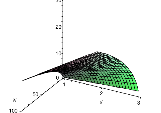
Figure 1: The graph of the function $f(N,d)$ for $N=1,\ldots,100$ and $d\in[1,3]$. The two final values at the corners are $f(100,1)\approx 12.37$ and $f(100,3)\approx 30.15$.

Finally, we give a lower bound (a version of Theorem VII.2 in [15]) showing that the leading constant $2Y\mathbf{c}_{\mathcal{F}}\left\|D\right\|_{\mathcal{F}}$ is optimal.

Theorem 4

Suppose the object space is $\mathbf{X}=\mathbb{R}$. For any positive constant $c$ there exists an RKHS $\mathcal{F}$ on $\mathbf{X}$ with $\mathbf{c}_{\mathcal{F}}=c$ and a strategy for Reality satisfying the following property. For any $N=1,2,\ldots$, any positive constant $d\leq(Y/\mathbf{c}_{\mathcal{F}})\surd N$, and any on-line prediction algorithm, there exists a prediction rule $D\in\mathcal{F}$ such that $\left\|D\right\|_{\mathcal{F}}=d$ and

$$\sum_{n=1}^{N}(y_{n}-\mu_{n})^{2}\geq\sum_{n=1}^{N}(y_{n}-D(x_{n}))^{2}+2Y\mathbf{c}_{\mathcal{F}}\left\|D\right\|_{\mathcal{F}}\sqrt{N}-\mathbf{c}_{\mathcal{F}}^{2}\left\|D\right\|_{\mathcal{F}}^{2},$$ (6)

where, as usual, $\mu_{n}$ are the predictions produced by the on-line prediction algorithm and $(x_{n},y_{n})$ are Reality’s moves.

Theorems 3 and 4 are proved in §8 and §9, respectively. From the proof of Theorem 4 it will be clear that similar lower bounds also hold when $\mathbf{X}=\mathbb{R}$ is replaced by any regular (e.g., open) subset of a Euclidean space.

• If $\mathbf{c}_{\mathcal{F}}=\infty$ but it is known in advance that all objects $x_{n}$, $n=1,2,\ldots$, will be chosen from a set $A\subseteq\mathbf{X}$ satisfying $X:=\sup_{x\in A}\mathbf{c}_{\mathcal{F}}(x)<\infty$, Theorem 1–4 will continue to hold when $\mathbf{c}_{\mathcal{F}}$ is replaced by $X$.

Universal consistency

We say that an RKHS $\mathcal{F}$ on $Z$ is universal if $Z$ is a topological space and for every compact subset $A$ of $Z$ every continuous function on $A$ can be arbitrarily well approximated in the metric $C(A)$ by functions in $\mathcal{F}$; in the case of compact $Z$ this coincides with the definition given in [48] (Definition 4). All examples of RKHS given in §4 are universal.

Suppose the object space $\mathbf{X}$ is a topological space; as in the rest of the paper, we are assuming that $\lvert y_{n}\rvert$ are bounded by a known constant $Y$. Let us say that an on-line prediction algorithm is universally consistent if its predictions $\mu_{n}$ always satisfy

$$\left(x_{n}\in A,\forall n\in\{1,2,\ldots\}\right)\\ \Longrightarrow\limsup_{N\to\infty}\left(\frac{1}{N}\sum_{n=1}^{N}(y_{n}-\mu_{n})^{2}-\frac{1}{N}\sum_{n=1}^{N}(y_{n}-D(x_{n}))^{2}\right)\leq 0$$ (7)

for any compact subset $A$ of $\mathbf{X}$ and any continuous decision rule $D$ (cf. (1)). By the Tietze–Uryson theorem ([19], Theorem 2.6.4 on p. 65), if $\mathbf{X}$ is a normal topological space, we will obtain an equivalent definition allowing $D$ to be any continuous function from $A$ to $\mathbb{R}$.

The definitions of this subsection are most intuitive in the case of compact $\mathbf{X}$, and in our informal discussion we will be making this assumption. The main remaining difference of our definition of universal consistency from the statistical one [49] is that we require $D$ to be continuous. If $D$ is allowed to be discontinuous, (7) is impossible to achieve: no matter how Predictor chooses his predictions $\mu_{n}$, Reality can choose

$$x_{n}:=\sum_{i=1}^{n-1}\frac{\mathop{\rm sign}\nolimits(\mu_{i})}{3^{i}},\quad y_{n}:=\begin{cases}1&\text{if $\mu_{n}<0$}\\ -1&\text{otherwise}\end{cases}$$

(assuming $\mathbf{X}\supseteq[-1,1]$ and $Y\geq 1$), foiling (7) for the prediction rule

$$D(x):=\begin{cases}-1&\text{if $x<\sum_{i=1}^{\infty}\mathop{\rm sign}\nolimits(\mu_{i})/3^{i}$}\\ 1&\text{otherwise}.\end{cases}$$

A positive argument in favor of the requirement of continuity of $D$ is that it is natural for Predictor to compete only with computable prediction strategy, and continuity is often regarded as a necessary condition for computability (Brouwer’s “continuity principle”).

The existence of universal RKHS on Euclidean spaces $\mathbb{R}^{m}$ (see §4) implies the following proposition.

Corollary 1

If $\mathbf{X}\subseteq\mathbb{R}^{m}$ for some $m=1,2,\ldots$, there exists a universally consistent on-line prediction algorithm.

• Any on-line prediction algorithm satisfying (3) of Theorem 1 for a universal RKHS $\mathcal{F}$ on $\mathbb{R}^{m}$ will be universal. Indeed, let $A\subseteq\mathbf{X}$ be compact, $f$ be a continuous function on $\mathbf{X}$, and $\epsilon>0$. Suppose $x_{n}\in A$, $n=1,2,\ldots$ . Our goal is to prove that

  $$\frac{1}{N}\sum_{n=1}^{N}(y_{n}-\mu_{n})^{2}\leq\frac{1}{N}\sum_{n=1}^{N}(y_{n}-f(x_{n}))^{2}+\epsilon$$

  from some $N$ on. It suffices to choose $D\in\mathcal{F}$ at a distance at most $\epsilon/(8Y)$ from $f$ in the metric $C(A)$, apply (3) to $D$, and notice that

  $$\left|\frac{1}{N}\sum_{n=1}^{N}(y_{n}-D(x_{n}))^{2}-\frac{1}{N}\sum_{n=1}^{N}(y_{n}-f(x_{n}))^{2}\right|\leq 4Y\frac{\epsilon}{8Y}=\frac{\epsilon}{2}$$

  (this calculation assumes that $f$ and $D$ take values in $[-Y,Y]$; we can always achieve this by truncating $f$ and $D$: truncation does not lead outside the universal RKHS described in §4).      

• It is easy to extend Corollary 1 to the case where $\mathbf{X}$ is a separable metric space or a compact metric space: indeed, by Theorem 4.2.10 in [20] the Hilbert cube is a universal space for all separable metric spaces and for all compact metric spaces, and every continuous function on the Hilbert cube (we are interested in continuous extensions of continuous functions on compact subsets), being uniformly continuous (see, e.g., [19], Corollary 2.4.6 on p. 52), can be arbitrarily well approximated by functions that only depend on the first $m$ coordinates of their argument; it remains to notice that the on-line prediction algorithms satisfying the condition of Theorem 1 for universal RKHS on $[0,1]^{m}$ can be merged into one on-line prediction algorithm using, e.g., the Aggregating Algorithm.

So far in this subsection we have only discussed the asymptotic notion of universal consistency, although it is clear that one needs universality in a stronger sense. In practical problems, it is not enough for the benchmark class $\mathcal{F}$ to be universal; we also want as many prediction rules $D$ as possible to belong to $\mathcal{F}$, or at least to be well approximated by the elements of $\mathcal{F}$; we also want $\left\|D\right\|_{\mathcal{F}}$ to be as small as possible. The Sobolev spaces on $[0,1]^{m}$ discussed in §4 are not only universal RKHS but also include all functions that are smooth in a fairly weak sense. However, the Hilbert-space methods have their limitations: it is not clear, e.g., how to apply them to functions that are as “smooth” as typical trajectories of the Brownian motion. These larger benchmark classes seem to require Banach-space methods: see [57].

3 Implications for the statistical theory of regression

So far we have not made any stochastic assumptions about the way the examples are produced. In this section we derive simple implications from Theorem 1 for the statistical learning framework, assuming that the examples $(x_{n},y_{n})$ are drawn independently from some probability distribution on $\mathbf{X}\times[-Y,Y]$. Similar implications can be derived from the results of [15], [6], and some other papers (see the next section); the corollary stated in this section, however, has somewhat better constants.

Generalization bounds

The risk of a prediction rule $D:\mathbf{X}\to\mathbb{R}$ with respect to a probability distribution $P$ on $\mathbf{X}\times[-Y,Y]$ is defined as

$$\mathop{\mathrm{risk}}\nolimits_{P}(D):=\int_{\mathbf{X}\times[-Y,Y]}(y-D(x))^{2}P(\mathrm{d}x,\mathrm{d}y).$$

Our goal in this section is to construct, from a given sample, a prediction rule whose risk is competitive with the risk of small-norm prediction rules in a given RKHS. As shown in [13] (with similar results obtained earlier in [11] and before that in [38]), this can be easily done once we have a competitive on-line algorithm (such as those in Theorems 1–3).

Fix an on-line prediction algorithm and a sequence of examples

$$(x_{1},y_{1}),(x_{2},y_{2}),\ldots\,.$$

For each $n=1,2,\ldots$, let $H_{n}:\mathbf{X}\to\mathbb{R}$ be the function that maps each $x\in\mathbf{X}$ to the prediction $\mu_{n}\in\mathbb{R}$ output by the algorithm when fed with $(x_{1},y_{1}),\ldots,(x_{n-1},y_{n-1}),x$. We will say that the prediction rule

$$\overline{H}_{N}(x):=\frac{1}{N}\sum_{n=1}^{N}H_{n}(x)$$

is obtained by averaging from the on-line prediction algorithm.

Corollary 2

Let $\mathcal{F}$ be an RKHS on $\mathbf{X}$, let $D\in\mathcal{F}$ be such that $D(x)\in[-Y,Y]$ for all $x\in\mathbf{X}$, and let $\overline{H}_{N}$, $N=1,2,\ldots$, be the prediction rules obtained by averaging from some on-line prediction algorithm guaranteeing (3). For any probability distribution $P$ on $\mathbf{X}\times[-Y,Y]$, any $N=1,2,\ldots$, and any $\delta>0$,

$$\mathop{\mathrm{risk}}\nolimits_{P}(\overline{H}_{N})\leq\mathop{\mathrm{risk}}\nolimits_{P}(D)+\frac{2Y}{\sqrt{N}}\left(\sqrt{\mathbf{c}_{\mathcal{F}}^{2}+1}\left(\left\|D\right\|_{\mathcal{F}}+Y\right)+2Y\sqrt{2\ln\frac{2}{\delta}}\right)$$ (8)

with probability at least $1-\delta$.

• For a suitable choice of $\epsilon>0$, we will have

  $$\mathop{\mathrm{risk}}\nolimits_{P}(\overline{H}_{N}) \leq\frac{1}{N}\sum_{n=1}^{N}\mathop{\mathrm{risk}}\nolimits_{P}(H_{n})$$ (9)

  $$\leq\frac{1}{N}\sum_{n=1}^{N}(y_{n}-H_{n}(x_{n}))^{2}+\epsilon$$ (10)

  $$\leq\frac{1}{N}\sum_{n=1}^{N}(y_{n}-D(x_{n}))^{2}+\frac{2Y}{\sqrt{N}}\sqrt{\mathbf{c}_{\mathcal{F}}^{2}+1}\left(\left\|D\right\|_{\mathcal{F}}+Y\right)+\epsilon$$ (11)

  $$\leq\frac{1}{N}\sum_{n=1}^{N}\mathop{\mathrm{risk}}\nolimits_{P}(D)+\frac{2Y}{\sqrt{N}}\sqrt{\mathbf{c}_{\mathcal{F}}^{2}+1}\left(\left\|D\right\|_{\mathcal{F}}+Y\right)+2\epsilon$$ (12)

  $$=\mathop{\mathrm{risk}}\nolimits_{P}(D)+\frac{2Y}{\sqrt{N}}\sqrt{\mathbf{c}_{\mathcal{F}}^{2}+1}\left(\left\|D\right\|_{\mathcal{F}}+Y\right)+2\epsilon$$

  with probability at least $1-\delta$. The inequalities (9) and (11) always hold: the first follows from the convexity of the function $t\mapsto t^{2}$, and the second from Theorem 1. By Hoeffding’s martingale inequality ([31], Theorem 1 and the remark at the end of §2; see also [18], Theorem 9.1 on p. 135), (10) and (12) will hold with probability at least $1-e^{-\epsilon^{2}N/(8Y^{4})}$; to make the probability of their conjunction at least $1-\delta$, it suffices to find $\epsilon$ from the equation $e^{-\epsilon^{2}N/(8Y^{4})}=\delta/2$, which gives

  $$\epsilon=\frac{2Y^{2}}{\sqrt{N}}\sqrt{2\ln\frac{2}{\delta}}.$$  

In Corollary 2 we only consider prediction rules taking values in $[-Y,Y]$; this is not a real restriction if the RKHS $\mathcal{F}$ satisfies $D\in\mathcal{F}\Longrightarrow\left|D\right|\in\mathcal{F}$, as the examples of RKHS considered in §4 do.

Universally consistent procedures

Suppose the object space $\mathbf{X}$ is the Euclidean space $\mathbb{R}^{m}$ for some $m$. It is easy to see that Corollary 2 implies the existence of universally consistent procedures in the sense of Stone [49] for a known upper bound $Y$ on $\lvert y_{n}\rvert$. Indeed, by Luzin’s theorem ([19], Theorem 7.5.2 on p. 244; see also Theorem 7.1.3 on p. 225) for any Borel measurable prediction rule $f:\mathbf{X}\to[-Y,Y]$ and any $\epsilon>0$ there exist a closed set $F\subseteq\mathbf{X}$ of probability at least $1-\epsilon$ such that the restriction of $f$ to $A$ is continuous; it is obvious that we can also assume that $F$ is compact. Let $D$ be a function in a universal RKHS on $\mathbf{X}$ (the existence of the latter is shown in §4) taking values in $[-Y,Y]$ and close to $f$ in the metric $C(F)$. It remains to apply Corollary 2.

Intuitively, the statistical assumption that the examples are produced independently from the same distribution is strong enough for the requirement of continuity to be superfluous: as Cover mentioned in his discussion of Stone’s paper, it holds automatically with high probability.

4 Examples of RKHS and reproducing kernels

The usefulness of the results stated in the previous two sections depends on the availability of suitable RKHS. In this section I will only give simplest examples; for numerous other examples see, e.g., [52], [44], and [46].

The Sobolev spaces

The Sobolev norm $\left\|f\right\|_{H^{1}}$ of an absolutely continuous function $f:[0,1]\to\mathbb{R}$ is defined by

$$\left\|f\right\|_{H^{1}}^{2}:=\int_{0}^{1}\left(f(t)\right)^{2}\,\mathrm{d}t+\int_{0}^{1}\left(f^{\prime}(t)\right)^{2}\,\mathrm{d}t.$$ (13)

The Sobolev space $H^{1}([0,1])$ on $[0,1]$ is the set of absolutely continuous $f:[0,1]\to\mathbb{R}$ satisfying $\left\|f\right\|_{H^{1}}<\infty$ equipped with the norm $\left\|\cdot\right\|_{H^{1}}$. It is easy to see that $H^{1}([0,1])$ is an RKHS.

In fact, $H^{1}([0,1])$ is only one of a range of Sobolev spaces; see, e.g., [2] for the definition of the full range (denoted $W^{s,p}(\Omega)$ there; we are interested in the case $s=1$, $p=2$, and $\Omega=(0,1)$, with the elements of $W^{1,2}((0,1))$ extended to $[0,1]$ by continuity). The space $H^{1}([0,1])$ is the “least smooth” among the Sobolev spaces $H^{s}([0,1])$ if we ignore the slightly less natural case of a fractional $s$. All of $H^{s}([0,1])$ are universal RKHS, but $H^{1}([0,1])$ is a proper superset of all other $H^{s}([0,1])$, and so is the “most universal” Sobolev space of this type.

It is easy to see that neither of the two addends in (13) can be omitted: if the first addend is omitted, the square root of the right-hand side of (13) ceases to be a norm (since it becomes zero for every constant), and if the second addend is omitted, the function space ceases to be an RKHS (since the evaluation functionals become unbounded). We can, however, “partially omit” the first addend replacing (13) with the Fermi–Sobolev norm $\left\|f\right\|_{\mathrm{FS}}$ defined by

$$\left\|f\right\|_{\mathrm{FS}}^{2}:=\left(\int_{0}^{1}f(t)\,\mathrm{d}t\right)^{2}+\int_{0}^{1}\left(f^{\prime}(t)\right)^{2}\,\mathrm{d}t$$ (14)

for absolutely continuous functions $f:[0,1]\to\mathbb{R}$. The Fermi–Sobolev space on $[0,1]$ is the set of absolutely continuous $f:[0,1]\to\mathbb{R}$ satisfying $\left\|f\right\|_{\mathrm{FS}}<\infty$ equipped with the norm $\left\|\cdot\right\|_{\mathrm{FS}}$. It is clear that it is still an RKHS, and it is still universal.

Of course, the underlying set $Z$ of an RKHS does not have to be a compact topological space: we can define the Sobolev norm $\left\|f\right\|_{H^{1}}$ of an absolutely continuous function $f:\mathbb{R}\to\mathbb{R}$ by essentially the same formula

$$\left\|f\right\|_{H^{1}}^{2}:=\int_{-\infty}^{\infty}\left(f(t)\right)^{2}\,\mathrm{d}t+\int_{-\infty}^{\infty}\left(f^{\prime}(t)\right)^{2}\,\mathrm{d}t$$ (15)

and define the Sobolev space $H^{1}(\mathbb{R})$ on $\mathbb{R}$ as the set of absolutely continuous $f:\mathbb{R}\to\mathbb{R}$ satisfying $\left\|f\right\|_{H^{1}}<\infty$.

To apply Theorems 1–3 to these RKHS we need to know the value of $\mathbf{c}_{\mathcal{F}}$ for them; later in this section we will see that

$$\mathbf{c}_{\mathcal{F}}=\mathbf{c}_{H^{1}([0,1])}=\sqrt{\coth 1}\approx 1.15$$

for the Sobolev space $H^{1}([0,1])$,

$$\mathbf{c}_{\mathcal{F}}=\mathbf{c}_{\mathrm{FS}}=2/\sqrt{3}\approx 1.15$$

for the Fermi–Sobolev space on $[0,1]$, and

$$\mathbf{c}_{\mathcal{F}}=\mathbf{c}_{H^{1}(\mathbb{R})}=1/\sqrt{2}\approx 0.71$$

for the Sobolev space $H^{1}(\mathbb{R})$.

• The term “Sobolev space” usually serves as the name for a topological vector space; all these spaces are normable, but different norms are not considered to lead to different Sobolev spaces as long as the topology does not change. The norms given by (13) and (15) are the most standard ones. It is easy to see that the norm (14) leads to the same topology as (13): $\left\|f\right\|_{\mathrm{FS}}\leq\left\|f\right\|_{H^{1}}$ follows from the standard inequality between the $L^{1}$ and $L^{2}$ norms, and $\left\|f\right\|_{H^{1}}=O(\left\|f\right\|_{\mathrm{FS}})$ follows from Wirtinger’s inequality (which implies that $\int_{0}^{\pi}f^{2}\leq\int_{0}^{\pi}(f^{\prime})^{2}$ for every function $f$ on $[0,\pi]$ such that $f^{\prime}$ is in $L_{2}$ and $\int_{0}^{\pi}f=0$; for the statement and a proof of Wirtinger’s inequality, see [29], Theorem 258).

We are often interested in the case where the objects $x_{n}$ are vectors in a Euclidean space $\mathbb{R}^{m}$; if their components are bounded, we can scale them so that $x_{n}\in[0,1]^{m}$. In any case, we can take the $m$th tensor power $\mathcal{F}$ of one of the three RKHS we have just defined as our benchmark class. (For the definition and properties of tensor products of RKHS see, e.g., [4], §I.8.) We will see later that $\mathbf{c}_{\mathcal{F}}$ for the $m$th tensor power is the $m$th power of the $\mathbf{c}_{\mathcal{F}}$ for the original RKHS. The $m$th tensor power of the Sobolev and Fermi–Sobolev spaces on $[0,1]$ are universal on $[0,1]^{m}$ and the $m$th tensor power of $H^{1}(\mathbb{R})$ is universal on $\mathbb{R}^{m}$ (this can be seen from the construction given in [4], §I.8).

Theorem 3 requires separable RKHS; the separability of Sobolev spaces $H^{s}$ for integer $s$ is proved in, e.g., [2], Theorem 3.6 (and it also remains true for fractional $s$).

Reproducing kernels

An equivalent language for talking about RKHS is provided by the notion of a reproducing kernel; this subsection defines reproducing kernels and summarizes some of their properties. For a detailed discussion, see, e.g., [3]–[4] or [41].

Let $\mathcal{F}$ be an RKHS on $Z$. By the Riesz–Fischer theorem, for each $z\in Z$ there exists a function $\mathbf{k}_{z}\in\mathcal{F}$ such that

$$f(z)=\langle\mathbf{k}_{z},f\rangle_{\mathcal{F}},\quad\forall f\in\mathcal{F}.$$ (16)

The next lemma asserts that $\left\|\mathbf{k}_{z}\right\|_{\mathcal{F}}$ is the norm $\mathbf{c}_{\mathcal{F}}(z)$ of the evaluation functional $f\mapsto f(z)$.

Lemma 1

Let $\mathcal{F}$ be an RKHS on $Z$. For each $z\in Z$,

$$\left\|\mathbf{k}_{z}\right\|_{\mathcal{F}}=\mathbf{c}_{\mathcal{F}}(z).$$

• Fix $z\in Z$. We are required to prove

  $$\sup_{f:\left\|f\right\|_{\mathcal{F}}\leq 1}\left|f(z)\right|=\left\|\mathbf{k}_{z}\right\|_{\mathcal{F}}.$$

  The inequality $\leq$ follows from

  $$\left|f(z)\right|=\left|\left\langle f,\mathbf{k}_{z}\right\rangle_{\mathcal{F}}\right|\leq\left\|f\right\|_{\mathcal{F}}\left\|\mathbf{k}_{z}\right\|_{\mathcal{F}}\leq\left\|\mathbf{k}_{z}\right\|_{\mathcal{F}},$$

  where $\left\|f\right\|_{\mathcal{F}}\leq 1$. The inequality $\geq$ follows from

  $$\left|f(z)\right|=\frac{\mathbf{k}_{z}(z)}{\left\|\mathbf{k}_{z}\right\|_{\mathcal{F}}}=\frac{\left\langle\mathbf{k}_{z},\mathbf{k}_{z}\right\rangle_{\mathcal{F}}}{\left\|\mathbf{k}_{z}\right\|_{\mathcal{F}}}=\left\|\mathbf{k}_{z}\right\|_{\mathcal{F}},$$

  where $f:=\mathbf{k}_{z}/\left\|\mathbf{k}_{z}\right\|_{\mathcal{F}}$ and $\left\|\mathbf{k}_{z}\right\|_{\mathcal{F}}$ is assumed to be non-zero.      

The reproducing kernel of $\mathcal{F}$ is the function $\mathbf{k}:Z^{2}\to\mathbb{R}$ defined by

$$\mathbf{k}(z,z^{\prime}):=\left\langle\mathbf{k}_{z},\mathbf{k}_{z^{\prime}}\right\rangle_{\mathcal{F}}$$

(equivalently, we could define $\mathbf{k}(z,z^{\prime})$ as $\mathbf{k}_{z}(z^{\prime})$ or as $\mathbf{k}_{z^{\prime}}(z)$). The origin of this name is the “reproducing property” (16).

There is a simple internal characterization of reproducing kernels of RKHS. First, it is easy to check that the function $\mathbf{k}(z,z^{\prime})$, as we defined it, is symmetric,

$$\mathbf{k}(z,z^{\prime})=\mathbf{k}(z^{\prime},z),\quad\forall(z,z^{\prime})\in Z^{2},$$

and positive definite,

$$\sum_{i=1}^{m}\sum_{j=1}^{m}\alpha_{i}\alpha_{j}\mathbf{k}(z_{i},z_{j})\geq 0,\\ \forall m=1,2,\ldots,(\alpha_{1},\ldots,\alpha_{m})\in\mathbb{R}^{m},(z_{1},\dots,z_{m})\in Z^{m}.$$

On the other hand, for every symmetric and positive definite $\mathbf{k}:Z^{2}\to\mathbb{R}$ there exists a unique RKHS $\mathcal{F}$ such that $\mathbf{k}$ is the reproducing kernel of $\mathcal{F}$ ([3], Theorem 2 on p. 143).

We can see that the notions of a reproducing kernel of RKHS and of a symmetric positive definite function on $Z^{2}$ have the same content, and we will sometimes say “kernel on $Z$” to mean a symmetric positive definite function on $Z^{2}$. Kernels in this sense are the main source of RKHS in learning theory: cf. [52, 44, 46]. Every kernel on $\mathbf{X}$ is a valid parameter for our prediction algorithms; to apply Theorems 1–3 we can use the equivalent definition of $\mathbf{c}_{\mathcal{F}}$,

$$\mathbf{c}_{\mathcal{F}}=\mathbf{c}_{\mathbf{k}}:=\sup_{x\in\mathbf{X}}\sqrt{\mathbf{k}(x,x)},$$ (17)

$\mathbf{k}$ being the reproducing kernel of $\mathcal{F}$.

It was convenient to start from RKHS in stating the theorems of §2, but our prediction algorithms, two of which are explicitly described in §10, use the more constructive representation of RKHS via their reproducing kernels.

Norm vs. the reproducing kernel in RKHS

Finding the norm given the reproducing kernel and vice versa are often nontrivial problems for specific RKHS. The most popular methods appear to be the following.

• As we saw in the proof of Lemma 1, $\mathbf{k}_{z}/\left\|\mathbf{k}_{z}\right\|_{\mathcal{F}}$ is the function at which

  $$\sup_{f:\left\|f\right\|_{\mathcal{F}}\leq 1}\left|f(z)\right|$$

  is attained (assuming that $\left\|\mathbf{k}_{z}\right\|_{\mathcal{F}}\neq 0$ and that this optimization problem has a unique solution). Solving this optimization problem we can find the kernel $\mathbf{k}$ given the norm $f\mapsto\left\|f\right\|_{\mathcal{F}}$. For application of this method to the Fermi–Sobolev space on $[0,1]$, see [56], Appendix C.

• One can use expansions into Fourier series of functions in a given RKHS. For examples see, e.g., [27], §4.2.1, or, for the Fermi–Sobolev space on $[0,1]$, [56] (version 2).

• If $Z$ is a Euclidean space and the reproducing kernel $\mathbf{k}(z,z^{\prime})$ only depends on the difference $z-z^{\prime}$ (is “translation-invariant”), an explicit formula for the reproducing kernel can sometimes be obtained by applying the Fourier transform to both sides of (16) (similar methods are applied to the Sobolev space $H^{1}(\mathbb{R})$ in [51] and [47]).

The reproducing kernel of the Sobolev space $H^{1}([0,1])$, as given in [10] (§7.4, Example 13; Exercise 3.12.7) with a reference to [5], is

$$\mathbf{k}(t,t^{\prime})=\frac{\cosh\min(t,t^{\prime})\cosh\min(1-t,1-t^{\prime})}{\sinh 1}.$$

This implies Marti’s [40] result that

$$\mathbf{c}^{2}_{\mathbf{k}}=\sup_{t\in[0,1]}\frac{\cosh t\cosh(1-t)}{\sinh 1}=\frac{\cosh 0\cosh 1}{\sinh 1}=\coth 1,$$

as stated above.

The reproducing kernel of the Fermi–Sobolev space on $[0,1]$ was found in [16] (see also [60], §10.2, or [27], §2.3.3); it is given by

$$\mathbf{k}(t,t^{\prime}) =k_{0}(t)k_{0}(t^{\prime})+k_{1}(t)k_{1}(t^{\prime})+k_{2}(\lvert t-t^{\prime}\rvert)$$

$$=1+\left(t-\frac{1}{2}\right)\left(t^{\prime}-\frac{1}{2}\right)+\frac{1}{2}\left(\lvert t-t^{\prime}\rvert^{2}-\lvert t-t^{\prime}\rvert+\frac{1}{6}\right)$$

$$=\frac{1}{2}\mathop{\mathrm{min}^{2}}\nolimits(t,t^{\prime})+\frac{1}{2}\mathop{\mathrm{min}^{2}}\nolimits(1-t,1-t^{\prime})+\frac{5}{6},$$ (18)

where $k_{l}:=B_{l}/l!$ are scaled Bernoulli polynomials $B_{l}$. So, for the Fermi–Sobolev space on $[0,1]$ we have

$$\mathbf{c}^{2}_{\mathbf{k}}=\max_{t\in[0,1]}\left(\frac{1}{2}t^{2}+\frac{1}{2}(1-t)^{2}+\frac{5}{6}\right)=\frac{4}{3}.$$

The reproducing kernel of the Sobolev space $H^{1}(\mathbb{R})$ is

$$\mathbf{k}(t,t^{\prime})=\frac{1}{2}\exp\left(-\left|t-t^{\prime}\right|\right)$$

(see [51], [47], or [10], §7.4, Example 24). From the last equation we can see that $\mathbf{c}_{H^{1}(\mathbb{R})}=1/\sqrt{2}$.

It is the general fact that the reproducing kernel of the $m$-fold product of RKHS can be obtained as the $m$-fold product of the reproducing kernels of the components ([4], §I.8, Theorem I). For example, the reproducing kernel of the $m$th power of $H^{1}([0,1])$ is

$$\mathbf{k}\left((t_{1},\ldots,t_{m}),(t^{\prime}_{1},\ldots,t^{\prime}_{m})\right)=\prod_{i=1}^{m}\frac{\cosh\min(t_{i},t^{\prime}_{i})\cosh\min(1-t_{i},1-t^{\prime}_{i})}{\sinh 1}.$$

We can see that

$$\mathbf{c}_{\mathcal{F}}=\left(\coth 1\right)^{m/2},\quad\mathbf{c}_{\mathcal{F}}=\left(2/\sqrt{3}\right)^{m},\quad\mathbf{c}_{\mathcal{F}}=2^{-m/2}$$

for the $m$th power of the Sobolev space $H^{1}([0,1])$, of the Fermi–Sobolev space on $[0,1]$, and of the Sobolev space $H^{1}(\mathbb{R})$, respectively.

An extensive list of RKHS together with their reproducing kernels is given in [10], §7.4.

5 Some comparisons

The first paper about competitive on-line regression is [24]; for a brief review of the work done in the 1990s, see [54], §4. Our results are especially close to those of [15] and [6].

There are two main proof techniques in the existing theory of competitive on-line regression: various generalizations of gradient descent (used in, e.g., [15], [36], and [6]) and the Bayes-type Aggregating Algorithm (proposed in [53] and described in detail in [30]; for a streamlined presentation, see [54]). In this subsection we will only discuss the former; some information about the latter will be given in §8.

Comparison between our results and the known ones is somewhat complicated by the fact that most of the existing literature only deals with the Euclidean spaces $\mathbb{R}^{m}$. Typically, when loss bounds do not depend on $m$, they can be carried over to Hilbert spaces (perhaps satisfying some extra regularity assumptions, such as separability), and so to some RKHS. To understand what such known results say in the case of RKHS, the upper bound on the size $\left\|x_{n}\right\|$ of the objects (if present) has to be replaced by $\mathbf{c}_{\mathcal{F}}$ (cf. the remark on p. 2), and the upper bound on the size $\left\|w\right\|$ of the weight vector has to be interpreted as an upper bound on $\left\|D\right\|_{\mathcal{F}}$.

With such replacements, Theorem IV.4 on p. 610 of Cesa-Bianchi et al. [15] becomes

$$\sum_{n=1}^{N}(y_{n}-\mu_{n})^{2}\leq\inf_{D:\left\|D\right\|_{\mathcal{F}}\leq Y/X}\sum_{n=1}^{N}(y_{n}-D(x_{n}))^{2}\\ +9.2\left(Y\sqrt{\inf_{D:\left\|D\right\|_{\mathcal{F}}\leq Y/X}\sum_{n=1}^{N}(y_{n}-D(x_{n}))^{2}}+Y^{2}\right),$$

where $\mu_{n}$ are their algorithm’s predictions. This result is of the same type as (4), but $\left\|D\right\|_{\mathcal{F}}$ is bounded by $Y/X$; because of such a bound (present in all other results reviewed here) the corresponding prediction algorithm is not guaranteed to be universally consistent.

Auer et al. [6] make the upper bound on $\left\|D\right\|_{\mathcal{F}}$ more general: their Theorem 3.1 (p. 66) implies that, for their algorithm,

$$\sum_{n=1}^{N}(y_{n}-\mu_{n})^{2}\leq\sum_{n=1}^{N}(y_{n}-D(x_{n}))^{2}\\ +8\mathbf{c}_{\mathcal{F}}^{2}U^{2}+8\mathbf{c}_{\mathcal{F}}U\sqrt{\frac{1}{2}\sum_{n=1}^{N}(y_{n}-D(x_{n}))^{2}+\mathbf{c}_{\mathcal{F}}^{2}U^{2}},$$

where $U$ is a known upper bound on $\left\|D\right\|_{\mathcal{F}}$ and $Y$ is assumed to be $1$. This is remarkably similar to (4) and (5).

This type of results was extended by Zinkevich ([61], Theorem 1) to a general class of convex loss functions.

The main differences of these results from our Theorems 1–3 are that their leading constants are somewhat worse and that they assume a known upper bound on $\left\|D\right\|_{\mathcal{F}}$. The last circumstance might appear especially serious, since it prevents universal consistency even when the Hilbert space used is a universal RKHS. However, there is a simple way to achieve universal consistency: the Aggregating Algorithm, or a similar procedure, may be used on top of the existing algorithm (the unknown upper bound may be considered to be an “expert”, and the predictions made by all “experts”, say of the form $2^{k}$, $k=1,2,\ldots$, can be merged into one prediction on each round). This was noticed by Auer et al. [6], although they did not develop this idea further.

The remaining minor component in achieving universal consistency is using a universal function class as the benchmark class. It is interesting that Cesa-Bianchi et al. used an “almost universal” function class in their pioneering paper [15] (§V; their class was not quite universal because of the requirement $f(0)=0$). A very interesting early paper about on-line regression competitive with function spaces (although not universal) is [34] (continued by [39]); it, however, assumes that the benchmark class contains a perfect prediction rule, and its results are very different from ours.

A major advantage of the methods based on gradient descent is their simplicity and computational efficiency. The technique of defensive forecasting, which we emphasize in this paper, appears closer to gradient descent than to the Bayes-type algorithms. There has been a mutually beneficial exchange of ideas between the gradient descent and Bayes-type approaches, and combining gradient descent and defensive forecasting might turn out even more productive.

Results such as Corollary 2 can be obtained by a routine application of well-known results in competitive on-line learning, but they might not be easy to obtain by the traditional methods of statistical learning theory. The closest results of this kind in statistical learning theory that I am aware of are Theorem C^∗ (applied to Sobolev spaces and smooth kernels in Examples 3 and 4) of [17] and Corollary 6.7 of [8]. These results, however, use balls in RKHS as benchmark classes, and therefore, do not guarantee even universal consistency.

Corollary 2 can be strengthened by using the results of [14] instead of those of [13].

6 Proof of Theorem 1

This section is essentially a simplified (and to some degree cut-and-pasted) version of §§5–7 of [55]. First we modify the protocol of §2 introducing a third player, Skeptic, who is allowed to bet at the odds implied by Predictor’s moves.

Forecasting Game I

Players: Reality, Predictor, Skeptic

Protocol:

FOR $n=1,2,\dots$:
Reality announces $x_{n}\in\mathbf{X}$.
Predictor announces $\mu_{n}\in\mathbb{R}$.
Skeptic announces $s_{n}\in\mathbb{R}$.
Reality announces $y_{n}\in[-Y,Y]$.
$\mathcal{K}_{n}:=\mathcal{K}_{n-1}+s_{n}(y_{n}-\mu_{n})$.
END FOR.

In this protocol, the prediction $\mu_{n}$ is interpreted as the price Predictor charges for a ticket paying $y_{n}$; $s_{n}$ is the number of tickets Skeptic decides to buy. (We sometimes refer to predictions interpreted this way as forecasts, although the difference between forecasts and the decision-type predictions of §2 is not as important here as for the more general loss functions considered in [55].) The protocol describes not only the players’ moves but also the changes in Skeptic’s capital $\mathcal{K}_{n}$; its initial value $\mathcal{K}_{0}$ can be an arbitrary real number. Protocols of this type are studied extensively in [45].

For any continuous strategy for Skeptic there exists a strategy for Predictor that does not allow Skeptic’s capital to grow, regardless of Reality’s moves. To state this observation in its strongest form, we make Skeptic announce his strategy for each round before Predictor’s move on that round rather than announce his full strategy at the beginning of the game. Therefore, we consider the following perfect-information game:

Forecasting Game II

Players: Reality, Predictor, Skeptic

Protocol:

FOR $n=1,2,\dots$:
Reality announces $x_{n}\in\mathbf{X}$.
Skeptic announces continuous $S_{n}:\mathbb{R}\to\mathbb{R}$.
Predictor announces $\mu_{n}\in\mathbb{R}$.
Reality announces $y_{n}\in[-Y,Y]$.
$\mathcal{K}_{n}:=\mathcal{K}_{n-1}+S_{n}(\mu_{n})(y_{n}-\mu_{n})$.
END FOR.

Lemma 2

Predictor has a strategy in Forecasting Game II that ensures $\mu_{n}\in[-Y,Y]$, for all $n=1,2,\ldots$, and $\mathcal{K}_{0}\geq\mathcal{K}_{1}\geq\mathcal{K}_{2}\geq\cdots$.

• Predictor’s goal is achieved by the following strategy:

  • if the function $S_{n}$ takes value 0 on the interval $[-Y,Y]$, choose $\mu_{n}\in[-Y,Y]$ such that $S_{n}(\mu_{n})=0$;

  • if $S_{n}$ is always positive on $[-Y,Y]$, take $\mu_{n}:=Y$;

  • if $S_{n}$ is always negative on $[-Y,Y]$, take $\mu_{n}:=-Y$.      

Algorithm of Large Numbers

We say that a kernel $\mathbf{k}$ on $[-Y,Y]\times\mathbf{X}$ is forecast-continuous if the function $\mathbf{k}((\mu,x),(\mu^{\prime},x^{\prime}))$ is continuous in $(\mu,\mu^{\prime})\in[-Y,Y]^{2}$, for all fixed $(x,x^{\prime})\in\mathbf{X}^{2}$. For such a kernel the function

$$S_{n}(\mu):=\sum_{i=1}^{n-1}\mathbf{k}\bigl{(}(\mu,x_{n}),(\mu_{i},x_{i})\bigr{)}(y_{i}-\mu_{i})-\mathbf{k}\bigl{(}(\mu,x_{n}),(\mu,x_{n})\bigr{)}\mu$$ (19)

is continuous in $\mu\in[-Y,Y]$.

The algorithm of large numbers (ALN)

Parameter: forecast-continuous kernel $\mathbf{k}$ on $[-Y,Y]\times\mathbf{X}$

FOR $n=1,2,\dots$:
Read $x_{n}\in\mathbf{X}$.
Define $S_{n}:[-Y,Y]\to\mathbb{R}$ by (19).
Output any root $\mu\in[-Y,Y]$ of $S_{n}(\mu)=0$ as $\mu_{n}$;
if there are no roots, set $\mu_{n}:=Y\mathop{\rm sign}\nolimits S_{n}$.
Read $y_{n}\in[-Y,Y]$.
END FOR.

(Notice that $\mathop{\rm sign}\nolimits S_{n}$ is well defined in this context.) It is well known that for each kernel $\mathbf{k}$ on $[-Y,Y]\times\mathbf{X}$ there exists a function $\Phi:[-Y,Y]\times\mathbf{X}\to\mathcal{H}$ (a feature mapping taking values in a Hilbert space $\mathcal{H}$) such that

$$\mathbf{k}(a,b)=\left\langle\Phi(a),\Phi(b)\right\rangle_{\mathcal{H}},\enspace\forall a,b\in[-Y,Y]\times\mathbf{X}.$$ (20)

(For example, we can take the RKHS on $[-Y,Y]\times\mathbf{X}$ with reproducing kernel $\mathbf{k}$ as $\mathcal{H}$ and take $a\mapsto\mathbf{k}_{a}$ as the feature mapping $\Phi$; there are, however, easier and more transparent constructions.) It can be shown that $\Phi(\mu,x)$ is forecast-continuous, i.e., continuous in $\mu\in[-Y,Y]$ for each fixed $x\in\mathbf{X}$, if and only if the kernel $\mathbf{k}$ defined by (20) is forecast-continuous (see, e.g., [56], Appendix B, where $[0,1]$ should be replaced with $[-Y,Y]$).

Theorem 5

Let $\mathbf{k}$ be the kernel defined by (20) for a forecast-continuous feature mapping $\Phi:[-Y,Y]\times\mathbf{X}\to\mathcal{H}$, where $\mathcal{H}$ is a Hilbert space. The ALN with parameter $\mathbf{k}$ outputs $\mu_{n}\in[-Y,Y]$ such that

$$\left\|\sum_{n=1}^{N}(y_{n}-\mu_{n})\Phi(\mu_{n},x_{n})\right\|^{2}_{\mathcal{H}}\leq\sum_{n=1}^{N}\left(Y^{2}-\mu_{n}^{2}\right)\left\|\Phi(\mu_{n},x_{n})\right\|_{\mathcal{H}}^{2}$$ (21)

always holds for all $N=1,2,\dots$.

• Following the ALN, Predictor ensures that Skeptic will never increase his capital with the strategy

  $$s_{n}:=\sum_{i=1}^{n-1}\mathbf{k}\bigl{(}(\mu_{n},x_{n}),(\mu_{i},x_{i})\bigr{)}(y_{i}-\mu_{i})-\mathbf{k}\bigl{(}(\mu_{n},x_{n}),(\mu_{n},x_{n})\bigr{)}\mu_{n}.$$ (22)

  Using the inequalities

  $$(y_{n}-\mu_{n})^{2}+2\mu_{n}\left(y_{n}-\mu_{n}\right)\leq Y^{2}-\mu_{n}^{2}$$

  and

  $$\mathbf{k}\bigl{(}(\mu_{n},x_{n}),(\mu_{n},x_{n})\bigr{)}\geq 0$$

  we can see that the increase in Skeptic’s capital when he follows (22) is

  $$\mathcal{K}_{N}-\mathcal{K}_{0} =\sum_{n=1}^{N}s_{n}(y_{n}-\mu_{n})$$

  $$=\sum_{n=1}^{N}\sum_{i=1}^{n-1}\mathbf{k}\bigl{(}(\mu_{n},x_{n}),(\mu_{i},x_{i})\bigr{)}(y_{n}-\mu_{n})(y_{i}-\mu_{i})$$

  $$\quad{}-\sum_{n=1}^{N}\mathbf{k}\bigl{(}(\mu_{n},x_{n}),(\mu_{n},x_{n})\bigr{)}\mu_{n}(y_{n}-\mu_{n})$$

  $$=\frac{1}{2}\sum_{n=1}^{N}\sum_{i=1}^{N}\mathbf{k}\bigl{(}(\mu_{n},x_{n}),(\mu_{i},x_{i})\bigr{)}(y_{n}-\mu_{n})(y_{i}-\mu_{i})$$

  $$\quad{}-\frac{1}{2}\sum_{n=1}^{N}\mathbf{k}\bigl{(}(\mu_{n},x_{n}),(\mu_{n},x_{n})\bigr{)}(y_{n}-\mu_{n})^{2}$$

  $$\quad{}-\sum_{n=1}^{N}\mathbf{k}\bigl{(}(\mu_{n},x_{n}),(\mu_{n},x_{n})\bigr{)}\mu_{n}(y_{n}-\mu_{n})$$

  $$\geq\frac{1}{2}\sum_{n=1}^{N}\sum_{i=1}^{N}\mathbf{k}\bigl{(}(\mu_{n},x_{n}),(\mu_{i},x_{i})\bigr{)}(y_{n}-\mu_{n})(y_{i}-\mu_{i})$$

  $$\quad{}-\frac{1}{2}\sum_{n=1}^{N}\mathbf{k}\bigl{(}(\mu_{n},x_{n}),(\mu_{n},x_{n})\bigr{)}\left(Y^{2}-\mu_{n}^{2}\right)$$

  $$=\frac{1}{2}\left\|\sum_{n=1}^{N}(y_{n}-\mu_{n})\Phi(\mu_{n},x_{n})\right\|^{2}_{\mathcal{H}}-\frac{1}{2}\sum_{n=1}^{N}\left(Y^{2}-\mu_{n}^{2}\right)\left\|\Phi(\mu_{n},x_{n})\right\|^{2}_{\mathcal{H}},$$

  which immediately implies (21).      

Resolution

This subsection makes the next step in our proof of Theorem 1. Our goal is to prove the following result (although we will need a slight modification of this result rather than the result itself).

Theorem 6

Let $\mathcal{F}$ be an RKHS on $\mathbf{X}$ with reproducing kernel $\mathbf{k}$. The forecasts $\mu_{n}\in[-Y,Y]$ output by the ALN with parameter $\mathbf{k}$ always satisfy

$$\left|\sum_{n=1}^{N}(y_{n}-\mu_{n})D(x_{n})\right|\leq Y\mathbf{c}_{\mathcal{F}}\left\|D\right\|_{\mathcal{F}}\sqrt{N}$$

for all $N$ and all functions $D\in\mathcal{F}$.

• Using (21) with $\Phi$ being the feature mapping $x\in\mathbf{X}\mapsto\mathbf{k}_{x}\in\mathcal{F}$, we obtain

  $$\left|\sum_{n=1}^{N}(y_{n}-\mu_{n})D(x_{n})\right|=\left|\sum_{n=1}^{N}(y_{n}-\mu_{n})\left\langle\mathbf{k}_{x_{n}},D\right\rangle_{\mathcal{F}}\right|\\ =\left|\left\langle\sum_{n=1}^{N}(y_{n}-\mu_{n})\mathbf{k}_{x_{n}},D\right\rangle_{\mathcal{F}}\right|\leq\left\|\sum_{n=1}^{N}(y_{n}-\mu_{n})\mathbf{k}_{x_{n}}\right\|_{\mathcal{F}}\left\|D\right\|_{\mathcal{F}}\\ \leq\left\|D\right\|_{\mathcal{F}}\sqrt{\sum_{n=1}^{N}Y^{2}\mathbf{k}(x_{n},x_{n})}\leq Y\mathbf{c}_{\mathcal{F}}\left\|D\right\|_{\mathcal{F}}\sqrt{N}$$ (23)

  for any $D\in\mathcal{F}$.      

Theorem 6 can be interpreted as asserting that the ALN has a good “resolution” when $\mathcal{F}$ is a universal RKHS; for details, see [56].

Mixing feature mappings

In the proof of Theorem 1 we will mix the feature mapping $\Phi_{0}(\mu,x):=\mu$ (into $\mathcal{H}_{0}:=\mathbb{R}$) and the feature mapping $\Phi_{1}(\mu,x):=\mathbf{k}_{x}$ used in the proof of Theorem 6 (we will have to achieve two goals simultaneously). This can be done using the following corollary of Theorem 5.

Corollary 3

Let $\Phi_{j}:[-Y,Y]\times\mathbf{X}\to\mathcal{H}_{j}$, $j=0,1$, be forecast-continuous mappings from $[-Y,Y]\times\mathbf{X}$ to Hilbert spaces $\mathcal{H}_{j}$, and let $a_{0},a_{1}$ be two positive constants. The forecasts $\mu_{n}\in[-Y,Y]$ output by the ALN with a suitable kernel parameter always satisfy

$$\left\|\sum_{n=1}^{N}(y_{n}-\mu_{n})\Phi_{j}(\mu_{n},x_{n})\right\|^{2}_{\mathcal{H}_{j}}\\ \leq\frac{Y^{2}}{a_{j}}\sum_{n=1}^{N}\left(a_{0}\left\|\Phi_{0}(\mu_{n},x_{n})\right\|^{2}_{\mathcal{H}_{0}}+a_{1}\left\|\Phi_{1}(\mu_{n},x_{n})\right\|^{2}_{\mathcal{H}_{1}}\right)$$

for all $N$ and for both $j=0$ and $j=1$.

• Define the “weighted direct sum” $\mathcal{H}$ of $\mathcal{H}_{0}$ and $\mathcal{H}_{1}$ as the Cartesian product $\mathcal{H}_{0}\times\mathcal{H}_{1}$ equipped with the inner product

  $$\langle g,g^{\prime}\rangle_{\mathcal{H}}=\left\langle(g_{0},g_{1}),(g^{\prime}_{0},g^{\prime}_{1})\right\rangle_{\mathcal{H}}:=\sum_{j=0}^{1}a_{j}\langle g_{j},g^{\prime}_{j}\rangle_{\mathcal{H}_{j}}.$$

  Now we can define $\Phi:[-Y,Y]\times\mathbf{X}\to\mathcal{H}$ by

  $$\Phi(\mu,x):=\left(\Phi_{0}(\mu,x),\Phi_{1}(\mu,x)\right);$$

  the corresponding kernel is

  $$\mathbf{k}((\mu,x),(\mu^{\prime},x^{\prime})):=\left\langle\Phi(\mu,x),\Phi(\mu^{\prime},x^{\prime})\right\rangle_{\mathcal{H}}\\ =\sum_{j=0}^{1}a_{j}\left\langle\Phi_{j}(\mu,x),\Phi_{j}(\mu^{\prime},x^{\prime})\right\rangle_{\mathcal{H}_{j}}=\sum_{j=0}^{1}a_{j}\mathbf{k}_{j}((\mu,x),(\mu^{\prime},x^{\prime})),$$

  where $\mathbf{k}_{0}$ and $\mathbf{k}_{1}$ are the kernels corresponding to $\Phi_{0}$ and $\Phi_{1}$, respectively. It is clear that this kernel is forecast-continuous. Applying the ALN to it and using (21), we obtain

  $$a_{j}\left\|\sum_{n=1}^{N}(y_{n}-\mu_{n})\Phi_{j}(\mu_{n},x_{n})\right\|^{2}_{\mathcal{H}_{j}}\\ \leq\left\|\left(\sum_{n=1}^{N}(y_{n}-\mu_{n})\Phi_{0}(\mu_{n},x_{n}),\sum_{n=1}^{N}(y_{n}-\mu_{n})\Phi_{1}(\mu_{n},x_{n})\right)\right\|^{2}_{\mathcal{H}}\\ =\left\|\sum_{n=1}^{N}(y_{n}-\mu_{n})\Phi(\mu_{n},x_{n})\right\|^{2}_{\mathcal{H}}\leq Y^{2}\sum_{n=1}^{N}\left\|\Phi(\mu_{n},x_{n})\right\|^{2}_{\mathcal{H}}\\ =Y^{2}\sum_{n=1}^{N}\sum_{j=0}^{1}a_{j}\left\|\Phi_{j}(\mu_{n},x_{n})\right\|^{2}_{\mathcal{H}_{j}}.$$

Merging $\Phi_{0}(\mu,x)=\mu$ and $\Phi_{1}(\mu,x)=\mathbf{k}_{x}$ by Corollary 3, we obtain

$$\left|\sum_{n=1}^{N}(y_{n}-\mu_{n})\mu_{n}\right|=\left\|\sum_{n=1}^{N}(y_{n}-\mu_{n})\Phi_{0}(\mu_{n},x_{n})\right\|_{\mathbb{R}}\\ \leq\frac{Y}{\sqrt{a_{0}}}\sqrt{\sum_{n=1}^{N}\bigl{(}a_{0}\mu_{n}^{2}+a_{1}\mathbf{k}(x_{n},x_{n})\bigr{)}}$$ (24)

and, using (23),

$$\left|\sum_{n=1}^{N}(y_{n}-\mu_{n})D(x_{n})\right|\leq\left\|\sum_{n=1}^{N}(y_{n}-\mu_{n})\mathbf{k}_{x_{n}}\right\|_{\mathcal{F}}\left\|D\right\|_{\mathcal{F}}\\ =\left\|\sum_{n=1}^{N}(y_{n}-\mu_{n})\Phi_{1}(\mu_{n},x_{n})\right\|_{\mathcal{F}}\left\|D\right\|_{\mathcal{F}}\\ \leq\frac{Y}{\sqrt{a_{1}}}\left\|D\right\|_{\mathcal{F}}\sqrt{\sum_{n=1}^{N}\bigl{(}a_{0}\mu_{n}^{2}+a_{1}\mathbf{k}(x_{n},x_{n})\bigr{)}},$$ (25)

for each function $D\in\mathcal{F}$.

Proof proper

The proof is based on the elementary inequality

$$\sum_{n=1}^{N}(y_{n}-\mu_{n})^{2}$$

$$=\sum_{n=1}^{N}(y_{n}-D(x_{n}))^{2}+2\sum_{n=1}^{N}(D(x_{n})-\mu_{n})(y_{n}-\mu_{n})-\sum_{n=1}^{N}(D(x_{n})-\mu_{n})^{2}$$

$$\leq\sum_{n=1}^{N}(y_{n}-D(x_{n}))^{2}+2\sum_{n=1}^{N}(D(x_{n})-\mu_{n})(y_{n}-\mu_{n})$$ (26)

(the intermediate equality follows from $a^{2}=(a-b)^{2}+2ab-b^{2}$). Using this inequality and (24)–(25), we obtain for the $\mu_{n}\in[-Y,Y]$ output by the ALN with the merged kernel as parameter:

$$\sum_{n=1}^{N}(y_{n}-\mu_{n})^{2}$$

$$\leq\sum_{n=1}^{N}(y_{n}-D(x_{n}))^{2}+2\left|\sum_{n=1}^{N}\mu_{n}(y_{n}-\mu_{n})\right|+2\left|\sum_{n=1}^{N}D(x_{n})(y_{n}-\mu_{n})\right|$$

$$\leq\sum_{n=1}^{N}(y_{n}-D(x_{n}))^{2}+2Y\left(\frac{1}{\sqrt{a_{1}}}\left\|D\right\|_{\mathcal{F}}+\frac{1}{\sqrt{a_{0}}}\right)\sqrt{\sum_{n=1}^{N}\bigl{(}a_{0}\mu_{n}^{2}+a_{1}\mathbf{k}(x_{n},x_{n})\bigr{)}}$$

$$\leq\sum_{n=1}^{N}(y_{n}-D(x_{n}))^{2}+2Y\left(\frac{1}{\sqrt{a_{1}}}\left\|D\right\|_{\mathcal{F}}+\frac{1}{\sqrt{a_{0}}}\right)\sqrt{a_{0}Y^{2}+a_{1}\mathbf{c}_{\mathcal{F}}^{2}}\sqrt{N}.$$

It remains to set $a_{1}:=1$ and $a_{0}:=1/Y^{2}$.

7 Proof of Theorem 2

In this section we will modify (essentially, further simplify) the proof of Theorem 1 given in the previous section to obtain the proof of Theorem 2.

K29 algorithm

A kernel $\mathbf{k}$ on $[-Y,Y]\times\mathbf{X}$ is K29-admissible if the function $\mathbf{k}((\mu,x),(\mu^{\prime},x^{\prime}))$ is continuous in $\mu\in[-Y,Y]$ for all fixed $\mu^{\prime}\in[-Y,Y]$, $x\in\mathbf{X}$, and $x^{\prime}\in\mathbf{X}$. For such a kernel the function

$$S_{n}(\mu):=\sum_{i=1}^{n-1}\mathbf{k}\bigl{(}(\mu,x_{n}),(\mu_{i},x_{i})\bigr{)}(y_{i}-\mu_{i})$$ (27)

is continuous in $\mu\in[-Y,Y]$.

The K29 algorithm

Parameter: K29-admissible kernel $\mathbf{k}$ on $[-Y,Y]\times\mathbf{X}$

FOR $n=1,2,\dots$:
Read $x_{n}\in\mathbf{X}$.
Define $S_{n}:[-Y,Y]\to\mathbb{R}$ by (27).
Output any root $\mu\in[-Y,Y]$ of $S_{n}(\mu)=0$ as $\mu_{n}$;
if there are no roots, set $\mu_{n}:=Y\mathop{\rm sign}\nolimits S_{n}$.
Read $y_{n}\in[-Y,Y]$.
END FOR.

Let us say that a feature mapping $\Phi(\mu,x)$ is K29-admissible if the kernel $\mathbf{k}$ defined by (20) is K29-admissible.

Theorem 7

Let $\mathbf{k}$ be the kernel defined by (20) for a K29-admissible feature mapping $\Phi:[-Y,Y]\times\mathbf{X}\to\mathcal{H}$. The K29 algorithm with parameter $\mathbf{k}$ outputs $\mu_{n}\in[-Y,Y]$ such that

$$\left\|\sum_{n=1}^{N}(y_{n}-\mu_{n})\Phi(\mu_{n},x_{n})\right\|_{\mathcal{H}}^{2}\leq\sum_{n=1}^{N}(y_{n}-\mu_{n})^{2}\left\|\Phi(\mu_{n},x_{n})\right\|_{\mathcal{H}}^{2}$$ (28)

always holds for all $N=1,2,\dots$.

• Following the K29 algorithm Predictor ensures that Skeptic will never increase his capital with the strategy

  $$s_{n}:=\sum_{i=1}^{n-1}\mathbf{k}\bigl{(}(\mu_{n},x_{n}),(\mu_{i},x_{i})\bigr{)}(y_{i}-\mu_{i}),$$

  which implies

  $$0 \geq\mathcal{K}_{N}-\mathcal{K}_{0}=\sum_{n=1}^{N}s_{n}(y_{n}-\mu_{n})$$

  $$=\sum_{n=1}^{N}\sum_{i=1}^{n-1}\mathbf{k}\bigl{(}(\mu_{n},x_{n}),(\mu_{i},x_{i})\bigr{)}(y_{n}-\mu_{n})(y_{i}-\mu_{i})$$

  $$=\frac{1}{2}\sum_{n=1}^{N}\sum_{i=1}^{N}\mathbf{k}\bigl{(}(\mu_{n},x_{n}),(\mu_{i},x_{i})\bigr{)}(y_{n}-\mu_{n})(y_{i}-\mu_{i})$$

  $$\quad{}-\frac{1}{2}\sum_{n=1}^{N}\mathbf{k}\bigl{(}(\mu_{n},x_{n}),(\mu_{n},x_{n})\bigr{)}(y_{n}-\mu_{n})^{2}$$

  $$=\frac{1}{2}\left\|\sum_{n=1}^{N}(y_{n}-\mu_{n})\Phi(\mu_{n},x_{n})\right\|_{\mathcal{H}}^{2}-\frac{1}{2}\sum_{n=1}^{N}(y_{n}-\mu_{n})^{2}\left\|\Phi(\mu_{n},x_{n})\right\|_{\mathcal{H}}^{2},$$

  which in turn implies (28).      

Mixing feature mappings

Now we have the following corollary of Theorem 7.

Corollary 4

Let $\Phi_{j}:[-Y,Y]\times\mathbf{X}\to\mathcal{H}_{j}$, $j=0,1$, be forecast-continuous mappings from $[-Y,Y]\times\mathbf{X}$ to Hilbert spaces $\mathcal{H}_{j}$, and let $a_{j}$, $j=0,1$, be positive constants. The forecasts $\mu_{n}\in[-Y,Y]$ output by the K29 algorithm with a suitable kernel parameter always satisfy

$$\left\|\sum_{n=1}^{N}(y_{n}-\mu_{n})\Phi_{j}(\mu_{n},x_{n})\right\|^{2}_{\mathcal{H}_{j}}\\ \leq\frac{1}{a_{j}}\sum_{n=1}^{N}(y_{n}-\mu_{n})^{2}\left(a_{0}\left\|\Phi_{0}(\mu_{n},x_{n})\right\|^{2}_{\mathcal{H}_{0}}+a_{1}\left\|\Phi_{1}(\mu_{n},x_{n})\right\|^{2}_{\mathcal{H}_{1}}\right)$$

for all $N$ and for both $j=0$ and $j=1$.

• Being forecast-continuous, the kernel $\mathbf{k}$ defined in the proof of Corollary 3 is a fortiori K29-admissible. Applying the K29 algorithm to it and using (28), we obtain

  $$a_{j}\left\|\sum_{n=1}^{N}(y_{n}-\mu_{n})\Phi_{j}(\mu_{n},x_{n})\right\|^{2}_{\mathcal{H}_{j}}\\ \leq\left\|\sum_{n=1}^{N}(y_{n}-\mu_{n})\Phi(\mu_{n},x_{n})\right\|^{2}_{\mathcal{H}}\leq\sum_{n=1}^{N}(y_{n}-\mu_{n})^{2}\left\|\Phi(\mu_{n},x_{n})\right\|^{2}_{\mathcal{H}}\\ =\sum_{n=1}^{N}(y_{n}-\mu_{n})^{2}\sum_{j=0}^{1}a_{j}\left\|\Phi_{j}(\mu_{n},x_{n})\right\|^{2}_{\mathcal{H}_{j}}.$$

Merging $\Phi_{0}(\mu,x)=\mu$ and $\Phi_{1}(\mu,x)=\mathbf{k}_{x}$ by Corollary 4, we obtain

$$\left|\sum_{n=1}^{N}(y_{n}-\mu_{n})\mu_{n}\right|=\left\|\sum_{n=1}^{N}(y_{n}-\mu_{n})\Phi_{0}(\mu_{n},x_{n})\right\|_{\mathbb{R}}\\ \leq\sqrt{\frac{1}{a_{0}}\sum_{n=1}^{N}(y_{n}-\mu_{n})^{2}\bigl{(}a_{0}\mu_{n}^{2}+a_{1}\mathbf{k}(x_{n},x_{n})\bigr{)}}\\ \leq\frac{1}{\sqrt{a_{0}}}\sqrt{a_{1}\mathbf{c}_{\mathcal{F}}^{2}+a_{0}Y^{2}}\sqrt{\sum_{n=1}^{N}(y_{n}-\mu_{n})^{2}}$$ (29)

and, using (23),

$$\left|\sum_{n=1}^{N}(y_{n}-\mu_{n})D(x_{n})\right|\leq\left\|\sum_{n=1}^{N}(y_{n}-\mu_{n})\mathbf{k}_{x_{n}}\right\|_{\mathcal{F}}\left\|D\right\|_{\mathcal{F}}\\ =\left\|\sum_{n=1}^{N}(y_{n}-\mu_{n})\Phi_{1}(\mu_{n},x_{n})\right\|_{\mathcal{F}}\left\|D\right\|_{\mathcal{F}}\\ \leq\left\|D\right\|_{\mathcal{F}}\sqrt{\frac{1}{a_{1}}\sum_{n=1}^{N}(y_{n}-\mu_{n})^{2}\bigl{(}a_{0}\mu_{n}^{2}+a_{1}\mathbf{k}(x_{n},x_{n})\bigr{)}}\\ \leq\frac{1}{\sqrt{a_{1}}}\left\|D\right\|_{\mathcal{F}}\sqrt{a_{1}\mathbf{c}_{\mathcal{F}}^{2}+a_{0}Y^{2}}\sqrt{\sum_{n=1}^{N}(y_{n}-\mu_{n})^{2}},$$ (30)

for each function $D\in\mathcal{F}$.

Proof proper

Using (26) and (29)–(30) with $a_{0}:=a$ and $a_{1}:=1$, we obtain for the $\mu_{n}$ output by the K29 algorithm with the merged kernel as parameter:

$$\sum_{n=1}^{N}(y_{n}-\mu_{n})^{2}$$

$$\leq\sum_{n=1}^{N}(y_{n}-D(x_{n}))^{2}+2\left|\sum_{n=1}^{N}\mu_{n}(y_{n}-\mu_{n})\right|+2\left|\sum_{n=1}^{N}D(x_{n})(y_{n}-\mu_{n})\right|$$

$$\leq\sum_{n=1}^{N}(y_{n}-D(x_{n})^{2}+2\sqrt{\mathbf{c}_{\mathcal{F}}^{2}+aY^{2}}\left(\left\|D\right\|_{\mathcal{F}}+\frac{1}{\sqrt{a}}\right)\sqrt{\sum_{n=1}^{N}(y_{n}-\mu_{n})^{2}}.$$

The inequality between the extreme terms of this chain is quadratic in

$$\sqrt{\sum_{n=1}^{N}(y_{n}-\mu_{n})^{2}};$$

solving it, we obtain

$$\sqrt{\sum_{n=1}^{N}(y_{n}-\mu_{n})^{2}}\leq\sqrt{\sum_{n=1}^{N}(y_{n}-D(x_{n}))^{2}+\left(\mathbf{c}_{\mathcal{F}}^{2}+aY^{2}\right)\left(\left\|D\right\|_{\mathcal{F}}+\frac{1}{\sqrt{a}}\right)^{2}}\\ +\sqrt{\mathbf{c}_{\mathcal{F}}^{2}+aY^{2}}\left(\left\|D\right\|_{\mathcal{F}}+1/\sqrt{a}\right),$$

which is equivalent to (4) when $a=1/Y^{2}$.

8 Bayes-type competitive on-line regression and proof of Theorem 3

The first result in the Bayes-style competitive on-line regression appears to be the following: if the benchmark class $\mathcal{F}$ consists of the linear functions $D(x)=\left\langle\theta,x\right\rangle$ on $\mathbf{X}=\mathbb{R}^{m}$ whose “complexity” is measured by the $L^{2}$ norm $\left\|\theta\right\|_{2}:=\sqrt{\sum_{i=1}^{m}\theta_{i}^{2}}$ of $\theta$’s components $\theta_{i}$ and if $a$ is a positive constant, some on-line prediction algorithm (namely, the Aggregating Algorithm) ensures

$$\sum_{n=1}^{N}\left(y_{n}-\mu_{n}\right)^{2}$$

$$\leq\sum_{n=1}^{N}\left(y_{n}-\left\langle\theta,x_{n}\right\rangle\right)^{2}+a\left\|\theta\right\|_{2}^{2}+Y^{2}\ln\det\left(I+\frac{1}{a}\sum_{n=1}^{N}x_{n}x^{\prime}_{n}\right)$$ (31)

$$\leq\sum_{n=1}^{N}\left(y_{n}-\left\langle\theta,x_{n}\right\rangle\right)^{2}+a\left\|\theta\right\|_{2}^{2}+Y^{2}\sum_{i=1}^{m}\ln\left(1+\frac{1}{a}\sum_{n=1}^{N}x_{n,i}^{2}\right),$$

for all $N$ and all $\theta\in\mathbb{R}^{m}$ ([54], Theorem 1; different proofs are given in [7], Theorem 4.6, and [23]). In particular, if $\left\|\theta\right\|_{2}$ and all components $x_{n,i}$ of all $x_{n}$ are bounded by a constant,

$$\sum_{n=1}^{N}\left(y_{n}-\mu_{n}\right)^{2}\leq\sum_{n=1}^{N}\left(y_{n}-\left\langle\theta,x_{n}\right\rangle\right)^{2}+O\left(\ln N\right);$$

it is interesting that the regret term is now $O(\ln N)$, rather than $O(\surd N)$ as in (3).

We are, however, interested in the infinite-dimensional benchmark classes. The result (31) was carried over to separable RKHS in [26]: there is an on-line prediction algorithm that ensures

$$\sum_{n=1}^{N}\left(y_{n}-\mu_{n}\right)^{2}\leq\sum_{n=1}^{N}\left(y_{n}-D(x_{n})\right)^{2}+a\left\|D\right\|_{\mathcal{F}}^{2}+Y^{2}\ln\det\left(I+\frac{1}{a}K\right)$$ (32)

for all $N$ and all prediction rules $D$ in a separable RKHS $\mathcal{F}$ on $\mathbf{X}$, where $K$ is the $N\times N$ Gram matrix with the elements $K_{i,j}:=\mathbf{k}(x_{i},x_{j})$, $i,j=1,\ldots,N$, and $\mathbf{k}$ is $\mathcal{F}$’s reproducing kernel. (Actually this result is stated in [26] only for prediction rules $D$ of the form $\sum_{i=1}^{k}c_{i}\mathbf{k}_{z_{i}}$, where $k\in\{1,2,\ldots\}$, $c_{1},\ldots,c_{k}\in\mathbb{R}$, and $z_{1},\ldots,z_{k}\in\mathbf{X}$; but the result is true in general since such prediction rules are dense in $\mathcal{F}$: see [4], §I.2, (4). Alternatively, the general result follows by the representer theorem, stated in, e.g., [35] and [44], Theorem 4.2 on p. 90.)

A disadvantage of the bound (32) is that, for a fixed $a$, the term

$$\ln\det\left(I+\frac{1}{a}K\right)$$

(which also occurs in [33], Theorems 3.1 and 3.2, and [12]) can have order of magnitude $N$: indeed, if

$$\mathbf{k}(x_{i},x_{j})=\begin{cases}1&\text{if $i=j$}\\ 0&\text{otherwise},\end{cases}$$

this term becomes

$$\ln\prod_{n=1}^{N}\left(1+\frac{1}{a}\right)=N\ln(1+1/a).$$

More generally, Minkowski’s result from [9], Chapter 2, Theorem 15, shows that

$$\ln\det\left(I+\frac{1}{a}K\right)\geq N\ln\left(1+\det{}^{1/N}\left(\frac{1}{a}K\right)\right),$$

and so this term will not be small as compared to $N$ unless $\det K\leq(a\epsilon)^{N}$ for a small $\epsilon>0$.

Our argument in the previous paragraph assumed that $a$ was fixed. Let us now see what (32) leads to when $N$ and an upper bound $d$ on $\left\|D\right\|_{\mathcal{F}}$ are given in advance, which gives some scope for optimizing $a$. In conjunction with the fact that the determinant of a positive definite matrix does not exceed the product of its diagonal elements ([9], Chapter 2, Theorem 7), (32) implies

$$\sum_{n=1}^{N}\left(y_{n}-\mu_{n}\right)^{2}\leq\sum_{n=1}^{N}\left(y_{n}-D(x_{n})\right)^{2}+a\left\|D\right\|_{\mathcal{F}}^{2}+Y^{2}N\ln\left(1+\frac{\mathbf{c}_{\mathcal{F}}^{2}}{a}\right)\\ \leq\sum_{n=1}^{N}\left(y_{n}-D(x_{n})\right)^{2}+ad^{2}+\frac{Y^{2}\mathbf{c}_{\mathcal{F}}^{2}N}{a}.$$ (33)

The minimum of $ad^{2}+Y^{2}\mathbf{c}_{\mathcal{F}}^{2}N/a$ is achieved at $a=(Y\mathbf{c}_{\mathcal{F}}/d)\surd N$, and for this value of $a$ (33) becomes

$$\sum_{n=1}^{N}\left(y_{n}-\mu_{n}\right)^{2}\leq\sum_{n=1}^{N}\left(y_{n}-D(x_{n})\right)^{2}+2Y\mathbf{c}_{\mathcal{F}}d\sqrt{N}.$$

We can see an analogue of the familiar term $2Y\mathbf{c}_{\mathcal{F}}\left\|D\right\|_{\mathcal{F}}\surd N$. The expression

$$\frac{3}{2}Y^{2}\ln N+\frac{\mathbf{c}_{\mathcal{F}}^{2}\left\|D\right\|_{\mathcal{F}}^{2}}{4}+O(Y^{2})$$

in (5) can be interpreted as the price that we pay for not knowing $\left\|D\right\|_{\mathcal{F}}$ and $N$ in advance.

Kummer’s $U$ function

In the proof of Theorem 3 we will need an approximation to Kummer’s $U$ function

$$U(a,b,z):=\frac{1}{\Gamma(a)}\int_{0}^{\infty}e^{-zt}t^{a-1}(1+t)^{b-a-1}dt$$ (34)

from [50], p. 44, (26a). A concise statement of this result is given in [21], p. 281, §6.13.3, (22) (in fact, Taylor states his result in terms of the closely related Whittaker function; [21] states it in terms of Kummer’s $U$ function, which is, however, denoted $\Psi$: cf. (2) on p. 255; in using the notation $U$ we are following [1], Chapter 13: cf. 13.2.5 on p. 505). The approximation is given by the formula

$$\kappa^{-\kappa}z^{b/2-1/4}(z-4\kappa)^{1/4}e^{\kappa-z/2}U(a,b,z)\\ =e^{i\xi}\left(1+O\left(\left|\kappa\right|^{-r}\right)+O\left(\left|\xi\right|^{-1}\right)\right),$$ (35)

where $r\in(0,1]$,

$$\kappa :=b/2-a,$$

$$i\xi :=\kappa\ln\frac{\left(z^{1/2}+(z-4\kappa)^{1/2}\right)^{2}}{4\kappa}-\frac{1}{2}z^{1/2}(z-4\kappa)^{1/2},$$

and it is assumed that $\xi\to\infty$ and

$$\lvert z\rvert>\delta\lvert\kappa\rvert^{-1+2r}$$ (36)

for some constant $\delta>0$. We are only interested in the case $z>0$, $a\geq 1$, and $b\in[0,1]$, which also implies $\kappa<0$. Since $\ln(-1)=\pm i\pi$, the expression for $i\xi$ can be rewritten as

$$i\xi=\kappa\ln\frac{\left(z^{1/2}+(z+4\lvert\kappa\rvert)^{1/2}\right)^{2}}{4\lvert\kappa\rvert}-\frac{1}{2}z^{1/2}(z+4\lvert\kappa\rvert)^{1/2}\pm\kappa i\pi,$$ (37)

and we can see that $\Re(i\xi)<0$ and, therefore, $\arg\xi\in(0,\pi)$; we have already used this fact in choosing the expression (35) among the expressions given in [21], p. 281, §6.13.3 ((21)–(24)). Using (37) and the fact that $\lvert\xi\rvert\geq\lvert\kappa\rvert\pi$, we deduce from (35):

$$\ln U(a,b,z)=\kappa\ln\kappa+\left(\frac{1}{4}-\frac{b}{2}\right)\ln z-\frac{1}{4}\ln(z-4\kappa)-\kappa+\frac{z}{2}\\ +i\xi+O\left(\left|\kappa\right|^{-r}\right)\\ =\kappa\ln\lvert\kappa\rvert+\left(\frac{1}{4}-\frac{b}{2}\right)\ln z-\frac{1}{4}\ln(z-4\kappa)-\kappa+\frac{z}{2}\\ -\frac{1}{2}z^{1/2}(z-4\kappa)^{1/2}+\kappa\ln\frac{\left(z^{1/2}+(z+4\lvert\kappa\rvert)^{1/2}\right)^{2}}{4\lvert\kappa\rvert}+O\left(\left|\kappa\right|^{-r}\right)\\ =\left(\frac{1}{4}-\frac{b}{2}\right)\ln z-\frac{1}{4}\ln\left(\frac{z}{4}-\kappa\right)-\frac{1}{2}\ln 2-\kappa+\frac{z}{2}\\ -z^{1/2}\left(\frac{z}{4}-\kappa\right)^{1/2}+2\kappa\ln\left(\left(\frac{z}{4}\right)^{1/2}+\left(\frac{z}{4}-\kappa\right)^{1/2}\right)+O\left(\left|\kappa\right|^{-r}\right)\\ =\left(\frac{1}{4}-\frac{b}{2}\right)\ln z-\frac{1}{4}\ln\left(a-\frac{b}{2}+\frac{z}{4}\right)-\frac{1}{2}\ln 2+a-\frac{b}{2}+\frac{z}{2}\\ -z^{1/2}\left(a-\frac{b}{2}+\frac{z}{4}\right)^{1/2}+2\left(\frac{b}{2}-a\right)\ln\left(\left(\frac{z}{4}\right)^{1/2}+\left(a-\frac{b}{2}+\frac{z}{4}\right)^{1/2}\right)\\ +O\left(\left|\kappa\right|^{-r}\right).$$

By Stirling’s formula ([1], p. 257, 6.1.41),

$$\ln\Gamma(a)=-a+\left(a-\frac{1}{2}\right)\ln a+\frac{1}{2}\ln(2\pi)+O\left(a^{-1}\right),$$

which for $b\in[0,1]$ gives

$$-\ln\left(\Gamma(a)U(a,b,z)\right)=\left(\frac{b}{2}-\frac{1}{4}\right)\ln z+\frac{1}{4}\ln\left(a-\frac{b}{2}+\frac{z}{4}\right)+\frac{b}{2}-\frac{z}{2}\\ +z^{1/2}\left(a-\frac{b}{2}+\frac{z}{4}\right)^{1/2}+2\left(a-\frac{b}{2}\right)\ln\left(\left(a-\frac{b}{2}+\frac{z}{4}\right)^{1/2}+\left(\frac{z}{4}\right)^{1/2}\right)\\ -\left(a-\frac{1}{2}\right)\ln a-\frac{1}{2}\ln\pi+O\left(a^{-r}\right)\\ =\left(\frac{b}{2}-\frac{1}{4}\right)\ln z+\frac{1}{4}\ln\left(a-\frac{b}{2}+\frac{z}{4}\right)+\frac{b}{2}-\frac{z}{2}\\ +z^{1/2}\left(a-\frac{b}{2}+\frac{z}{4}\right)^{1/2}+2\left(a-\frac{b}{2}\right)\ln\left(\left(1-\frac{b}{2a}+\frac{z}{4a}\right)^{1/2}+\left(\frac{z}{4a}\right)^{1/2}\right)\\ +\left(\frac{1}{2}-\frac{b}{2}\right)\ln a-\frac{1}{2}\ln\pi+O\left(a^{-r}\right).$$ (38)

Proof of Theorem 3

To get rid of the parameter $a$ in the first inequality of (33), we will merge the AA predictions (truncated to $[-Y,Y]$ if necessary) corresponding to all possible $a\in(0,\infty)$ w.r. to the probability measure

$$Q(da):=\frac{\epsilon c^{2\epsilon}}{(a+c^{2})^{1+\epsilon}}da$$

on $(0,\infty)$; here and in what follows we let $c$ stand for $\mathbf{c}_{\mathcal{F}}$ and $\epsilon$ for a constant in $(0,1]$ to be chosen later. Taking $\eta:=1/(2Y^{2})$ (see [54], towards the end of §2.4) and $\beta:=e^{-\eta}$, making use of Lemmas 1 and 2 of [54], and letting $d$ stand for $\left\|D\right\|_{\mathcal{F}}$, we obtain the following bound for the excess loss of the merged predictions over $D$’s predictions over the first $N$ rounds:

$$\log_{\beta}\int\beta^{ad^{2}+Y^{2}N\ln(1+c^{2}/a)}Q(da)=-\frac{1}{\eta}\ln\int e^{-\eta ad^{2}}\left(1+\frac{c^{2}}{a}\right)^{-\eta Y^{2}N}Q(da)\\ =-2Y^{2}\ln\int e^{-ad^{2}/(2Y^{2})}\left(1+\frac{c^{2}}{a}\right)^{-N/2}Q(da)\\ =-2Y^{2}\ln\left(\epsilon c^{2\epsilon}\int_{0}^{\infty}e^{-ad^{2}/(2Y^{2})}\left(a+c^{2}\right)^{-N/2-1-\epsilon}a^{N/2}da\right).$$

Substituting $c^{2}t$ for $a$ transforms this to

$$-2Y^{2}\ln\left(\epsilon\int_{0}^{\infty}e^{-c^{2}d^{2}t/(2Y^{2})}\left(1+t\right)^{-N/2-1-\epsilon}t^{N/2}dt\right),$$

which, by (34) and (38), can be written as

$$-2Y^{2}\ln\left(\epsilon\Gamma\left(\frac{N}{2}+1\right)U\left(\frac{N}{2}+1,1-\epsilon,\frac{c^{2}d^{2}}{2Y^{2}}\right)\right)\\ =-2Y^{2}\ln\epsilon+Y^{2}\left(\frac{1}{2}-\epsilon\right)\ln\frac{c^{2}d^{2}}{2Y^{2}}+\frac{Y^{2}}{2}\ln\left(\frac{N}{2}+\frac{1}{2}+\frac{\epsilon}{2}+\frac{c^{2}d^{2}}{8Y^{2}}\right)\\ +Y^{2}(1-\epsilon)-\frac{c^{2}d^{2}}{2}+Ycd\left(N+1+\epsilon+\frac{c^{2}d^{2}}{4Y^{2}}\right)^{1/2}\\ +2Y^{2}(N+1+\epsilon)\ln\left(\left(1-\frac{1-\epsilon}{N+2}+\frac{c^{2}d^{2}}{4Y^{2}(N+2)}\right)^{1/2}+\frac{cd}{2Y\sqrt{N+2}}\right)\\ +\epsilon Y^{2}\ln\left(\frac{N}{2}+1\right)-Y^{2}\ln\pi+Y^{2}O\left(N^{-r}\right).$$ (39)

Remember that the validity of the approximation (35) requires the condition (36). In the most interesting case $1\ll z\ll\kappa$ we can take $r:=1/2$ to get the best bound, corresponding to the accuracy of $O(N^{-1/2})$; unfortunately, such a bound would be rather clumsy, and the following transformations (which sometimes are inequalities rather than equalities) are performed to a much worse accuracy, $O(Y^{2})$. To make sure that (36) holds it is now sufficient to assume that

$$\frac{c^{2}d^{2}}{Y^{2}}\geq\delta^{2}N^{-1+2\delta}$$ (40)

for some constant $\delta$; we will first assume that this condition holds, and at the end of the proof will get rid of it (although not completely: it survives in the presence of “$\max$” in (5)).

The fourth addend from the end of (39) can be bounded above as follows:

$$2Y^{2}(N+1+\epsilon)\ln\left(\left(1-\frac{1-\epsilon}{N+2}+\frac{c^{2}d^{2}}{4Y^{2}(N+2)}\right)^{1/2}+\frac{cd}{2Y\sqrt{N+2}}\right)\\ \leq 2Y^{2}(N+1+\epsilon)\ln\left(1+\frac{c^{2}d^{2}}{8Y^{2}(N+2)}+\frac{cd}{2Y\sqrt{N+2}}\right)\\ \leq 2Y^{2}(N+1+\epsilon)\left(\frac{c^{2}d^{2}}{8Y^{2}(N+2)}+\frac{cd}{2Y\sqrt{N+2}}\right)\\ \leq\frac{c^{2}d^{2}}{4}+Ycd\sqrt{N+1+\epsilon}.$$

This allows us to bound (39) from above by

$$(1-2\epsilon)Y^{2}\ln\frac{cd}{Y}+\frac{Y^{2}}{2}\ln\left(N+\frac{c^{2}d^{2}}{Y^{2}}\right)-\frac{c^{2}d^{2}}{2}+Ycd\left(N+1+\epsilon+\frac{c^{2}d^{2}}{4Y^{2}}\right)^{1/2}\\ +\frac{c^{2}d^{2}}{4}+Ycd\sqrt{N+1+\epsilon}+\epsilon Y^{2}\ln N+O\left(Y^{2}\right)\\ \leq(2-2\epsilon)Y^{2}\ln\frac{cd}{Y}+\left(\frac{1}{2}+\epsilon\right)Y^{2}\ln N+2Ycd\sqrt{N+1+\epsilon}+\frac{c^{2}d^{2}}{4}+O\left(Y^{2}\right).$$

If we take $\epsilon=1$, this will give

$$\frac{3}{2}Y^{2}\ln N+2Ycd\sqrt{N+2}+\frac{(cd)^{2}}{4}+O\left(Y^{2}\right),$$ (41)

i.e., (5). The choice of $\epsilon=1$ appears to lead to the simplest regret term, but notice that by choosing $\epsilon$ close to $0$ we can improve the constant $\frac{3}{2}Y^{2}$ in the second leading addend in the regret term in (5) making it close to $\frac{1}{2}Y^{2}$.

Returning to the condition (40), it is easy to check that the bound (41) will remain valid without this condition if $cd$ is replaced by

$$P:=\max\left(cd,Y\delta N^{-1/2+\delta}\right);$$

indeed, this immediately follows from the monotonicity of $\Gamma(a)U(a,b,z)$ in $z$. It remains to notice that the difference between the addend $(cd)^{2}/4$ in (41) and $P^{2}/4$ can be accommodated in the $O(Y^{2})$ term, so this addend can be left as it is.

9 Proof of Theorem 4

Let $\mathcal{F}$ be the RKHS corresponding to the kernel on $\mathbf{X}=\mathbb{R}$ defined by $\mathbf{k}(x,x^{\prime}):=c^{2}h(x-x^{\prime})$, where $h:\mathbb{R}\to\mathbb{R}$ is the “triangular” function $h(t):=\max(1-\lvert t\rvert,0)$; the positive definiteness of $\mathbf{k}$ follows from Bochner’s theorem (see, e.g., [22], §XIX.2) and Polya’s theorem ([22], Example (b) in §XV.3). Representation (17) shows that $\mathbf{c}_{\mathcal{F}}=c$.

Reality’s strategy is $x_{n}:=2n$ and $y_{n}:=\pm Y$, with $\mathop{\rm sign}\nolimits(y_{n})$ opposite to $\mathop{\rm sign}\nolimits(\mu_{n})$ (when $\mu_{n}=0$, $\mathop{\rm sign}\nolimits(y_{n})$ is chosen arbitrarily). This will make sure that the loss of the on-line prediction algorithm over the first $N$ rounds is at least $Y^{2}N$.

Let $f_{n}\in\mathcal{F}$ be the function defined by $f_{n}(x):=ch(x-2n)$, $n=1,2,\ldots$ . It is clear that the functions $f_{n}$, $n=1,2,\ldots$, are orthogonal and $\left\|f_{n}\right\|_{\mathcal{F}}=1$. Set $\alpha:=cd/(Y\surd N)$ and let the decision rule $D\in\mathcal{F}$ be defined by

$$D:=\alpha\sum_{n=1}^{N}\frac{y_{n}}{c}f_{n};$$

one of the conditions of the theorem ensures that $\alpha\leq 1$ and, therefore, $D$ takes values in $[-Y,Y]$. The loss of $D$ over the first $N$ rounds is $(1-\alpha)^{2}Y^{2}N$ and the norm of $D$ is $\left\|D\right\|_{\mathcal{F}}=\alpha(Y/c)\surd N=d$. We can see that the excess loss of the prediction algorithm as compared to $D$ is

$$Y^{2}N-(1-\alpha)^{2}Y^{2}N=(2\alpha-\alpha^{2})Y^{2}N=(2-\alpha)Ycd\sqrt{N},$$

which completes the proof.

10 The algorithms

In this short section we extract the prediction strategies achieving (3) and (4) from our proof of Theorems 1 and 2. Replacing in (19) the kernel $\mathbf{k}((\mu,x),(\mu^{\prime},x^{\prime}))$ by the merged kernel $\mu\mu^{\prime}/Y^{2}+\left\langle\mathbf{k}_{x},\mathbf{k}_{x^{\prime}}\right\rangle_{\mathcal{F}}$, we obtain

$$S_{n}(\mu)=\sum_{i=1}^{n-1}\Bigl{(}\mu\mu_{i}/Y^{2}+\mathbf{k}(x_{n},x_{i})\Bigr{)}(y_{i}-\mu_{i})-\Bigl{(}\mu^{2}/Y^{2}+\mathbf{k}(x_{n},x_{n})\Bigr{)}\mu;$$ (42)

this immediately leads to the following explicit description for the on-line prediction algorithm we used in the proof of Theorem 1.

An algorithm achieving (3)

Parameter: the reproducing kernel $\mathbf{k}$ of $\mathcal{F}$

FOR $n=1,2,\dots$:
Read $x_{n}\in\mathbf{X}$.
Define $S_{n}(\mu)$ by (42) for all $\mu\in[-Y,Y]$.
Define $\mu_{n}$ as any root $\mu\in[-Y,Y]$ of $S_{n}(\mu)=0$;
if there are no roots, set $\mu_{n}:=Y\mathop{\rm sign}\nolimits S_{n}$.
Read $y_{n}\in[-Y,Y]$.
END FOR.

To obtain an algorithm achieving (4), it suffices to replace (42) by

$$S_{n}(\mu)=\sum_{i=1}^{n-1}\Bigl{(}\mu\mu_{i}/Y^{2}+\mathbf{k}(x_{n},x_{i})\Bigr{)}(y_{i}-\mu_{i}).$$

Acknowledgments

I am grateful to Nicolò Cesa-Bianchi, Alex Smola, and, especially, Olivier Bousquet for useful comments. This work was partially supported by MRC (grant S505/65) and the Royal Society.

References

- [1] Milton Abramowitz and Irene A. Stegun, editors. Handbook of Mathematical Functions: with Formulas, Graphs, and Mathematical Tables, volume 55 of National Bureau of Standards Applied Mathematics Series. US Government Printing Office, Washington, DC, 1964. Republished many times by Dover, New York, starting from 1965.
- [2] Robert A. Adams and John J. F. Fournier. Sobolev Spaces, volume 140 of Pure and Applied Mathematics. Academic Press, Amsterdam, second edition, 2003.
- [3] Nachman Aronszajn. La théorie générale des noyaux reproduisants et ses applications, première partie. Proceedings of the Cambridge Philosophical Society, 39:133–153 (additional note: p. 205), 1944. The second part of this paper is [4].
- [4] Nachman Aronszajn. Theory of reproducing kernels. Transactions of the American Mathematical Society, 68:337–404, 1950.
- [5] Marc Atteia. Hilbertian Kernels and Spline Functions, volume 4 of Studies in Computational Mathematics. Noth-Holland, Amsterdam, 1992.
- [6] Peter Auer, Nicolò Cesa-Bianchi, and Claudio Gentile. Adaptive and self-confident on-line learning algorithms. Journal of Computer and System Sciences, 64:48–75, 2002.
- [7] Katy S. Azoury and Manfred K. Warmuth. Relative loss bounds for on-line density estimation with the exponential family of distributions. Machine Learning, 43:211–246, 2001.
- [8] Peter L. Bartlett, Olivier Bousquet, and Shahar Mendelson. Local Rademacher complexities. Annals of Statistics, 33:1497–1537, 2005.
- [9] Edwin F. Beckenbach and Richard Bellman. Inequalities. Springer, Berlin, 1965.
- [10] Alain Berlinet and Christine Thomas-Agnan. Reproducing Kernel Hilbert Spaces in Probability and Statistics. Kluwer, Boston, 2004.
- [11] Avrim Blum, Adam Kalai, and John Langford. Beating the hold-out: Bounds for -fold and progressive cross-validation. In Proceedings of the Twelfth Annual Conference on Computational Learning Theory, pages 203–208, New York, 1999. Association for Computing Machinery.
- [12] Nicolò Cesa-Bianchi, Alex Conconi, and Claudio Gentile. A second-order perceptron algorithm. In Jyrki Kivinen and Robert H. Sloan, editors, Proceedings of the Fifteenth Annual Conference on Computational Learning Theory, volume 2375 of Lecture Notes in Artificial Intelligence, pages 121–137. Springer, 2002.
- [13] Nicolò Cesa-Bianchi, Alex Conconi, and Claudio Gentile. On the generalization ability of on-line learning algorithms. IEEE Transactions on Information Theory, 50:2050–2057, 2004.
- [14] Nicolò Cesa-Bianchi and Claudio Gentile. Improved risk tail bounds for on-line algorithms. In Advances in Neural Information Processing Systems 18. MIT Press, 2006. To appear.
- [15] Nicolò Cesa-Bianchi, Philip M. Long, and Manfred K. Warmuth. Worst-case quadratic loss bounds for on-line prediction of linear functions by gradient descent. IEEE Transactions on Neural Networks, 7:604–619, 1996.
- [16] Peter Craven and Grace Wahba. Smoothing noisy data with spline functions. Numerische Mathematik, 31:377–403, 1979.
- [17] Felipe Cucker and Steve Smale. On the mathematical foundations of learning. Bulletin (New Series) of the American Mathematical Society, 39:1–49, 2002.
- [18] Luc Devroye, László Györfi, and Gábor Lugosi. A Probabilistic Theory of Pattern Recognition, volume 31 of Applications of Mathematics. Springer, New York, 1996.
- [19] Richard M. Dudley. Real Analysis and Probability. Cambridge University Press, Cambridge, England, 2002. Originally published in 1989.
- [20] Ryszard Engelking. General Topology, volume 6 of Sigma Series in Pure Mathematics. Heldermann, Berlin, second edition, 1989. First edition: 1977 (Państwowe Wydawnictwo Naukowe, Warsaw).
- [21] Arthur Erdélyi, editor. Higher Transcendental Functions, volume 1. McGrow-Hill, New York, 1953. Based, in part, on notes left by Harry Bateman. Compiled by the staff of the Bateman manuscript project (director: Arthur Erdélyi; Research Associates: Wilhelm Magnus, Fritz Oberhettinger, Francesco G. Tricomi; Research Assistants: David Bertin, W. B. Fulks, A. R. Harvey, D. L. Thomsen, Jr., Maria A. Weber, E. L. Whitney).
- [22] William Feller. An Introduction to Probability Theory and Its Applications, volume 2. Wiley, New York, second edition, 1971.
- [23] Jürgen Forster. On relative loss bounds in generalized linear regression. In Gabriel Ciobanu and Gheorghe Paun, editors, Proceedings of the Twelfth International Symposium on Fundamentals of Computation Theory, volume 1684 of Lecture Notes in Computer Science, pages 269–280, Berlin, 1999. Springer.
- [24] Dean P. Foster. Prediction in the worst case. Annals of Statistics, 19:1084–1090, 1991.
- [25] Dean P. Foster and Rakesh V. Vohra. Asymptotic calibration. Biometrika, 85:379–390, 1998.
- [26] Alex Gammerman, Yuri Kalnishkan, and Vladimir Vovk. On-line prediction with kernels and the Complexity Approximation Principle. In Max Chickering and Joseph Halpern, editors, Proceedings of the Twentieth Annual Conference on Uncertainty in Artificial Intelligence, pages 170–176, Arlington, VA, 2004. AUAI Press.
- [27] Chong Gu. Smoothing Spline ANOVA Models. Springer Series in Statistics. Springer, New York, 2002.
- [28] László Györfi, Michael Kohler, Adam Krzyżak, and Harro Walk. A Distribution-Free Theory of Nonparametric Regression. Springer Series in Statistics. Springer, New York, 2002.
- [29] G. H. Hardy, John E. Littlewood, and George Pólya. Inequalities. Cambridge University Press, Cambridge, second edition, 1952.
- [30] David Haussler, Jyrki Kivinen, and Manfred K. Warmuth. Sequential prediction of individual sequences under general loss functions. IEEE Transactions on Information Theory, 44:1906–1925, 1998.
- [31] Wassily Hoeffding. Probability inequalities for sums of bounded random variables. Journal of the American Statistical Association, 58:13–30, 1963.
- [32] Sham M. Kakade and Dean P. Foster. Deterministic calibration and Nash equilibrium. In John Shawe-Taylor and Yoram Singer, editors, Proceedings of the Seventeenth Annual Conference on Learning Theory, volume 3120 of Lecture Notes in Computer Science, pages 33–48, Heidelberg, 2004. Springer.
- [33] Sham M. Kakade, Matthias W. Seeger, and Dean P. Foster. Worst-case bounds for Gaussian process models. Working paper, http://www.cis.upenn.edu/~skakade/, accessed in November, 2005. To appear in Advances in Neural Information Processing Systems 18. MIT Press, 2006.
- [34] Don Kimber and Philip M. Long. On-line learning of smooth functions of a single variable. Theoretical Computer Science, 148:141–156, 1995.
- [35] G. S. Kimeldorf and Grace Wahba. Some results on Tchebycheffian spline functions. Journal of Mathematical Analysis and Applications, 33:82–95, 1971.
- [36] Jyrki Kivinen and Manfred K. Warmuth. Exponential Gradient versus Gradient Descent for linear predictors. Information and Computation, 132:1–63, 1997.
- [37] Ehud Lehrer. Any inspection is manipulable. Econometrica, 69:1333–1347, 2001.
- [38] Nick Littlestone. From on-line to batch learning. In Ronald Rivest, David Haussler, and Manfred K. Warmuth, editors, Proceedings of the Second Annual Workshop on Computational Learning Theory, pages 269–284, San Mateo, CA, 1989. Morgan Kaufmann.
- [39] Philip M. Long. Improved bounds about on-line learning of smooth functions of a single variable. Theoretical Computer Science, 241:25–35, 2000.
- [40] J. T. Marti. Evaluation of the least constant in Sobolev’s inequality for . SIAM Journal on Numerical Analysis, 20:1239–1242, 1983.
- [41] Herbert Meschkowski. Hilbertsche Räume mit Kernfunktion. Springer, Berlin, 1962.
- [42] Alvaro Sandroni. The reproducible properties of correct forecasts. International Journal of Game Theory, 32:151–159, 2003.
- [43] Alvaro Sandroni, Rann Smorodinsky, and Rakesh V. Vohra. Calibration with many checking rules. Mathematics of Operations Research, 28:141–153, 2003.
- [44] Bernhard Schölkopf and Alexander J. Smola. Learning with Kernels. MIT Press, Cambridge, MA, 2002.
- [45] Glenn Shafer and Vladimir Vovk. Probability and Finance: It’s Only a Game! Wiley, New York, 2001.
- [46] John Shawe-Taylor and Nello Cristianini. Kernel Methods for Pattern Analysis. Cambridge University Press, Cambridge, 2004.
- [47] Alex J. Smola, Bernhard Schölkopf, and Klaus-Robert Müller. The connection between regularization operators and support vector kernels. Neural Networks, 11:637–649, 1998.
- [48] Ingo Steinwart. On the influence of the kernel on the consistency of support vector machines. Journal of Machine Learning Research, 2:67–93, 2001.
- [49] Charles J. Stone. Consistent nonparametric regression (with discussion). Annals of Statistics, 5:595–645, 1977.
- [50] W. C. Taylor. A complete set of asymptotic formulas for the Whittaker function and the Laguerre polynomials. Journal of Mathematics and Physics (MIT), 18:34–49, 1939. University of Wisconsin thesis, 1936.
- [51] Christine Thomas-Agnan. Computing a family of reproducing kernels for statistical applications. Numerical Algorithms, 13:21–32, 1996.
- [52] Vladimir N. Vapnik. Statistical Learning Theory. Wiley, New York, 1998.
- [53] Vladimir Vovk. Aggregating strategies. In Mark Fulk and John Case, editors, Proceedings of the Third Annual Workshop on Computational Learning Theory, pages 371–383, San Mateo, CA, 1990. Morgan Kaufmann.
- [54] Vladimir Vovk. Competitive on-line statistics. International Statistical Review, 69:213–248, 2001.
- [55] Vladimir Vovk. Competitive on-line learning with a convex loss function. Technical Report arXiv:cs.LG/0506041 (version 3), arXiv.org e-Print archive, September 2005.
- [56] Vladimir Vovk. Non-asymptotic calibration and resolution. Technical Report arXiv:cs.LG/0506004 (version 3), arXiv.org e-Print archive, August 2005.
- [57] Vladimir Vovk. Competiting with wild prediction rules. Technical Report arXiv:cs.LG/0512059 (version 2), arXiv.org e-Print archive, January 2006.
- [58] Vladimir Vovk and Glenn Shafer. Good randomized sequential probability forecasting is always possible. Journal of the Royal Statistical Society B, 67:747–763, 2005.
- [59] Vladimir Vovk, Akimichi Takemura, and Glenn Shafer. Defensive forecasting. Technical Report arXiv:cs.LG/0505083, arXiv.org e-Print archive, May 2005.
- [60] Grace Wahba. Spline Models for Observational Data, volume 59 of CBMS-NSF Regional Conference Series in Applied Mathematics. SIAM, Philadelphia, PA, 1990.
- [61] Martin Zinkevich. Online convex programming and generalized infinitesimal gradient ascent. In Tom Fawcett and Nina Mishra, editors, Proceedings of the Twentieth International Conference on Machine Learning, pages 768–775, Menlo Park, CA, 2003. AAAI Press.