Mining Cellular Automata DataBases throug PCA Models

Abstract

Cellular Automata are discrete dynamical systems that evolve following simple and local rules. Despite of its local simplicity, knowledge discovery in CA is a NP problem. This is the main motivation for using data mining techniques for CA study. The Principal Component Analysis (PCA) is a useful tool for data mining because it provides a compact and optimal description of data sets. Such feature have been explored to compute the best subspace which maximizes the projection of the I/O patterns of CA onto the principal axis. The stability of the principal components against the input patterns is the main result of this approach. In this paper we perform such analysis but in the presence of noise which randomly reverses the CA output values with probability $p$. As expected, the number of principal components increases when the pattern size is increased. However, it seems to remain stable when the pattern size is unchanged but the noise intensity gets larger. We describe our experiments and point out further works using KL transform theory and parameter sensitivity analysis.

1 . Introduction

Data Mining is a shorter term that refers to extracting or mining knowledge (interesting patterns) from large amounts of data [24]. The techniques in this field varies from computational methods (Decision Trees, Data Structures, etc.) statistical and regression (Correlation, Linear and Logistic Regression, Cluster Analysis,etc.), neural networks, and dimension reduction (PCA and Singular Value Decomposition ) [24].

When applied for scientific data sets, such patterns lead to conjectures about system behavior and properties which must be analyzed through a theoretical framework in order to confirm its truth. That is the philosophy of this work. Following [14], we apply PCA methods for Cellular Automata Analysis.

Cellular automata are discrete dynamical systems [12, 13] originally proposed by Von Neumann [31] (see also [34] for a brief story). They consist of a lattice of discrete identical sites, each site taking on a finite set of values [40, 2]. The values of the sites evolve in discrete time steps according to simple rules that update the value of each site in terms of the values of neighboring sites [2, 43]. Cellular Automata is a rich field of investigation that includes computational aspects like Universality, languages/grammars and state transition diagrams [41, 40], statistical mechanics and probability (self-organization, Markov theory, fractals, etc.) [43, 20, 35, 39, 21], algebraic methods (matrix algebra, polynomials over Finite Fields, etc.) [29, 43, 32, 36, 11, 10, 7] among others [2, 6]. They have been applied for pattern classification and recognition [30, 19, 20], pattern generation [5, 6, 10], hardware architectures for massively parallel computation [18, 22], models for biological process [15, 16, 25] and physical systems simulation [17, 28, 33, 42, 37, 8, 9].

Despite of its local simplicity, knowledge discovery in CA is a NP problem [43]. This is the main motivation for using data mining techniques for CA study. For instance, in [14] a set of binary one-dimensional cellular automata is considered. Each such CA is feed with a set of input patterns and the obtained output data base is analyzed through Principal Component Analysis.

In this paper we follow such viewpoint but in the presence of noise which randomly reverses the CA output values with probability $p$. As expected, the number of principal components increases when the pattern size is increased. However, it seems to remain stable when the pattern size is unchanged but the noise intensity gets larger. We describe our experiments and point out further works using KL transform theory and parameter sensitivity analysis.

This paper is organized as follows. The next section presents the basic concepts of CAs and how computational intractable problems arise in this area. Next, in section 3, we discuss the Principal Component Analysis. The application of PCA for cellular automata analysis is reviewed in section 4. Finally, we present our results and final comments on sections 5 and 6, respectively.

2 . Cellular Automata

A cellular automaton (CA) is a quadruplet $A=(L;S;N;f)$ where $L$ is a set of indices or sites, $S$ is the finite set of site values or states, $N:L\rightarrow L^{k}$ is a one-to-many mapping defining the neighborhood of every site $i$ as a collection of $k$ sites, and $f:S^{k}\rightarrow S$ is the evolution function of $A$ [43, 3]. The neighborhood of site $i$ is defined as the set $N(i)=\{j;|j-i|\leq[(k-1)/2]\}$ ($[x]$ stands for the integer part of $x$); one must notice that a given site may or not be included in its own neighborhood. Since the set of states is finite, $\{f_{j}\}$ will denote the set of possible rules of the CA taken among the $p=(\#S)^{(\#S)^{k}}$ rules.

For a one-dimensional cellular automaton the lattice $L$ is an array of sites, and the transition rule $f$ updates a site value according to the values of a neighborhood of $k=2r+1$ sites around it, that means:

$$f:S^{2r+1}\rightarrow S,$$ (1)

$$a_{i}^{t+1} = f\left(a_{i-r}^{t},...,a_{i-1}^{t},a_{i}^{t},a_{i+1}^{t},...,a_{i+r}^{t}\right),$$ (2)

$$a_{j}^{t} \in S,\quad j=i-r,...,i+r.$$ (3)

where $t$ means the evolution time, also taking discrete values, and $a_{i}^{t}$ means the value of the site $i$ at time $t$ [43, 2] (see also [38] for on-line examples). Therefore, given a configuration of site values at time $t$, it will be updated through the application of the transition rule to generate the new configuration at time $t+1$, and so on. In the case of $r=1$ in expression (2) and $S=\left\{0,1\right\}$ we have a special class of cellular automata which was extensively studied in the CA literature [34, 10, 7, 43]. Figure 1 shows the very known example of such a CA. The rule in this case is:

$$a_{i}^{t+1}=\left(a_{i-1}^{t}+a_{i+1}^{t}\right)mod2,$$ (4)

that means, the remainder of the division by two. The figure pictures the evolution of an initial configuration in which there is only one site with the value $1$.

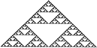
Figure 1: Evolution of CA given by rule number $90$. In this case, the initial configuratio is a finite one-dimensional lattice which has only one site with the value $1$ (pictured in black). Source: www.stephenwolfram.com/publications/articles/ca/

Once $r=1$ in expression (2), it is easy to check that this rule is defined by the function:

$$\begin{array}[]{lll}1&1&1\\ &0&\end{array}\quad\begin{array}[]{lll}1&1&0\\ &1&\end{array}\quad\begin{array}[]{lll}1&0&1\\ &0&\end{array}\quad\begin{array}[]{lll}1&0&0\\ &1&\end{array}\begin{array}[]{lll}0&1&1\\ &1&\end{array}\quad\begin{array}[]{lll}0&1&0\\ &0&\end{array}\quad\begin{array}[]{lll}0&0&1\\ &1&\end{array}\quad\begin{array}[]{lll}0&0&0\\ &0&\end{array}$$ (5)

$$0\ast 2^{7}+1\ast 2^{6}+0\ast 2^{7}+1\ast 2^{4}+1\ast 2^{3}+0\ast 2^{2}+1\ast 2^{1}+0\ast 2^{0}=90$$ (6)

By observing this example, we see that there are $2^{8}=256$ such rules and for each one it can be assigned a rule number following the indexation illustrated on expression 6. In [41], Wolfram proposes four basic classes of behavior for these rules (see also [3]):

Class 1: Evolution leads to homogeneous state in which all the sites have the same value (Figure 2.a);

Class 2: Evolution leads to a set of stable and periodic structures that are separated and simple (Figure 2.b);

Class 3: Evolution leads to a chaotic pattern (Figure 2.c);

Class 3: Evolution leads to complex structures (Figure 2.d).

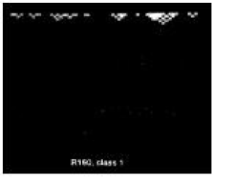
(a)

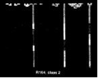
(b)

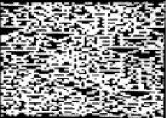
(c)

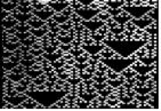
(d)

Figure 2: Some examples of Wolfram’s classification for one-dimensional $r=1$ CAs. Source: www.stephenwolfram.com/publications/articles/ca/

Other classifications based on Markovian processes and group properties can be also found in the literature [21, 11].

Despite of its local simplicity, knowledge discovery in CA is a NP problem. In fact, let us take a one-dimensional CA with a finite lattice $L$ of size $d$. One may consider the question of whether a particular sequence of $d$ site values can occur after $T$ time steps in the evolution of the cellular automaton, starting from any initial state. Then, one may ask whether there exists any algorithm that can determine the answer in a time given by some polynomial in $d$ and $T$. The question can certainly be answered by testing all sequences of possible initial site values, that is $(\#S)^{d}$. But this procedure requires a time that grows exponentially with $d$.

Nevertheless, if an initial sequence could be guessed, then it could be tested in a time polynomial in $d$ and $T$. As a consequence, the problem is in the class NP which motivates the application of data mining techniques for knowledge discovery in CA. The next sections review PCA basic theory and its application for the analysis of the (traditional) set of rules composed by $256$ $1D$ cellular automata obtained when $r=1$, $S=\left\{0,1\right\}$.

3 . Principal Component Analysis

Principal Component Analysis (PCA), also called Karhunen-Loeve, or KL method, can be seen as a method for data compression or dimensionality reduction [4] (see [27], section $5.11$ also). Thus, let us suppose that the data to be compressed consist of $N$ tuples or data vectors, from a n-dimensional space. Then, PCA searches for $k$ n-dimensional orthonormal vectors that can best be used to represent the data, where $k\leq n$. Figure 3.a,b picture this idea using a bidimensional representation. If we suppose the the data points are distributed over the elipse, it follows that the coordinate system ($\left(\overline{X},\overline{Y}\right)$, shown in Figure 3.b is more suitable for representing the data set in a sense that will be formally described next.

Thus, let $S=\left\{\mathbf{u}_{1},\mathbf{u}_{2},...,\mathbf{u}_{N}\right\}$ the data set represented on Figure 3. By now, let us suppose that the centroid of the data set is the center of the coordinate system, that means:

$$C_{M}=\frac{1}{N}\sum_{i=1}^{N}\mathbf{u}_{i}=\mathbf{0}.$$ (7)

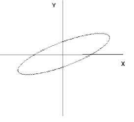
(a)

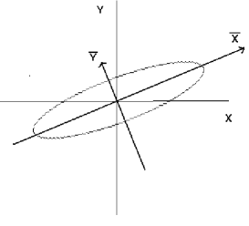
(b)

Figure 3: (a)Original dataset. (b) Extraction of the principal component.

To address the issue of compression, we need a vector basis that satisfies a proper optimization criterium (rotated axes in Figure 3.b). Following [27], consider the operations in Figure 4. The vector $\mathbf{u}_{j}$ is first transformed to a vector $\mathbf{v}_{j}$ by the matrix (transformation) $A$. Thus, we truncate $\mathbf{v}_{j}$ by choosing the first $m$ elements of $\mathbf{v}_{j}$. The obtained vector $\mathbf{w}_{j}$ is just the transformation of $\mathbf{v}_{j}$ by $I_{m}$, that is a matrix with 1s along the first $m$ diagonal elements and zeros elsewhere. Finally, $\mathbf{w}_{j}$ is transformed to $\mathbf{z}_{j}$ by the matrix $B$. Let the square error defined as follows:

$$J_{m}=\frac{1}{N}\sum_{j=0}^{N}\left\|\mathbf{u}_{j}-\mathbf{z}_{j}\right\|^{2}=\frac{1}{n}Tr\left[\sum_{j=0}^{N}\left(\mathbf{u}_{j}-\mathbf{z}_{j}\right)\left(\mathbf{u}_{j}-\mathbf{z}_{j}\right)^{*T}\right],$$ (8)

where $Tr$ means the trace of the matrix between the square brackets and the notation ($*T$) means the transpose of the complex conjugate of a matrix. Following Figure 4, we observe that $\mathbf{z}_{j}=BI_{m}A\mathbf{u}_{j}$. Thus we can rewrite (8) as:

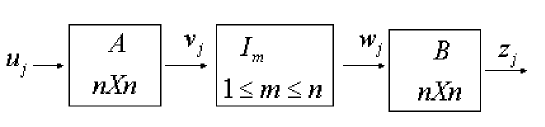
Figure 4: KL Transform formulation. Reprinted from [27].

$$J_{m}=\frac{1}{N}Tr\left[\sum_{i=0}^{N}\left(\mathbf{u}_{j}-BI_{m}A\mathbf{u}_{j}\right)\left(\mathbf{u}_{j}-BI_{m}A\mathbf{u}_{j}\right)^{*T}\right],$$ (9)

which yields:

$$J_{m}=\frac{1}{N}Tr\left[\left(I-BI_{m}A\right)R\left(I-BI_{m}A\right)^{*T}\right],$$ (10)

where:

$$R=\sum_{i=0}^{N}\mathbf{u}_{j}\mathbf{u}_{j}^{*T}.$$ (11)

Following the literature, we call $R$ the covariance matrix. We can now stating the optimization problem by saying that we want to find out the matrices $A,B$ that minimizes $J_{m}$. The next theorem gives the solution for this problem.

Theorem 1: The error $J_{m}$ in expression (10) is minimum when

$$A=\Phi^{*T},\quad B=\Phi,\quad AB=BA=I,$$ (12)

where $\Phi$ is the matrix obtained by the orthonormalized eigenvectors of $R$ arranged according to the decreasing order of its eigenvalues.

Proof. To minimize $J_{m}$ we first observe that $J_{m}$ must be zero if $m=n.$ Thus, the only possibility would be

$$I=BA\Rightarrow A=B^{-1}.$$ (13)

Besides, by remembering that

$$Tr\left(CD\right)=Tr\left(DC\right),$$ (14)

we can also write:

$$J_{m}=\frac{1}{n}Tr\left[\left(I-BI_{m}A\right)^{*T}\left(I-BI_{m}A\right)R\right].$$ (15)

Again, this expression must be null if $m=n$. Thus:

$$J_{n}=\frac{1}{n}Tr\left[\left(I-BA-A^{*T}B^{*T}+A^{*T}B^{*T}BA\right)R\right].$$

This error is minimum if:

$$B^{*T}B=I,\quad A^{*T}A=I,$$ (16)

that is, if $A$ and $B$ are unitary matrix. The next condition comes from the differentiation of $J_{m}$ respect to the elements of $A$. We should set the result to zero in order to obtain the necessary condition to minimize $J_{m}$. This yields:

$$I_{m}A^{*T}\left(I-A^{*T}I_{m}A\right)R=0,$$ (17)

which renders:

$$J_{m}=\frac{1}{n}Tr\left[\left(I-A^{*T}I_{m}A\right)R\right].$$ (18)

By using the property (14), the last expression can be rewritten as

$$J_{m}=\frac{1}{n}Tr\left[R-I_{m}ARA^{*T}\right].$$

Since $R$ is fixed, $J_{m}$ will be minimized if

$$\overset{\char 126\relax}{J}_{m}=Tr\left[I_{m}ARA^{*T}\right]=\sum_{i=0}^{m-1}a_{i}^{T}Ra_{i}^{*},$$ (19)

is maximized where $a_{i}^{T}$ is the ith row of $A$. Once $A$ is unitary, we must impose the constrain:

$$a_{i}^{T}a_{i}^{*}=1.$$ (20)

Thus, we shall maximize $\overset{\char 126\relax}{J}_{m}$ subjected to the last condition. The Lagrangian has the form:

$$\overset{\char 126\relax}{J}_{m}=\sum_{i=0}^{m-1}a_{i}^{T}Ra_{i}^{*}+\sum_{i=0}^{m-1}\lambda_{i}\left(1-a_{i}^{T}a_{i}^{*}\right),$$

where the $\lambda_{i}$ are the Lagrangian multipliers. By differentiating this expression respect to $a_{i}$ we get:

$$Ra_{i}^{*}=\lambda_{i}a_{i}^{*},$$ (21)

Thus, $a_{i}^{*}$ are orthonormalized eigenvectors of $R$. Substituting this result in expression (19) produces:

$$\overset{\char 126\relax}{J}_{m}=\sum_{i=0}^{m-1}\lambda_{i},$$ (22)

which is maximized if $\left\{a_{i}^{*},\quad i=0,1,...,m-1\right\}$ correspond to the largest eigenvalues of $R$. ($\square$)

A straightforward variation of the above statement is obtained if we have a random vector $\mathbf{u}$ with zero mean. In this case, the pipeline of Figure 4 yields a random vector $\mathbf{z}$ and the square error can be expressed as:

$$J_{m}=\frac{1}{n}Tr\left[E\left\{\left(\mathbf{u}-BI_{m}A\mathbf{u}\right)\left(\mathbf{u}-BI_{m}A\mathbf{u}\right)^{*T}\right\}\right],$$

which can be written as:

$$J_{m}=\frac{1}{n}Tr\left[\left(I-BI_{m}A\right)R\left(I-BI_{m}A\right)^{*T}\right],$$ (23)

where $R=E\left(\mathbf{uu}^{*T}\right)$ is the covariance matrix. Besides, if $C_{m}$ in expression (7) is not zero, we must translate the coordinate system to $C_{m}$ before computing the matrix $R$ , that is:

$$\widetilde{\mathbf{u}_{j}}=\mathbf{u}_{j}\mathbf{-C}_{m}.$$ (24)

In this case, matrix $R$ will be given by:

$$R=\sum_{i=0}^{N}\widetilde{\mathbf{u}_{j}}\widetilde{\mathbf{u}_{j}}^{*T}.$$

Also, sometimes may be useful to consider in expression (8) some other norm, not necessarily the 2-norm. In this case, there will be a real, symmetric and positive-defined matrix $M$, that defines the norm. Thus, the square error $J_{m}$ will be rewritten in more general form:

$$J_{m}=\frac{1}{n}\sum_{j=0}^{N}\left\|\mathbf{u}_{j}-\mathbf{z}_{j}\right\|_{M}^{2}=\frac{1}{n}\sum_{j=0}^{N}\left(\mathbf{u}_{j}-\mathbf{z}_{j}\right)^{*T}M\left(\mathbf{u}_{j}-\mathbf{z}_{j}\right).$$ (25)

Obviously, if $M=I$ we recover expression (8). The link between this case and the above one is easily obtained by observing that there is non-singular and real matrix $W$, such that:

$$W^{T}MW=I.$$ (26)

The matrix $W$ defines the transformation:

$$W\widehat{\mathbf{u}_{j}}=\mathbf{u}_{j},\quad W\widehat{\mathbf{z}_{j}}=\mathbf{z}_{j}.$$ (27)

Thus, by inserting these expressions in equation (25) we obtain:

$$J_{m}=\frac{1}{n}\sum_{j=0}^{N}\left(\widehat{\mathbf{u}_{j}}-\widehat{\mathbf{z}_{j}}\right)^{*T}\left(\widehat{\mathbf{u}_{j}}-\widehat{\mathbf{z}_{j}}\right).$$ (28)

Expression (28) can be written as:

$$J_{m}=\frac{1}{n}\sum_{j=0}^{N}\left\|\widehat{\mathbf{u}_{j}}-\widehat{\mathbf{z}_{j}}\right\|^{2},$$ (29)

now using the 2-norm, like in expression (8). Therefore:

$$J_{m}=\frac{1}{n}Tr\left[\sum_{j=0}^{N}\left(\widehat{\mathbf{u}_{j}}-\widehat{\mathbf{z}_{j}}\right)\cdot\left(\widehat{\mathbf{u}_{j}}-\widehat{\mathbf{z}_{j}}\right)^{*T}\right].$$ (30)

Following the same development performed above, we will find that we must solve the equation:

$$\widehat{R}\widehat{a_{i}^{*}}=\lambda_{i}\widehat{a_{i}^{*}},$$ (31)

where:

$$\widehat{R}=\sum_{j=0}^{N}\widehat{\mathbf{u}_{j}}\widehat{\mathbf{u}_{j}}^{*T}.$$ (32)

Thus, from transformations (27) it follows that:

$$\widehat{R}=WRW^{T}.$$ (33)

and, therefore, we must solve the following eigenvalue/eigenvector problem:

$$\left(WRW^{T}\right)\widehat{a_{i}^{*}}=\lambda_{i}\widehat{a_{i}^{*}}.$$ (34)

The eigenvectors, in the original coordinate system, are finally given by:

$$W\widehat{a_{i}^{*}}=a_{i}^{*}.$$ (35)

The next section shows the application of PCA method for knowledge discovery in CAs.

4 . PCA and Cellular Automata

In this section we review the work presented in [14]. In this reference, authors analyzed one-dimensional CAs using PCA. The key idea is to consider binary patterns of a pre-defined size $l$ as inputs of the CAs. It is considered the $256$ one-dimensional CA rules obtained for $r=1$ and $S=\left\{0,1\right\}$ in expression 1-2. The output can be collected in a Table, like Table 1, built for $l=5$.

Patterns	$R_{0}$	$R_{1}$	…	$R_{254}$	$R_{255}$
$00000$	$000$	$111$	…	$000$	$111$
$00001$	$000$	$110$	…	$001$	$111$
…	…	…	…	…	…
$11110$	$000$	$000$	…	$111$	$111$
$11111$	$000$	$000$	…	$111$	$111$

Table 1: Table which rows are indexed by binary patterns and collumns by the CA rules $R_{0}$, $R_{1}$, …, $R_{255}$.

Each row $j$ of Table 1 is obtained through the application of the rule $R_{j}$ (see expression 6 for an example of rule indexation) Then, I/0 patterns are converted to cardinal numbers denoted by $f_{j}\left(m_{i}\right)$, which means the cardinal number corresponding to the application of the rule $j$ to the pattern $i$ ($i=0,1,...,31$ for Table 1). Thus, in general we get the matrix:

$$F=\left[\begin{array}[]{ccc}f_{11}&\ldots&f_{1p}\\ \vdots&\ddots&\vdots\\ f_{n1}&\ldots&f_{np}\end{array}\right],$$ (36)

where $f_{ij}=f_{j}\left(m_{i}\right).$ The matrix $F$ is the data set to be analyzed..

For mining knowledge in $F$ through PCA we should firstly to perform the operation (translation) given by (24). Thus, matrix $F$ is converted to the following one:

$$X=\left[\begin{array}[]{ccc}x_{11}&\ldots&x_{1p}\\ \vdots&\ddots&\vdots\\ x_{n1}&\ldots&x_{np}\end{array}\right],$$ (37)

with:

$$x_{ij}=f_{j}(m_{i})-E_{j},$$ (38)

$$E_{j}=\frac{1}{n}\sum_{i=1}^{n}f_{j}(m_{i}).$$ (39)

The matrix $X$ is of size $np$. In [14] columns $x_{1},\ldots,x_{p}$ of $X$ are called variables while rows $e_{1},\ldots,e_{n}$ are called covariables. However, we must observe that space dimension is the number of rules $(p)$ and the number of data vectors is the number of patters $\left(n\right).$ Thus, following section 3, we should apply the PCA over the data set given by matrix $X^{T}$ in order to find out the principal components of the covariables space. Besides, in [14] the norm in the covariables space is defined by:

$$M=diag\left(\frac{1}{S_{1}^{2}},\frac{1}{S_{2}^{2}},...,\frac{1}{S_{p}^{2}}\right),$$ (40)

with:

$$S_{j}^{2}=\frac{1}{n^{2}}\left(n\sum_{i=1}^{n}x_{ij}^{2}-\left(\sum_{i=1}^{n}x_{ij}\right)^{2}\right)=\frac{1}{n}\sum_{i=1}^{n}\left(x_{ij}-E_{j}\right)^{2}.$$ (41)

Following section 3, we must solve equation (34) to find the eigenvalues and then apply expression (35) to get the eigenvectors in the desired representation. The Table 2 shows the largest eigenvalues of this matrix for the listed pattern sizes.

l	$\lambda_{1}$	$\lambda_{2}$	$\lambda_{3}$	$\lambda_{4}$	$\lambda_{5}$	$\lambda_{6}$	$\lambda_{7}$
4	52.6802	48.2214	36.8869	36.8263	36.3134	24.4539	18.6179
5	58.2575	50.9776	37.2301	37.0399	30.7382	21.7355	18.0214
6	59.5952	51.6519	37.3406	37.1109	29.3769	21.0940	17.8305
7	59.9260	51.8197	37.3696	37.1296	29.0383	20.9358	17.7811
9	60.0290	51.8721	37.3788	37.1355	28.9325	20.8865	17.7656
12	60.0358	51.8755	37.3794	37.1359	28.9256	20.8833	17.7645

Table 2: Eigenvalues of the correlation matrix.

The main result is that the eigenvalues from the seventh rank are dramatically smaller in magnitude ($104$ times) than the first seven ones. Such observation led authors of [14] towards the following conjecture:

Conjecture: The rank of $R$ is $7$ and does not depend on the size $l$ of patterns being considered. When $l$ is increased the eigenvalues tend to characteristic values obtained for $l=12.$

This is the main result presented in [14]. Next, we show our results by applying the same analysis but introducing randomness in the CA behavior.

5 . PCA and Probabilistic Cellular Automata

In this section we report some experimental results obtained in the presence of noise which randomly reverses the CA output values with probability $p$. In the first experiment, reported on Table 3, we set $l=5$ and take some values for the probability $p$ and compute the PCA for the generated matrix.

	P=0.2	P=0.4	P=0.6	P=0.8
$\lambda_{1}$	30.993277	14.347278	27.368784	28.491445
$\lambda_{2}$	17.127385	13.29037	16.960658	17.279648
$\lambda_{3}$	13.541144	12.885112	14.959948	14.604408
$\lambda_{4}$	13.180114	11.816202	13.281494	13.752977
$\lambda_{5}$	12.388441	11.678309	11.357819	12.844465
$\lambda_{6}$	10.902415	11.37782	10.857413	10.829726
$\lambda_{7}$	10.293973	11.020907	9.959074	9.7779532
$\lambda_{8}$	9.90735	10.419589	9.5077103	9.2701578
$\lambda_{9}$	9.2822227	10.270046	9.3582306	8.8721786
$\lambda_{10}$	8.7295329	9.8165154	8.8984414	8.8107682
$\lambda_{11}$	8.529595	9.2160415	8.5837995	8.2016704
$\lambda_{12}$	7.8843864	8.9368721	8.3232351	8.0601548
$\lambda_{13}$	7.6179283	8.8871718	8.1230224	7.6299203
$\lambda_{14}$	7.0733465	8.4223863	7.8908832	7.5448918
$\lambda_{15}$	6.8634222	8.2353647	7.401953	7.3142038
$\lambda_{16}$	6.7723605	7.9216589	7.2366057	7.066622
$\lambda_{17}$	6.4657069	7.4769038	6.6688247	6.635226
$\lambda_{18}$	6.3216585	7.0701685	6.190632	6.1886655
$\lambda_{19}$	6.1603787	6.7891207	6.1204134	6.0738189
$\lambda_{20}$	5.8044919	6.6787658	5.7734589	5.8293511
$\lambda_{21}$	5.6959129	6.2790179	5.7684386	5.5555388
$\lambda_{22}$	5.3941432	6.0714589	5.2569218	5.472738
$\lambda_{23}$	4.9930157	5.8968197	4.9528161	5.2651065
$\lambda_{24}$	4.799646	5.6406084	4.7506673	4.896581
$\lambda_{25}$	4.5991479	5.5455414	4.5796108	4.7932072
$\lambda_{26}$	4.3609133	5.2887732	4.5370786	4.7514249
$\lambda_{27}$	4.1529641	5.1079093	4.3017415	4.2932052
$\lambda_{28}$	3.9754383	4.9468391	4.0258767	3.7535244
$\lambda_{29}$	3.7421531	4.826271	3.850906	3.6713829
$\lambda_{30}$	3.3309643	4.362729	3.7734524	3.4443371
$\lambda_{31}$	3.1165726	3.4774291	3.3800895	3.0247033
$\lambda_{32}$	7.075E-15	5.587E-15	5.641E-15	7.235E-15

Table 3: Principal components for patterns with $l=5$ and noise with probability distribution given by $p$.

We observe that the number of principal components is $31$ for all tests. When size patterns are increased to ($l=6,7,9,12$) we observe (see Tables 4 and 5 for $l=6$ ) the same behavior but the number of principal components increases to $63,127,254,254,$ respectively. In these tests, for a fixed pattern size, the noise intensity ($p$ value) did not seem to play a considerable effect in the number of principal components if $p>0.2$. However if $p=0.0$, we know from the conjecture of section 4 that this number is $7$ for all cases considered. What happens for $0.0<p<0.2$?

Such question must be considered in further works by the viewpoint of the KL transform, following the procedure of section 3 for a random field $\mathbf{u}\left(i,j\right)$ in order to have a complete answer.

	P=0.2	P=0.4	P=0.6	P=0.8
$\lambda{1}$	25.490674	9.0159666	25.916423	26.284694
$\lambda{2}$	14.10028	8.5855201	14.41566	14.102228
$\lambda{3}$	11.104733	7.9801912	10.70382	10.688536
$\lambda{4}$	10.790121	7.7267394	10.065372	9.7791048
$\lambda{5}$	9.0958191	7.4831015	9.6810207	9.1538961
$\lambda{6}$	7.2510569	7.3765707	7.638434	6.6054597
$\lambda{7}$	6.8531309	7.0389042	6.8077442	6.4860439
$\lambda{8}$	6.286914	6.9484678	6.2549327	6.1013626
$\lambda{9}$	6.1443606	6.6158667	6.121154	5.9897572
$\lambda{10}$	5.8704541	6.4728947	5.8079843	5.7110224
$\lambda{11}$	5.6239779	6.3245388	5.6570288	5.3881715
$\lambda{12}$	5.4920906	6.1992113	5.3781214	5.3309815
$\lambda{13}$	5.2459503	5.9229922	5.2887514	5.1818583
$\lambda{14}$	5.0507806	5.7271535	5.0157005	5.0733092
$\lambda{15}$	4.8419224	5.5844553	4.9008587	4.9569268
$\lambda{16}$	4.7432239	5.4868919	4.7443148	4.9045772
$\lambda{17}$	4.5913664	5.4394466	4.646143	4.8375055
$\lambda{18}$	4.5541085	5.2349427	4.519477	4.6544779
$\lambda{19}$	4.3368357	5.1286	4.4405929	4.3767439
$\lambda{20}$	4.289522	5.0877569	4.3612835	4.255288
$\lambda{21}$	4.0221739	4.8696669	4.1463912	4.1147127
$\lambda{22}$	4.0053207	4.7376638	4.0277528	3.9599816
$\lambda{23}$	3.9195876	4.6631356	3.9294454	3.8759049
$\lambda{24}$	3.8132963	4.5676061	3.8562459	3.7592389
$\lambda{25}$	3.6929406	4.5192326	3.7291963	3.6175464
$\lambda{26}$	3.6059328	4.3866647	3.6566283	3.5898727
$\lambda{27}$	3.5245448	4.2816878	3.4551909	3.4851947
$\lambda{28}$	3.4689985	4.1503676	3.4185097	3.4233569
$\lambda{29}$	3.3229986	4.0343815	3.2894165	3.376657
$\lambda{30}$	3.2214124	3.905456	3.2094177	3.247659
$\lambda{31}$	3.1659706	3.7940953	3.1942609	3.2206595

Table 4: The first $31$ principal components for patterns with $l=6$ and noise with probability distribution given by $p$.

	P=0.2	P=0.4	P=0.6	P=0.8
$\lambda{32}$	3.1278811	3.6850001	3.0605835	3.1566209
$\lambda{33}$	2.9093472	3.5911018	2.9959418	2.9694106
$\lambda{34}$	2.8851128	3.4984597	2.903988	2.9241726
$\lambda{35}$	2.8361213	3.3609776	2.8339349	2.9066998
$\lambda{36}$	2.7116889	3.2629616	2.7802321	2.8511868
$\lambda{37}$	2.6410113	3.1449082	2.7448714	2.7909378
$\lambda{38}$	2.62132	3.1060263	2.5446362	2.6124111
$\lambda{39}$	2.5625247	3.0036165	2.4679447	2.591938
$\lambda{40}$	2.4466011	2.9296411	2.4130114	2.5655322
$\lambda{41}$	2.3957291	2.7868727	2.3229128	2.4194093
$\lambda{42}$	2.3022031	2.729422	2.2821061	2.3069397
$\lambda{43}$	2.1920726	2.717123	2.1595839	2.2493672
$\lambda{44}$	2.1758946	2.603908	2.1373086	2.1920309
$\lambda{45}$	2.0950959	2.4974377	2.0678771	2.1697002
$\lambda{46}$	2.0489445	2.3755221	1.9724868	2.0876546
$\lambda{47}$	2.020732	2.3495888	1.9516421	2.0184278
$\lambda{48}$	1.9777077	2.2768661	1.8642426	1.9885042
$\lambda{49}$	1.8766222	2.1822128	1.8066548	1.8790247
$\lambda{50}$	1.7943956	2.1355595	1.758534	1.8591266
$\lambda{51}$	1.7171865	2.0430028	1.6877656	1.7836542
$\lambda{52}$	1.6253386	2.022733	1.6355071	1.6965591
$\lambda{53}$	1.5259488	1.9193735	1.6129515	1.6380111
$\lambda{54}$	1.4965356	1.807634	1.4445091	1.5871297
$\lambda{55}$	1.4114911	1.7544899	1.3778514	1.5641227
$\lambda{56}$	1.381066	1.7005373	1.3387275	1.5194184
$\lambda{57}$	1.3691854	1.6217295	1.2709127	1.3652494
$\lambda{58}$	1.2926625	1.4695063	1.2284464	1.2780083
$\lambda{59}$	1.1645091	1.4539369	1.1474655	1.2135036
$\lambda{60}$	1.1101623	1.3227765	1.1182555	1.1747427
$\lambda{61}$	0.9979225	1.1870755	1.0455127	1.120168
$\lambda{62}$	0.9866537	1.1730686	0.9469073	1.0335351
$\lambda{63}$	0.7798336	0.9967607	0.7994225	0.9540748
$\lambda{64}$	4.890E-15	3.123E-15	8.151E-15	6.998E-15

Table 5: The last $33$ principal components for patterns with $l=6$ and noise with probability distribution given by $p$.

However, an interesting points is that these question resemble the problem of studying the influence of control parameters in continuous dynamical systems [23]. With such parameters we can control the influence of factors like temperature, viscosity, irradiation, etc. Those systems can be analyzed through stability analysis [26, 23], bifurcation and catastrophe theory [26, 1] and perturbation [23]. In that context, there may be critical values for the parameters, in the sense that sudden changes happen near them. As an example, let us consider a simple dynamical system:

$$\frac{dx}{dt} = \lambda x+y$$ (42)

$$\frac{dy}{dt} = x+\lambda y$$

where $\lambda$ is a real parameter. According to the theory of ordinary differential equations [23], the qualitative analysis of this system may be done through the analysis of the eigenvalues/eigenvectors of the matrix of the above system:

$$A=\left[\begin{array}[]{ll}\lambda&1\\ 1&\lambda\end{array}\right].$$ (43)

The eigenvalues are given by:

$$\alpha_{1}=\lambda+1,\quad\alpha_{2}=\lambda-1.$$ (44)

We observe that the value $\lambda=1$ is a critical one because, for $\lambda>1$ the origin $\left(0,0\right)$ is an attractor but for $\lambda<1$ we observe a saddle point. Thus, we have a jump, that is, a sudden change in the system behavior, for $\lambda=1.$

Cellular automata are discrete dynamical systems for which the probability $p$ could be seem as a parameter that ranges in $\left[0,1\right]$. Would there be critical values in this case? If the answer is ”yes” which property suddenly changes? Could it be the number of principal components?

These questions and the mathematical theory necessary to perform such analysis are points that we shall consider in further works.

6 . Final Comments

In this paper we review the application of PCA for cellular automata analysis. We follow the work presented in [14] but in the presence of noise which randomly reverses the CA output values with probability $p$. We observe that, for a fixed pattern size, the noise intensity ($p$ value) did not seem to play a considerable effect in the number of principal components if $p>0.2$. The observed (and expected) influence is that the number of principal components increases. For example, if $l=5$ and $p=0.0$, the main result of [14] says that this number is $7$ while for $p\in\left\{0.2,0.6,0.8\right\}$ this number increases to $31$. The obvious question is that what happens for $0.0<p<0.2$?

This and others questions about parameter sensitivity analysis for cellular automata must be answered in further works.

7 .  Acknowledgments

We would like to acknowledge CNPq for the financial support for this work.

References

- [1] Catastrophe Theory and Its Application. London Pitman publishing, 1978.
- [2] A new kind of science. Wolfram Media Inc., Champaign, Ilinois, US, United States, 2002.
- [3] C. Adami. Introduction to Artificial Life. Springer, New York, 1998.
- [4] V. Algazi and D. Sakrison. On the optimality of karhunen-loeve expansion. IEEE Trans. Information Theory, pages 319–321, 1969.
- [5] C. Bays. Patterns for simple cellular automata in a universe of dense packed spheres. Complex Systems, 1(6):853–875, Dec. 1987.
- [6] N. Boccara, J. Nasser, and M. Roger. Particle-like structures and interactions in spatio-temporal patterns generated by one-dimensional deterministic cellular automaton rules. Phys. Rev. A, 44, July 1991.
- [7] P. Chaudhuri, D. Chowdhury, S. Nandi, and S. Chatterjee. Additive Cellular Automata, Theory and Applications, volume 1. IEEE Computer Society Press, Los Alamitos, California, 1997.
- [8] B. Chopard and M. Droz. Cellular Automata Modeling of Physical Systems. Cambridge University Press, 1998.
- [9] B. Chopard, A. Dupuis, A. Masselot, and P. Luthi. Cellular automata and lattice boltzmann techniques: An approach to model and simulate complex systems. Advances in complex systems, 5(2):1–144, 2002. special issue on: Applications of Cellular Automata in Complex Systems.
- [10] A. K. Das and P. P. Chaudhuri. Vector space theoretic analysis of additive cellular automata and its application for pseudoexhaustive test pattern generation. IEEE Trans. Comput., 42(3):340–352, 1993.
- [11] A. K. Das, A. Sanyal, and P. Palchaudhuri. On characterization of cellular automata with matrix algebra. Inf. Sci., 61(3):251–277, 1992.
- [12] J. Demongeot, E. Goles, and M. Tchuente, editors. Dynamical Systems and Cellular Automata, Proceedings of the Conference on Dynamical Behaviour of Cellular Automata: Theory and Applications, Luminy, France, September 13–17, 1983. Academic Press, London.
- [13] J. Demongeot, E. Goles, and M. Tchuente. Dynamical systems and cellular automata. Academic Press, New York, 1985.
- [14] L. Deniau and J. Blanc-Talon. PCA and cellular automata: a statistical approach for determnistic machines. 1994.
- [15] G. B. Ermentrout and L. Edelstein-Keshet. Cellular automata approaches to biological modeling. J. theor. Biol., 160:97–133, 1993.
- [16] G. B. Ermentrout and L. Edelstein-Keshet. Cellular automata approaches to biological modeling. Journal of Theoretical Biology, 160:97–133, Jan 1993.
- [17] H. Fang, Z. Wang, Z. Lin, and M. Liu. Lattice boltzmann method for simulating the viscous flow in large distensible blood vessels. Physical Review E, 65:051925, 2002.
- [18] I. M. Group. Cam8: a parallel, uniform, scalable architecture for ca experimentation. http://www.im.lcs.mit.edu/cam8.
- [19] H. Gutowitz. Statistical properties of cellular automata in the context of learning and recognition. part i: Introduction. In K. Zhao, editor, Learning and Recognition–A Modern Approach, pages 233–255. World Scientific Publishing, Singapore, 1989.
- [20] H. Gutowitz. Statistical properties of cellular automata in the context of learning and recognition. part II: Inverting local structure theory equations to find cellular automata with specified properties. In K. H. Zhao, editor, Learning and Recognition–A Modern Approach, pages 256–280. World Scientific Publishing, Singapore, 1989.
- [21] H. Gutowitz. A hierarchical classification of CA. Physica D, 45:136, 1990.
- [22] H. Gutowitz. A massively parallel cryptosystem based on cellular automata. In B. Schneier, editor, Applied Cryptography. K. Reidel, 1993.
- [23] H. Haken. Advanced Synergetics: Instability Hierarchies of Self-Organizing Systems and Devices. Springer-Verlag, New York, 1987.
- [24] J. Han and M. Kamber. Data Mining: Concepts and Techniques. The Morgan Kaufmann Series in data man. syst., 2001.
- [25] H. Hartman and G. Vichniac. Inhomogenous cellular automata. In E. Bienenstock and et al., editors, Disordered Systems and Biological Organization. unknown, 1900.
- [26] G. Iooss and D. Joseph. Elementary Stability and Bifurcation Theory. Springer-Verlag, New York, 1997.
- [27] A. K. Jain. Fundamentals of Digital Image Processing. Prentice-Hall, Inc., 1989.
- [28] L. Kadanoff, G. McNamara, and G. Zanetti. From automata to fluid flow: Comparisons of simulation and theory. Physical Review A, 40(8):4527–4541, 89.
- [29] O. Martin, A. Odlyzko, and S. Wolfram. Algebraic properties of cellular automata. Commun. Math. Phys., 93:219, 1984.
- [30] F. J. Morales, J. Crutchfield, and M. Mitchell. Evolving two-dimensional cellular automata to perform density classification: a report on work in progress. In S. B. et al., editor, Cellular automata: research towards industry, pages 3–14. Springer-Verlag, 1998.
- [31] J. V. Neumann. The Theory of Self-Reproducing Automata. Ed. Urbana, IL: Univ. Illinois Press, 1966.
- [32] J. Pedersen. Cellular automata as algebraic systems. Complex Systems, 6(3):237–250, June 1992.
- [33] A. Pires, D. Landau, and H. Herrmann, editors. Computational Physics and Cellular Automata. World Scientific, 1990.
- [34] P. Sarkar. A brief history of cellular automata. ACM Comput. Surv., 32(1):80–107, 2000.
- [35] L. S. Schulman and P. E. Seiden. Statistical mechanics of a dynamical system based on conway’s game of life. J. Stat Phys., 19:293, 1978.
- [36] H. B. Sieburg and O. K. Clay. Cellular automata as algebraic systems. Complex Systems, 5(6):575–602, Dec. 1991.
- [37] S. Succi. The Lattice Boltzmann Equation for Fluid Dynamics and Beyond (Numerical Mathematics and Scientific Computation). Oxford University Press, 2nd edition, 2002.
- [38] S. Wolfram. Web Site.
- [39] S. Wolfram. Statistical mechanics of cellular automata. Rev. Mod. Phys., 55:601–644, 1983.
- [40] S. Wolfram. Computational theory of cellular automata. Communications in Mathematical Physics, 96:15–57, 1984.
- [41] S. Wolfram. Universality and complexity in cellular automata. Physica D, 10:1–35, 1984.
- [42] S. Wolfram. Cellular automaton fluid: basic theory. J. Stat. Phys., 45:471, 1986.
- [43] S. Wolfram. Cellular Automata and Complexity. Addison-Wesley, Reading MA, 1994.