Non-coherent Rayleigh fading MIMO channels: Capacity Supremum

Abstract

This paper investigates the limits of information transfer over a fast Rayleigh fading MIMO channel, where neither the transmitter nor the receiver has the knowledge of the channel state information (CSI) except the fading statistics. We develop a scalar channel model due to absence of the phase information in non-coherent Rayleigh fading and derive a capacity supremum with the number of receive antennas at any signal to noise ratio (SNR) using Lagrange optimisation. Also, we conceptualise the discrete nature of the optimal input distribution by posing the optimisation on the channel mutual information for $N$ discrete inputs. Furthermore, we derive an expression for the asymptotic capacity when the input power is large, and compare with the existing capacity results when the receiver is equipped with a large number of antennas.

I Introduction

Communication over rapidly time-varying channels where the receiver is unable to estimate the channel state is a challenging task. In particular, for a mobile receiver the estimation may become difficult and the limits of information transfer in this scenario is vital when the channel becomes non-coherent. In this paper we study the capacity of the non-coherent Rayleigh fading MIMO channel to identify the limits of information transfer with no CSI at both ends.

One of the important problems in information theory is that of computing the capacity of a given communication channel, and finding the optimal input distribution that achieves capacity. The capacity problem is addressed by maximising the mutual information, a concave function subject to some constraints on the channel input distribution. For discrete finite-size input alphabets, this is a finite dimensional problem and all the input constraints are such that they define a compact, convex set, where the optimisation is straightforward. However, for continuous input channels, neither the continuity of the objective function, nor the compactness of the constraint set is now obvious, and the optimisation for capacity is considered a difficult problem [5, 8].

A large amount of literature has appeared in the area of multi-antenna wireless communications over the past decade. Much of the interest was motivated by the work in [1, 12] which shows a potential increase in the channel capacity using multiple antennas for both transmitting and receiving. The capacity of the MIMO channel, when neither the transmitter nor the receiver has CSI, has traditionally been considered an open and difficult problem. In this paper, we provide an upper bound on the non-coherent Rayleigh fading MIMO channel capacity for any receive antenna number at any SNR and elaborate on the discrete nature of the optimal input.

The MIMO channel capacity derived in [1], is based on the assumptions that i) the channel matrix elements are independent and circularly symmetric complex Gaussian; ii) the noise at different receive antennas are independent and white and; iii) the CSI is perfectly known at the receiver but not to the transmitter. The main result is linear capacity growth with the minimum number of transmit and receive antennas. Also [1] shows that the optimum input distribution which achieves this channel capacity is circularly symmetric complex Gaussian which maximises the channel output entropy when the CSI is known.

The capacity evaluation using Monte Carlo method when the receiver CSI is perfectly known is shown in [2]. The results extends Telatar’s work [1] and provides accurate numerical results. Furthermore [3] shows the use of water filling on the input Gaussian vector when receiver and transmitter CSI is available at the both transmitter and receiver. The increase in capacity is significant for small number of antennas and at low SNR. At high SNR the fading is less destructive and the water filling solution does not provide a considerable gain over the capacity with CSI at the receiver only.

The non-coherent channel capacity of the time selective Rayleigh fading channel is studied in [4]. Upper and lower bounds on the capacity at high SNR for single antenna systems is shown, and derived a lower bound on the capacity with multi-antennas. Abou-Faycal, Trott and Shamai [5] investigated the single input single output (SISO) discrete time memoryless Rayleigh fading channel, proving that the capacity achieving distribution is discrete with a finite number of mass points. In addition, Taricco [6] showed the capacity supremum and confirmed that the attainable input distribution is discrete in agreement with Abou-Faycal’s results. A general channel model is considered in [7] ignoring the structure of the channel.

Conversely in [8], the channel is assumed to have only additive noise, and in [5, 6], the channel is assumed to have both additive and multiplicative noise. In [7] it is shown that under a peak power constrained input, the capacity achieving input distribution is discrete, and attempts to make a case for the argument that continuous capacity achieving distributions are actually anomalies, and for most channels the optimal input distribution is discrete with a finite number of mass points.

Similar work is reported by Marzetta and Hochward [9] in non-coherent Rayleigh fading MIMO channels using a block fading model over a coherence interval of $T$ symbol periods. They characterised a certain structure of the optimal input distribution and computed the channel capacity with reduced complexity. The coherence capacity with channel coherence time $T$ is used as the upper bound.

Also, it is shown that the non-coherent channel capacity approaches the coherent capacity as $T$ becomes large where the optimal input is approximately independent complex Gaussian. Zheng and Tse [10] extended this work and specifically computed the asymptotic capacity at both high and low SNR in terms of $T$ and the number of transmit and receive antenna elements. The suggested input is to transmit orthogonal vectors on a certain number of transmit antennas with constant equal norms. They also claim that having more transmit antennas than receive antennas does not provide any capacity gain at high SNR, while having more receive antennas yield a capacity gain.

Recently, Lapidoth and Moser [11] showed the capacity of non-coherent multi antenna systems grows only double logarithmically in SNR and evaluated the fading number with the optimum input distributions in the high SNR region. This double logarithmic bahavior is a good example to visualise the low capacity available with no CSI compared to the coherent capacity given for MIMO [1, 12] and SISO [13] systems respectively.

In this paper we address the non-coherent uncorrelated Rayleigh fading MIMO channel and show a capacity supremum optimising the mutual information under average power constrained input for any SNR.

The contributions of the paper as follows:

1. We provide the mutual information of the non-coherent Rayleigh fading MIMO channel in simple form using output differential entropies.

2. We optimise the mutual information using Lagrange optimisation method and show a capacity supremum for a given number of receive antennas at any SNR.

3. We show the asymptotic analysis of the capacity supremum with double logarithmic behavior at high SNR, similar to the results shown in [11] and conjecture the discrete nature of the optimal input.

4. The proposed capacity in this paper can be taken as an upper bound to the non-coherent uncorrelated MIMO channel capacity in Rayleigh fading.

The organisation of this paper is as follows. Section II contains the channel model with notations used for the non-coherent Rayleigh fading MIMO communication system. The derivation of mutual information for the introduced channel model is presented in Section III, along with the detailed work based on Lagrange optimisation for channel capacity in IV. Section V presents the numerical results and analysis of our results. Finally conclusions are drawn in Section VI.

II MIMO Channel Model

The input output relationship of a MIMO channel can be written as

$$\boldsymbol{Y}={\boldsymbol{H}}{\boldsymbol{X}}+{\boldsymbol{N}},$$ (1)

where the output $\boldsymbol{Y}$ is $n_{r}\times 1$, the channel gain matrix $\boldsymbol{H}$ is $n_{r}\times n_{t}$. The input $\boldsymbol{X}$ is $n_{t}\times 1$ and the noise $\boldsymbol{N}$ which is assumed to be zero mean complex Gaussian is $n_{r}\times 1$. Each element of $\boldsymbol{H}$, $h_{{i}{j}},i=1,...,n_{r},j=1,...,n_{t}$ is assumed to be zero mean circular complex Gaussian random variables with a unit variance in each dimension.

We use $X=|\boldsymbol{X}|$ and $Y=|\boldsymbol{Y}|$ to denote the random scalar variables where $|\cdot|$ is the Euclidean norm. $x$ and $y$ represent each realisation of $X$ and $Y$ (i.e. $x\,\epsilon\,X$ and $y\,\epsilon\,Y$). The input is power limited with an average power constraint $\int{x^{2}}{p_{X}(x)}{d{x}}\leq P$. $n_{t}$ and $n_{r}$ denote the number of transmit and receive antennas respectively, and $\gamma=-\int_{0}^{\infty}{e^{-y}}{\log{y}}{dy}\,\approx 0.5772...,$  denotes the Euler’s constant. We use $\Gamma(\cdot)$ and $\Psi(\cdot)$ to indicate Gamma and Psi functions respectively. $h(\boldsymbol{X})$ denotes the differential entropy of $\boldsymbol{X}$, and $I(\boldsymbol{X};\boldsymbol{Y})$ designates the mutual information between $\boldsymbol{X}$ and $\boldsymbol{Y}$. The expected value over a set of random variables are denoted by $E\{\cdot\}$, with $\text{det}\,(\cdot)$ for the determinant, $(\cdot)^{*}$ for conjugate transpose of a matrix and $I$ for an identity matrix. All the differential entropies and the mutual information are defined to the base “e”, and the results are expressed in “nats”. Neither the receiver nor the transmitter has the knowledge of CSI except the fading statistics. Channel coherence time is one where the channel changes independently at every transmitted symbol.

III MIMO Mutual Information

III-A Capacity with Receiver CSI

The Rayleigh fading MIMO channel capacity when the receiver has the perfect CSI, given by,

$$C_{\text{rcsi}}=\mathrm{E}_{\boldsymbol{H}}\left[\log{\text{det}}\left(I_{n_{r}}+\frac{P}{n_{t}}{\boldsymbol{H}}{\boldsymbol{H}^{*}}\right)\right]$$ (2)

was derived by Telatar in optimising the mutual information $I(\boldsymbol{X};\boldsymbol{Y})=h(\boldsymbol{Y})-h(\boldsymbol{N})$ [1] and later Foschini [12] who extended the work to show how the capacity scales with increasing SNR for a large but practical number of antenna elements at both the transmitter and receiver. The linear growth of the capacity with $n_{r}$ is shown for a special case where the channel matrix $\boldsymbol{H}=I_{{n_{r}}{n_{t}}}$. The capacity increase in (2) is more prominent having multiple antennas at the receiver instead of the transmitter. However, under fast fading conditions, the estimation of fading coefficients which are assumed to be independent could be difficult due to the short duration of fades. It is of interest to study the capacity of such a channel and understand the ultimate limits when no CSI is available. Furthermore, the increasing demand for higher date rates along with mobility will make the instantaneous channel measurement more difficult. Therefore, it is important to find the optimal rate when the CSI is not perfectly available at the receiver (non-coherent). In this paper, we consider the mutual information of non-coherent uncorrelated Rayleigh fading MIMO channel and investigate the capacity.

III-B Mutual Information

The conditional probability density function (pdf) of the output given input of channel model (1) is given by

$$f_{\boldsymbol{Y}|\boldsymbol{X}}(y|x)=\frac{1}{(2{\pi}{(1+x^{2})})^{n_{r}}}{\exp\left[{-{\frac{y^{2}}{2{(1+x^{2})}}}}\right]},$$ (3)

where $f_{\boldsymbol{Y}|\boldsymbol{X}}(y|x)\triangleq\,f_{\boldsymbol{Y}|\boldsymbol{X}}(y_{1},y_{2},...,y_{n_{r}}|x_{1},x_{2},...,x_{n_{t}})$, $y\,\epsilon\,|\boldsymbol{Y}|$ and $x\,\epsilon\,|\boldsymbol{X}|$. The magnitude sign is removed in (3) for simplicity and likewise in the rest of this paper since the non-coherent Rayleigh fading channel does not carry any phase information [6]. The pdf of the magnitude distribution of (3) has the form

$$p_{Y|X}(y|x)=\frac{{y^{2{n_{r}}-1}}{\exp\left[{-{\frac{y^{2}}{2{(1+x^{2})}}}}\right]}}{{2^{n_{r}-1}}{\Gamma(n_{r})}{(1+x^{2})^{n_{r}}}}$$ (4)

when Jacobian coordinate transformation is applied on $2{n_{r}}$ dimensions. The output conditional entropy $h(\boldsymbol{Y}|\boldsymbol{X})$ for (1) is given by

$$h(\boldsymbol{Y}|\boldsymbol{X})=-\mathrm{E}_{x}\left\{{\int_{0}^{\infty}}{p_{Y|X}(y|x)}\,{\log\left[{p_{Y|X}(y|x)}\right]}{d{{y}}}\right\},$$ (5)

where the expectation is taken over $x\,\epsilon\,X$. With (4), we get

$$h(\boldsymbol{Y}|\boldsymbol{X}) =\frac{1}{2}{\mathrm{E}_{x}\left\{{\log(1+x^{2})}\right\}}+\log\left[\frac{\Gamma(n_{r})}{\sqrt{2}}\right]$$

$$-\left(n_{r}-\frac{1}{2}\right)\Psi(n_{r})+n_{r}.$$ (6)

Equation (6) can be used to calculate the output conditional entropy of uncorrelated Rayleigh fading MIMO channel when no CSI is available for a given input distribution. With the output entropy $h(\boldsymbol{Y})=-\int_{0}^{\infty}{p_{Y}(y)}{\log[p_{Y}(y)]}{dy}$, we obtain the mutual information [14]

$$I(\boldsymbol{X};\boldsymbol{Y}) =h(\boldsymbol{Y})-h(\boldsymbol{Y}|\boldsymbol{X})$$

$$=-\int_{0}^{\infty}{p_{Y}(y)}{\log\left[p_{Y}(y)\right]}{d{{y}}}-\frac{1}{2}{\mathrm{E}_{x}\left\{{\log(1+x^{2})}\right\}}$$

$$-\log\left[\frac{\Gamma(n_{r})}{\sqrt{2}}\right]+\left(n_{r}-\frac{1}{2}\right)\Psi(n_{r})-n_{r}.$$ (7)

From (7), the mutual information for a given input distribution can be computed. However, finding the optimal input and hence the capacity for a given input constraint is difficult. In next Section, we show how to derive un upper bound on (7) identifying some key properties of the optimal input.

IV Non-Coherent MIMO Capacity

IV-A Output Constraints

To obtain an expression for capacity of no-coherent Rayleigh fading MIMO channel, equation (7) needs to be maximised subject to an appropriate constraint on the input. Usual constraints used are $\int_{0}^{\infty}{p_{X}(x)}{d{{x}}}=1$ and $\int_{0}^{\infty}{{x}^{2}}{p_{X}(x)}{d{{x}}}=P$. However, the maximisation of (7) subject to these constraints does not provide a valid input pdf for SISO or MIMO in this case. To overcome this difficulty, additional constraints are used in [6] for SISO non-coherent Rayleigh fading channel. Likewise, to optimise (7) we use the following constraints

$$\int_{0}^{\infty}{p_{Y}(y)}{d{{y}}}=1,$$ (8a)

$$\int_{0}^{\infty}{{y}^{2}}{p_{Y}(y)}{d{{y}}}={2}{n_{r}}(1+P),$$ (8b)

$$\int_{0}^{\infty}{p_{Y}(y)}{\log{y}}{d{{y}}}=\frac{1}{2}{({\beta}+\Psi(n_{r})+\log{2})},$$ (8c)

where $\beta={\mathrm{E}_{x}\left\{{\log(1+x^{2})}\right\}}$. The second constraint is the average mean squared power of $y\,\epsilon\,Y$, which is considered as the induced power at the output by the input, channel gain and noise. The constraint (8c), is derived in Appendix VII-A. This additional constraint is used to support the optimisation process in order to arrive at a valid output pdf. Similar techniques are commonly employed in convex optimisation work [15].

IV-B Lagrange Optimisation

Using the Lagrange variable $L$ and the multipliers $\lambda_{1},\,\lambda_{2}$ and $\lambda_{3}$, we define

$$L =I(\boldsymbol{X};\boldsymbol{Y})+\lambda_{1}{\left[\int_{0}^{\infty}{p_{Y}(y)}{d{{y}}}-1\right]}$$

$$+\lambda_{2}\left[\int_{0}^{\infty}{{y}^{2}}{p_{Y}(y)}{d{{y}}}-{2}{n_{r}}(1+P)\right]$$

$$+\lambda_{3}\left[\int_{0}^{\infty}{p_{Y}(y)}{\log{y}}{d{{y}}}-\frac{1}{2}{({\beta}+\Psi(n_{r})+\log{2})}\right].$$ (9)

Solving (9) for $p_{Y}(y)$, we obtain the optimum output pdf

$$p_{Y}(y)={\exp\left[{(\lambda_{1}-1)+\lambda_{2}{{y}^{2}}+\lambda_{3}{\log{y}}}\right]}$$ (10)

for the mutual information in (7) in terms of Lagrange variables.

We substitute optimum $p_{Y}(y)$ (10) into three constraints (8a), (8b), and (8c) and use the integral identities [16, Page 360-365] to derive the following three equations:

$$\frac{(-\lambda_{2})^{-\left(\frac{1+\lambda_{3}}{2}\right)}}{2}{e^{\lambda_{1}-1}}{\Gamma\left(\frac{1+\lambda_{3}}{2}\right)}=1,$$ (11a)

$$\frac{(-\lambda_{2})^{-\left(\frac{3+\lambda_{3}}{2}\right)}}{2}{e^{\lambda_{1}-1}}{\Gamma\left(\frac{3+\lambda_{3}}{2}\right)} =2{n_{r}}(1+P),$$ (11b)

$$\frac{e^{\lambda_{1}-1}{(-\lambda_{2})^{\frac{\lambda_{3}}{2}}}{\Gamma\left(\frac{1+\lambda_{3}}{2}\right)}}{4{\sqrt{-\lambda_{2}}}}\left\{\Psi\left(\frac{1+\lambda_{3}}{2}\right)-\log(-\lambda_{2})\right\}$$

$$=\frac{1}{2}(\beta+\Psi(n_{r})+\log{2}),$$ (11c)

where the second lagrange multiplier $\lambda_{2}$ is a negative quantity. From (11a) and (11b), and using the relationship [17, Page 255]

$$\Gamma\left(\frac{3+\lambda_{3}}{2}\right)=\left({\frac{1+\lambda_{3}}{2}}\right)\Gamma\left(\frac{1+\lambda_{3}}{2}\right),$$

we get

$$\lambda_{3}=-4{\lambda_{2}}{n_{r}}(1+P)-1.$$ (12)

With (12) and expressing the quantity $e^{\lambda_{1}-1}$ in terms of $\lambda_{2}$, we can solve (11c) for $\lambda_{2}$ with

$$\Psi[-{2}{\lambda_{2}}{n_{r}}(1+P)]-\log(-\lambda_{2})=\beta+\Psi(n_{r})+\log{2}.$$ (13)

Equation (13) can be solved for $\lambda_{2}$ for certain $n_{r}$, $P$ and $\beta$ which is a function of $P$ . We assume, there exists a solution in the form

$$\lambda_{2}=\frac{-\zeta}{2{n_{r}}(1+P)},\,\,\,\,\,\,\,\,\zeta\,>\,0.$$ (14)

This assumption is made only to ease the rest of the mathematics involved and has no effect on the capacity results. From $\lambda_{2}$ we obtain

$$\beta=\log\left\{\frac{n_{r}(1+P)}{\zeta}\right\}+\Psi(\zeta)-\Psi(n_{r}),$$ (15)

and following two equations for $\lambda_{3}$ and $\lambda_{1}$:

$$\lambda_{3}=2{\zeta}-1,$$ (16a)

$$e^{\lambda_{1}-1}=\frac{{\zeta}^{\zeta}}{{{n_{r}}(1+P)^{\zeta}}{\Gamma(\zeta)}}.$$ (16b)

Substituting these Lagrange multipliers in (10) we get the optimum output pdf

$$p_{Y}(y)=\frac{{{\zeta}^{\zeta}}{{y}^{{2}\zeta-1}}}{{{n_{r}}(1+P)^{\zeta}}{\Gamma(\zeta)}}{\exp\left[{-\frac{\zeta{{y}^{2}}}{2{n_{r}}(1+P)}}\right]}.$$ (17)

We have following remarks:

1. To calculate capacity we need to find values for $\lambda_{1}$, $\lambda_{2}$ and $\lambda_{3}$.

2. Equation (13) could be used to calculate $\lambda_{2}$, for a given value of $P$ and $\beta$. However, it is difficult to find the value of $\beta={\mathrm{E}_{x}\left\{{\log(1+x^{2})}\right\}}$ for a given P.

3. Note that $0\,\leq\,\beta\,\leq\,\log(1+P)$, where the right inequality is derived by direct application of Jensen’s inequality [18].

4. To better understand the characteristics of $\beta$ we use (15) to plot both $\beta$ and $\beta-\log(1+P)$ vs $\zeta$ in Fig. 1. It is clear that $\beta-\log(1+P)$ is an increasing function of $\zeta$.

5. In next Section we derive a supremum for the capacity using the properties of $\beta$.

IV-C Capacity Supremum

Substituting the optimum $p_{Y}(y)$ from (17) and $\beta$ from (15) into (7), we obtain the non-coherent channel capacity

$$C(\zeta) =G(\zeta)-G(n_{r}),$$ (18)

where

$$G(\tau)=\log{\Gamma(\tau)}+\tau\left(1-\Psi(\tau)\right).$$ (19)

From Fig. 1 it is clear that low $n_{r}$ gives high $\beta$ for a given SNR. However, $\beta\,\geq\,0$ since the expectation over the function $\log(1+x^{2})$ is always a positive quantity. Therefore, the $\zeta$ which produce negative $\beta$ values does not provide a valid capacity for a given $n_{r}$.

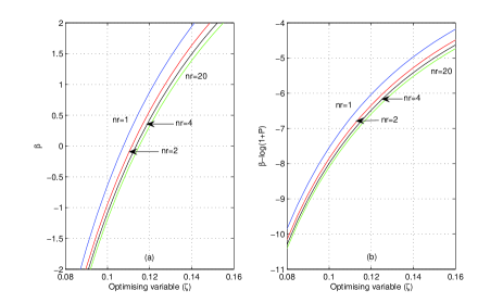
Figure 1: (a) The quantity $\beta$ in (15) as a function of $\zeta$ showing $\zeta$ which produce both negative and positive values for $\beta=\mathrm{E}_{x}\{\log(1+x^{2})\}$, SNR=30 dB. (b) Shows $\beta-\log(1+P)$ is an increasing function of $\zeta$.

The capacity $C(\zeta)$ is a monotonically decreasing function of $\zeta$ since

$$\frac{\partial{C(\zeta)}}{{\partial}{\zeta}}=-\zeta{\Psi_{1}(\zeta)},$$ (20)

where $\Psi_{n}(\cdot)$ is the $n^{th}$ derivative of $\Psi(\cdot)$ [17, page 253-255]. Fig. 2 depicts the channel capacity for $\zeta\,\in\,(0,1)$. The capacity can be computed for some $\beta=\beta^{\prime}$, seeking the optimal $\zeta$ which satisfies the input power constraint. Furthermore, $\beta$ in (15) is a monotonically increasing function of $\zeta$ where

$$\frac{\partial{\beta(\zeta)}}{{\partial}{\zeta}}=-\frac{1}{\zeta}+\Psi_{1}(\zeta).$$ (21)

Therefore, the supremum of (18)

$$C_{\text{sup}}=C(\zeta_{s})=G(\zeta_{s})-G(n_{r})$$ (22)

is obtained with $\beta=0$ where the corresponding $\zeta_{s}$ is given by

$$\Psi(\zeta_{s})-\log(\zeta_{s})=\Psi(n_{r})-\log\left[n_{r}(1+P)\right].$$ (23)

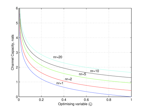
Figure 2: Channel capacity (18) as a function of $\zeta$, SNR=30dB.

.

The input power $P$ in (23) vs $\zeta_{s}$ as a function of $n_{r}$ is given in Fig. 3. It is clear that there exist $\zeta_{s}$ which gives the solution to (23) for any $P$ for a given $n_{r}$.

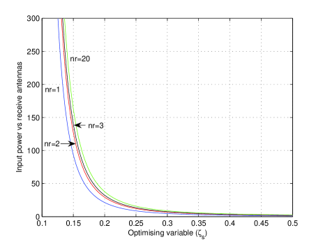
Figure 3: Input power (23) as a function of $\zeta_{s}$ showing the available solutions for $\zeta_{s}$ for any $P$, $n_{r}\,\in\,\{1,2,3,20\}$.

Fig. 4 shows the capacity supremum in (22) against the input power for different $n_{r}$ equating $\zeta_{s}$ in (23). This non-coherent Rayleigh fading MIMO channel capacity supremum can be used as an upper bound for all input distributions.

For larger $n_{r}$, Sengupta and Mitra [19] show the capacity of non-coherent Rayleigh fading MIMO channel

$$C_{\text{MIMO}}=\frac{1}{2}{\log\left(\frac{n_{r}}{{2}{\pi}}\right)}+\log{\mu}+\frac{P}{\mu{n_{t}}\left(1+\frac{P}{n_{t}}\right)}{\,\,,}$$ (24)

where

$$\mu=\int_{0}^{\infty}\frac{d{y}}{1+y}{\exp\left[{-\frac{y}{\mu\left(1+\frac{P}{n_{t}}\right)}}\right]}$$

and $\mu\approx\log(1+\frac{P}{n_{t}})$ for large $P$. Furthermore, they established a continuous input distribution which achieves (24) for large $n_{r}$. We will discuss the analysis of the capacity supremum in (22) with respect to (24) in Section V.

The capacity (22) is independent of the number of transmit antennas since the optimisation is carried out using magnitude of the input vector. Therefore, the effect of number of transmit antennas on capacity is not apparent. However, [9] proves that the capacity of $n_{t}\,>\,T$ is equal to the capacity for $n_{t}=T$ where $T$ is the channel coherence time. In this paper, we consider $T=1$, and therefore according to the theorem 1 in [9], the optimal $n_{t}=1$. Therefore, we conclude that capacity supremum (22) is true irrespective of $n_{t}$.

IV-D Optimal Input Distribution

The corresponding input distribution which provides this channel capacity supremum (22) for a certain $n_{r}$ is given by

$$\int_{0}^{\infty}{p_{X}(x)}{\frac{{y^{2{n_{r}}-1}}{\exp\left[{-{\frac{y^{2}}{2{(1+x^{2})}}}}\right]}}{{2^{n_{r}-1}}{\Gamma(n_{r})}{(1+x^{2})^{n_{r}}}}}{d{{x}}} =\frac{{{\zeta_{s}}^{\zeta_{s}}}{{y}^{{2}\zeta_{s}-1}}}{{{n_{r}}(1+P)^{\zeta_{s}}}{\Gamma(\zeta_{s})}}$$

$$\times\,{\exp\left[{-\frac{\zeta_{s}{{y}^{2}}}{2{n_{r}}(1+P)}}\right]}.$$ (25)

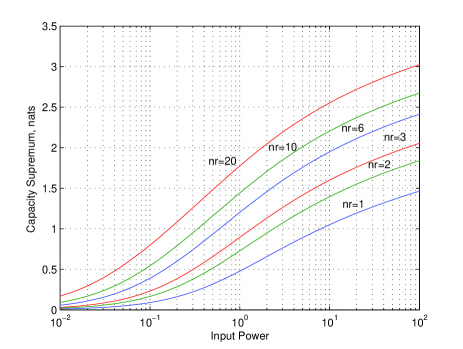
Figure 4: Capacity supremum (22) of the non-coherent Rayleigh fading MIMO channel with the input power for different number of receive antennas $n_{r}$.

The integral in (25) takes the form

$$\int_{a}^{b}K(s,t)f(t){dt}=g(s),$$ (26)

a well known Fredholm equation of the first kind [20] where $K(s,t)$ is the kernel. In general, such problems are ill-posed where small changes to the problem can make very large changes to the answer obtained. The kernel in (25) is analytic in $y$ over the whole plane for any $n_{r}$. However, the right hand side of (25) and its derivative with respect to $y$ is infinite when $y\,\rightarrow\,0$ for any $n_{r}$ and $\zeta_{s}$. Therefore, (25) does not provide a continuous solution for ${p_{X}(x)}$ in which the $C_{\text{sup}}$ in (22) is attained. This leads us to find a discrete input distribution in the form of

$${p_{X}(x)}=\sum_{i=1}^{N}{p_{i}}{\delta(x-x_{i})},$$ (27)

where $p_{i}$ and $x_{i}$ to be obtained solving

$$g(s)=\sum_{i=1}^{N}{p_{i}}{K(s,t_{i})}.$$ (28)

The number of transmitters $n_{t}$ has no effect on the result. The only requirement is to Euclidean norm of the input vector $\boldsymbol{X}$ be discrete irrespective of transmit diversity. For a discrete input, we can pose a new optimisation problem to compute the channel capacity

$$C_{\text{dis}} ={\text{sup}\atop{\Sigma_{i=1}^{N}p_{i}=1\atop{\Sigma_{i=1}^{N}p_{i}{x_{i}^{2}}\,\leq\,P}}}\int_{0}^{\infty}\int_{0}^{\infty}p_{X}(x){p_{Y|X}(y|x)}$$

$$\times\,\log\left[{\frac{p_{Y|X}(y|x)}{\int_{0}^{\infty}p_{X}(x){p_{Y|X}(y|x)}}}\right]{dy}{dx}$$

$$={\text{sup}\atop{\Sigma_{i=1}^{N}p_{i}=1\atop{\Sigma_{i=1}^{N}p_{i}{x_{i}^{2}}\,\leq\,P}}}\sum_{i=1}^{N}\int_{0}^{\infty}p_{i}{p_{Y|X}(y|x_{i})}$$

$$\times\,\log\left[{\frac{p_{Y|X}(y|x_{i})}{\sum_{j=1}^{N}p_{j}{p_{Y|X}(y|x_{j})}}}\right]{dy},$$ (29)

subject to the input power constraint $P$. If the solution exists for (IV-D), it will provide a good lower bound to $C_{\text{sup}}$. However, this optimisation problem is extremely difficult since the number of discrete points $N$ is unknown and the optimum probabilities and their locations to be found satisfying the input power constraint. Similar work is reported in [5] for a single antenna case and the numerical evaluation is given using the Kuhn Tucker conditions in order to verify the optimality of the capacity achieving mass point probabilities and their locations. Further work is required in this area to identify the optimal input at any SNR. The capacity supremum in (22) can be treated as an upper bound for the capacity of non-coherent Rayleigh fading MIMO channel.

IV-E Capacity for $\beta\,>\,0$

In addition to the capacity supremum found in the previous subsection, we now elaborate another solution when $\beta\,>\,0$ as the capacity for a MIMO system with a small number of receive antennas $n_{r}$. Since $\beta$ is an increasing function of $\zeta$ for a given $n_{r}$ we can obtain the capacity

$$C^{\prime}_{\text{sup}}(\alpha) =G(\alpha)-G(n_{r}),$$ (30)

for the input power

$$P=\frac{\alpha}{2{n_{r}}}{\exp\left[{{2}(\Psi(n_{r})+\log{2})-\Psi(\alpha)}\right]}-1,$$ (31)

when $\beta=\Psi(n_{r})+\log{2}\,>0$.

The quantity $\alpha\,\in\,(0,\infty)$, and the upper limit of $P$ is a function of $n_{r}$. For large $n_{r}$ and low input power there is no $\alpha$ which provides a solution to (31). This could be seen from the asymptotic value of (31)

$${P{{}_{\text{asy}}}}=\frac{1}{{2{n_{r}}}}{\exp\left[{2(\Psi(n_{r})+\log{2})}\right]}-1,$$ (32)

when $\alpha$ approaches infinity since the minimum $P$ is very high for $n_{r}\,\geq\,2$. Fig. 5 illustrates this, where there is no solution for $P=0$ in (31) when $n_{r}\,\geq\,2$.

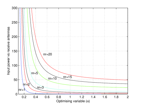
Figure 5: Input power (31) vs $\alpha$, showing that no solution exists when $P=0$ for $n_{r}\,\geq\,2$.

.

This excludes us in finding a solution to (30) for $n_{r}\,\geq\,2$. However, we can show the capacity in (30) for $n_{r}=1$ when the solution exists for $\alpha$ in the whole input range of $P$.

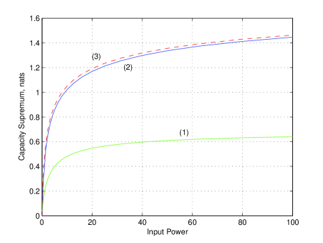
Figure 6: Comparison of capacities $C^{\prime}_{\text{sup}}$ and $C_{\text{sup}}$ for $n_{r}=1$. (1) Capacity of a SISO non-coherent Rayleigh fading channel with a discrete input [5]. (2) Capacity $C_{\text{sup}}$ when $\beta=0$ (3) Capacity $C^{\prime}_{\text{sup}}$ when $\beta=\Psi(n_{r})+\log{2}$.

For $n_{r}=1$, (22) and (23) becomes

$$C_{\text{sup}}(\zeta_{s})_{n_{r}=1}=(\alpha-\gamma-1)+\log{\Gamma(\zeta_{s})}-\zeta_{s}{\Psi(\zeta_{s})}$$ (33)

and

$$P{{}_{n_{r}=1}}=\zeta_{s}{e^{-\gamma-\Psi(\zeta_{s})}}-1$$ (34)

giving the capacity bound shown in [6, 21] for the non-coherent SISO Rayleigh fading channel.

A direct upper bound to both (22), (30) can be drawn since both relate to non-coherent capacity with channel coherent time $T=1$. The proven capacity is inherently less than the capacity with perfect CSI. Therefore we get

$$C^{\prime}_{\text{sup}}(\alpha)\,<\,C_{\text{rcsi}}\,\,\,,\,\,C_{\text{sup}}(\zeta_{s})\,<\,C_{\text{rcsi}}.$$ (35)

In [22], the sublinear behavior of MIMO channel capacity at low SNR is discussed. The two extremes, the capacity of channels with full and partial CSI is studied quantifying the maximum penalty for not having CSI at the receiver. It is shown that capacity loss due to unknown CSI increases monotonically with number of receive antennas, elaborating the significance of CSI at the receiver. Therefore, bounds shown in (35) become loose as $n_{r}$ increases.

IV-F Asymptotic Analysis

We consider the asymptotic analysis of the capacity supremum (22) when $P\,\rightarrow\,\infty$. $P$ in (23) approaches $\infty$ when $\zeta_{s}\,\rightarrow\,0$ since [17]

$${{\lim}\atop{{\zeta_{s}}_{\to}\,0}}\left({\frac{\zeta_{s}}{e^{\Psi(\zeta_{s})}}}\right)\,\rightarrow\,\infty.$$ (36)

Also when $\zeta_{s}=1$,

$$P=\frac{1}{{2}{n_{r}}}{\exp[\Psi(n_{r})+\log{2}+\gamma]}-1,$$ (37)

where the input power is zero for $n_{r}=1$ and a non-zero quantity for $n_{r}\,>\,1$. Therefore, $\zeta_{s}=1$ is not valid for $n_{r}\,>\,1$ and the $\zeta_{s}$ which produces $P=0$ can be found by solving

$$\log{\zeta_{s}}-\Psi(\zeta_{s})=\log({n_{r}})-\Psi(n_{r}),$$ (38)

for each $n_{r}$. We find an expression for $\zeta_{s}$, when $P$ approaches infinity, as a result of $\zeta_{s}$ approaching zero. From (23) we get

$$\log{\zeta_{s}} =\Psi(\zeta_{s})+\log{n_{r}}(1+P)-\Psi(n_{r}).$$ (39)

Multiplying the both sides of (39) by $\zeta_{s}$ and using

$${{\lim}\atop{{\zeta_{s}}_{\to}\,0}}\left({\zeta_{s}{\log{\zeta_{s}}}}\right)=0,$$

and

$${{\lim}\atop{{\zeta_{s}}_{\to}\,0}}\left({\zeta_{s}{\Psi(\zeta_{s})}}\right)=-1,$$

[17], we get

$$\zeta_{s}\,\approx\,\frac{1}{\log{n_{r}}(1+P)}.$$ (40)

Substituting $\zeta_{s}$ from (40) into (22) we get the asymptotic capacity

$$C_{\text{sup}}\approx\log[\log{n_{r}}(1+P)].$$ (41)

Note here the double logarithmic behavior of the asymptotic value, also depicted in [4, 6, 11, 19], for both the MIMO and SISO configurations. The effect of capacity at high SNR is extensively studied in [23] with the fading number

$$\mathcal{X}\triangleq\,{{\lim}\atop{{\text{SNR}}\to\,\infty}}\left\{{C(\text{SNR})-\log\log{\text{SNR}}}\right\},$$ (42)

and degrees of freedom defined by $n_{\text{min}}\triangleq\text{min}\{n_{t},n_{r}\}$. The asymptotic capacity

$$C(\text{SNR})=\log[1+\log(1+\text{SNR})]+\mathcal{X}+o(1),$$ (43)

indicates that at high SNR, capacity grows double logarithmically where the antenna numbers hardly influence the capacity. Our result further proves this argument since the effect of $n_{r}$ in (43) on capacity is negligible at high SNR.

V Numerical Results

For $n_{r}=1$, the numerical results obtained with $\beta=\Psi(n_{r})+\log{2}$ in Fig. 6 is slightly higher than $C_{\text{sup}}$ at any SNR. It is clear that $\beta=0$ provides the lowest upper bound as predicted in Section IV-C. However, for $n_{r}\,\geq\,2$, the bounds do not exist for any SNR as explained in Section IV-E. The solutions to (22) and (23) lead to good upper bounds for any $n_{r}$. Moreover, accurate bounds could be realised using these solutions even at high SNR where $\beta=0$.

The SISO channel capacity shown by Abou-Faycal [5] with a discrete input is included in Fig. 6. It is $\sim\,50\%$ lower than the capacity supremum. Also capacity increase having more antennas at the receiver is not promising at high SNR as in the coherent Rayleigh fading MIMO channel.

Furthermore, we compare the capacity supremum (22) with the results produced by Sengupta and Mitra in [19] for high $n_{r}$ at high $P$ with $n_{t}=1$. Fig. 7 depicts the comparison of the capacity supremum vs capacity (24) for $n_{r}\,\in\,\{10,20,30,50\}$ at high SNR. From the graph, it is clear that the gap between the capacities in (22) and (24) for a specific $n_{r}$ becomes small as the input power increases. The limit is shown in (41) for any $n_{r}$ illustrating the double logarithmic behavior at high SNR.

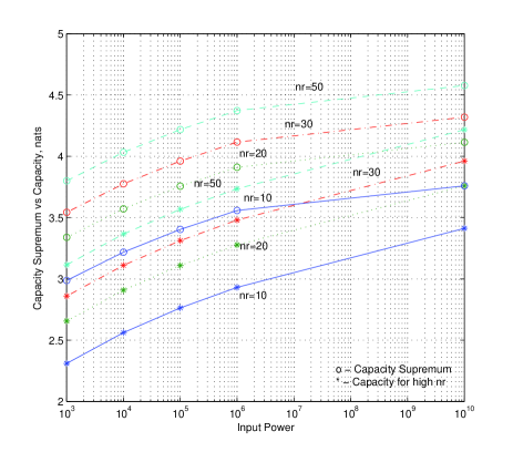
Figure 7: Capacity supremum in (22) “o”, vs the capacity for high $n_{r}$ given in (24) “*”, at high input power. Both the capacities approach the limit shown in (41) resulting the double logarithmic asymptotic behavior.

VI Conclusions

In this paper, we investigated the capacity of uncorrelated MIMO channels when neither the receiver nor the transmitter has the knowledge of CSI except its fading statistics. Capacity supremum is given in two cases, where one predicts accurate values for any number of receive antennas. The main findings of this paper is the capacity supremum for the non-coherent uncorrelated Rayleigh fading MIMO channel with no CSI for a given number of receiver antennas at any SNR.

We have shown the asymptotic behavior of the capacity supremum at high SNR. Furthermore, it is compared with the capacity shown in the literature having large number of receive antennas. Furthermore, the capacity supremum is shown to be independent of number of transmit antennas and increases with the number of receive antennas. The results of this paper can be used as an upper bound to the non-coherent uncorrelated Rayleigh fading MIMO channel with any input distribution.

The input distribution for the capacity upper bound is proven to be non-continuous. Hence the optimisation problem is posed for a discrete input with $N$ mass points. Capacity obtained from the discrete input with optimal number of mass points, probabilities and their locations will be a lower bound to the capacity supremum derived in this paper. The capacity increase with increasing number of receive antennas is not promising at high SNR as in the coherent channel. Therefore, channel estimation becomes more important as the number of antenna elements at the receiver is increased.

VII APPENDIX

VII-A Derivation of the constraint in (8c)

We use (4) in LHS of (8c) to write

$$\int_{0}^{\infty}{p_{Y}(y)}{\log{y}}{d{{y}}} =\int_{0}^{\infty}\int_{0}^{\infty}{p_{X}(x)}\left\{\frac{{y^{2{n_{r}}-1}}}{{2^{n_{r}-1}}{\Gamma(n_{r})}}\right.$$

$$\left.\times\,\frac{\exp\left[{-{\frac{y^{2}}{2{(1+x^{2})}}}}\right]}{{(1+x^{2})^{n_{r}}}}\right\}({\log{y}})\,{d{{y}}}{d{{x}}}.$$ (44)

Using the integral identity [16]:

$$\int_{0}^{\infty}{x^{t}}{e^{-{u{x}^{2}}}}{\log{x}}{dx} =\frac{u^{-\frac{t}{2}}}{4{\sqrt{u}}}{\Gamma\left(\frac{t+1}{2}\right)}$$

$$\times\,\left[\Psi\left({\frac{t+1}{2}}\right)-\log{u}\right],$$ (45)

we simplify (44) as

$$\int_{0}^{\infty}{p_{Y}(y)}{\log{y}}\,{d{{y}}} =\frac{1}{2}\int_{0}^{\infty}{p_{X}(x)}\left[\Psi(n_{r})\right.$$

$$\left.+\log{2}{(1+{x}^{2})}\right]{d{{x}}}$$

$$=\frac{1}{2}[\beta+\Psi(n_{r})+\log{2}].$$ (46)

This constraint is used in addition to the constrained input power in calculating the capacity supremum where $\beta=\mathrm{E}_{x}\{\log(1+x^{2})\}$.

VIII ACKNOWLEDGEMENTS

National ICT Australia (NICTA) is funded through the Australian Government’s Backing Australia’s Ability Initiative, in part through the Australian Research Council. The authors would like to thank Michael Williams for helpful discussions.

References

- [1] I. E. Telatar, “Capacity of multi-antenna Gaussian channels,” Tech. Repo., AT&T Bell Labs, 1995.
- [2] W. Chao, W.U. Sjunjun, Z. Linrang, and T. Xiaoyan, “Capacity evaluation of MIMO systems by Monte-Carlo methods,” IEEE International Conf. on Neural Networks and Signal Processing, pp. 1464–1466, Dec. 2003.
- [3] M. A. Khalighi, J. M. Brossier, G. Jourdain, and K. Raoof, “Water filling capacity of Rayleigh MIMO channels,” IEEE Journal on Selected Areas in Communications, vol. 01, pp. 155–158, Oct. 2001.
- [4] Y. Liang and V. V. Veeravalli, “Capacity of noncoherent time selective Rayleigh fading channels,” IEEE Trans. on Info. Theory, vol. 50, no. 12, pp. 3095–3110, Dec. 2004.
- [5] I. C. Abou-Faycal, M. D. Trott, and S. Shamai, “The capacity of discrete-time memoryless Rayleigh-fading channels,” IEEE Trans. on Info. Theory, vol. 47, no. 04, pp. 1290–1301, May 2001.
- [6] G. Taricco and M. Elia, “Capacity of fading channel with no side information,” IEE Electronics Letters, vol. 33, no. 16, pp. 1368–1370, July 1997.
- [7] J. Huang and S. Meyn, “Characterisation and computation of optimal distributions for channel coding,” in Proc. IEEE Trans. on Info. Theory, 2005.
- [8] J. G. Smith, “The information capacity of amplitude and variance-constrained scalar Gaussian channels,” Information and Control, vol. 18, pp. 203–219, 1971.
- [9] T. L. Marzetta and B. M. Hochwald, “Capacity of a mobile multiple-antenna communication link in Rayleigh flat fading,” IEEE Trans. on Info. Theory, vol. 45, no. 01, pp. 139–157, Jan. 1999.
- [10] L. Zheng and D. N. C. Tse, “Communication on the Grassmann manifold: A geometric approach to the noncoherent multiple-antenna channel,” IEEE Trans. on Info. Theory, vol. 48, no. 02, pp. 359–383, Feb. 2002.
- [11] A. Lapidoth and S. Moser, “On the fading number of multi-antenna systems over flat fading channels with memory and incomplete side information,” IEEE Int. Symp. on Info. Theory, vol. Lausanne, Switzerland, pp. 478–478, June-July 2002.
- [12] G. Foschini and M. Gans, “On limits of wireless communications in a fading environment when using multiple antennas,” Wireless Personal Communications, vol. 06, pp. 311–335, Mar. 1998.
- [13] A. J. Goldsmith and P. P. Varaiya, “Capacity of fading channels with channel side information,” IEEE Trans. on Info. Theory, vol. 43, no. 06, pp. 1986–1992, Nov. 1997.
- [14] R. G. Gallager, Information theory and reliable communication, John Wiley and Sons, USA, 1968.
- [15] S. Boyd and L. Vandenberghe, Convex Optimisation, Cambridge University Press, United Kingdom, 2004.
- [16] I. S. Gradshteyn and I. M. Ryzhik, Table of integrals, series, and products, Academic press San Diego, USA, sixth edition, 2000.
- [17] M. Abramowitz and I. A. Stegun, Handbook of Mathematical Functions, Dover Publications, Inc, New York, 1965.
- [18] T. M. Cover and J. A. Thomas, Elements of Information Theory, John Wiley, New York, 1991.
- [19] A. M. Sengupta and P. P. Mitra, “Capacity of multivariate channels with multiplicative noise,” Tech. Repo., AT&T Bell Labs, 2004.
- [20] L. M. Delves and J.L. Mohamed, Computational methods for integral equations, Cambridge University Press, Great Britain, 1985.
- [21] W. Zhang and J. N. Laneman, “An induced additive-noise model for non-coherent discrete-time memoryless Rayleigh fading channels,” Conference on Information Sciences and Systems, The Johns Hopkins University, March 16-18 2005.
- [22] S. Ray, M. Medard, L. Zheng, and J. Abounadi, “On the sublinear behavior of MIMO channel capacity at low SNR,” IEEE Int. Symp. on Info. Theory, pp. 1031–1034, Parma, Italy, Oct. 2004.
- [23] T. Koch and A. Lapidoth, “The fading number and degrees of freedom in non-coherent MIMO fading channels: A peace pipe,” IEEE Int. Symp. on Info. Theory, pp. 661–665, Adelaide, Australia, Sept. 2005.