A Decision Theoretic Framework for Real-Time Communication

Abstract

We consider a communication system in which the outputs of a Markov source are encoded and decoded in real-time by a finite memory receiver, and the distortion measure does not tolerate delays. The objective is to choose designs, i.e. real-time encoding, decoding and memory update strategies that minimize a total expected distortion measure. This is a dynamic team problem with non-classical information structure [7]. We use the structural results of [4] to develop a sequential decomposition for the finite and infinite horizon problems. Thus, we obtain a systematic methodology for the determination of jointly optimal encoding decoding and memory update strategies for real-time point-to-point communication systems.

Keywords: Real-time communication, finite-delay communication, zero-delay communication, joint source-channel coding, Markov decision theory

1 Introduction

Real-time communication problems arise in controlled decentralized systems where information must be exchanged between various nodes of the system and decisions based on the communicated information must be made in real-time. Such systems include QoS (delay) requirements and distributed routing in wired, wireless and sensor networks, traffic flow control in transportation networks, resource allocation and consensus in partially synchronous systems and decentralized resource allocation problems in economic systems.

We consider point-to-point real-time communication system as shown in Figure 1, which is the simplest system of this class. A better understanding of this case is needed before generalizing to multi-terminal systems. In the system under consideration, the outputs of a Markov source are encoded in real-time into a sequence of random variables. This sequence is transmitted through a discrete memoryless channel (DMC) to a receiver with finite memory. At each time instant $t$, using the current channel output and its current memory content, the receiver updates its memory and estimates the source output at $t$. The system designer has to choose real-time encoding, decoding and memory update rules that minimize an expected total distortion.

Real-time or finite-delay communication problems have been considered in the past. For an extensive literature survey we refer the reader to [4, 3]. Here we will only refer to the papers most relevant to our philosophy and approach. Real-time encoding and decoding with limited memory make the standard Information theoretic techniques inappropriate for this problem. Most of the results of Information theory are based on some form of the law of large numbers, which becomes applicable only when we consider sufficiently long sequences. This problem does not have enough structure to use encoding and decoding of typical sequences. Hence, we consider a decision theoretic approach to the problem.

Decision theoretic approaches to real-time communication similar in spirit to ours have appeared in [11, 1, 5, 2, 4]. Real-time communication problems for noiseless channel were studied in [11, 1]. Real-time encoding decoding problems for a noisy channel and noiseless feedback were studied in [5, 2]. These problems share a common feature that at every stage the encoder has perfect knowledge of the information available to the decoder/receiver. The case of a noisy channel and no feedback does not share this feature. Real-time communication through noisy channels and no feedback was investigated in [4] and structural results for optimal real-time encoding and decoding strategies were obtained. However, to the best of our knowledge, the problem of obtaining jointly optimal real-time encoders, decoders and memory update rules has not been considered by anyone so far. In this paper we present a methodology for this joint optimization. We present the key ideas and fundamental results here, and refer the reader to [3] for details and extensions.

The remainder of the paper is organized as follows. In Section 2 we formally define the problem, in Section 3 we restate the structural results of [4], in Section 4 we present the joint optimization of encoder, decoder and memory update. In Sections 5 and 6 we consider the finite and infinite horizon time homogeneous cases. We discuss some salient points in Section 7 and conclude in Section 8.

Notation: When using English letters to represent a variable, we use the standard notation of using uppercase letters ($X,Y,Z$) for denoting random variables and lowercase letters for denoting their realization ($x,y,z$). While representing a function of random variables as a random variable ($P_{M},P_{Y,M}$), we use a tilde above the variable to denote its realization ($\widetilde{P}_{M},\widetilde{P}_{Y,M}$). When using Greek letters to represent a random variable ($\pi,\varphi$), we use a tilde above the variable to denote its representation ($\tilde{\pi},\tilde{\varphi}$). We also use the standard short-hand notation of $x_{s}^{t}$ to represent the sequence $x_{s},\dots,x_{t}$ , $x_{1}^{t}$ is abbreviated to $x^{t}$ and similar notation for random variables and functions.

2 Problem Formulation

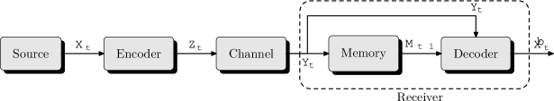
Figure 1: Real-Time Communication System

We now give a formal description of the problem under consideration. Consider a discrete time communication system shown in Figure 1. A first order Markov source produces a random sequence $X_{1},\dots,X_{T}$. For simplicity of exposition we assume that $X_{t}$ belongs to a finite alphabet $\mathcal{X}\triangleq\set{1,\dots,\left|\mathcal{X}\right|}$.

At each stage $t$, the encoder can transmit a symbol $Z_{t}$ taking values in a finite alphabet $\mathcal{Z}\triangleq\set{1,\dots,\left|\mathcal{Z}\right|}$. This encoded symbol must be generated in real-time, i.e.,

$$Z_{t}=c_{t}(X_{1},\dots,X_{t}),\qquad t=1,\dots,T,$$ (1)

and transmitted through a $\left|\mathcal{Z}\right|$-input $\left|\mathcal{Y}\right|$-output discrete memoryless channel producing the sequence $\set{Y_{1},\dots,Y_{T}}$, with each $Y_{t}$ belonging to an alphabet $\mathcal{Y}\triangleq\set{1,\dots,\left|\mathcal{Y}\right|}$. The transition probabilities of the channel is given by

$$\Pr\left({y_{t}|x^{t},z^{t},y^{t-1}}\right)=\Pr\left({y_{t}|z_{t}}\right)=P_{t}(y_{t},z_{t}).$$ (2)

At the receiver, the most that could be accessible at stage $t$ is the subsequence $Y_{1},\dots,Y_{t}$. However, we assume that the receiver has a memory of $\log_{2}\left|\mathcal{M}\right|$ bits. So, after some time, all the past observations can not be stored and the receiver must selectively shed information. We model this by assuming that the contents of the memory belong to a finite alphabet $\mathcal{M}\triangleq\set{1,\dots,\left|\mathcal{M}\right|}$. The memory is arbitrarily initialized with $M_{0}=1$ and then updated at each stage according to the rule

$$M_{t}=l_{t}(Y_{t},M_{t-1}),\qquad t=1,\dots,T-1.$$ (3)

The objective of the decoder is to generate an estimate of the source output in real-time. This estimate $\widehat{X}_{t}$ has to be generated from the present channel output $Y_{t}$ and the memory contents $M_{t-1}$, by some decoding rule, i.e.,

$$\widehat{X}_{t}=g_{t}(Y_{t},M_{t-1}),\qquad t=1,\dots,T.$$ (4)

The performance of the system is defined by way of a sequence of distortion functions. For each $t$, $\rho_{t}:\mathcal{X}\times\mathcal{X}\to[0,\infty).$ is given. Then, $\rho_{t}(X_{t},\widehat{X}_{t})$ measures the distortion at stage $t$.

A choice $(c,g,l)$ of decision rules for all stages is called a design, where $c\triangleq(c_{1},\dots,c_{T})$, $g\triangleq(g_{1},\dots,g_{T})$ and $l\triangleq(l_{1},\dots,l_{T-1})$. The performance of a design is quantified by the expected distortion under that design, which is given by

$$\mathcal{J}(c,g,l)\triangleq\mathds{E}\Set{\mathop{\mathord{\raise 0.49991pt\hbox{$\displaystyle\sum$}}}\slimits@_{t=1}^{T}\rho_{t}(X_{t},\widehat{X}_{t})}{c,g,l}.$$ (5)

The optimization problem that we consider is as follows:

Problem 1.

Assume that the encoder and the receiver know the statistics of the source (i.e. PMF of $X_{1}$ and the transition probabilities $P_{X_{t+1}|X_{t}}$), the channel transition matrix $P_{t}$, the distortion function $\rho_{t}(\cdot,\cdot)$ and a time horizon $T$. Choose a design $(c^{*},g^{*},l^{*})$ that is optimal with respect to the performance criterion of (5), i.e.,

$$\mathcal{J}(c^{*},g^{*},l^{*})=\mathcal{J}^{*}\triangleq\min_{\begin{subarray}{c}c\in\mathscr{C}^{T}\\ g\in\mathscr{G}^{T}\\ l\in\mathscr{L}^{T-1}\end{subarray}}\mathcal{J}(c,g,l),$$ (6)

where $\mathscr{C}^{T}\triangleq\mathscr{C}_{1}\times\dots\times\mathscr{C}_{T}$, where $\mathscr{C}_{t}$ is the family of functions from $\mathcal{X}^{t}\to\mathcal{Z}$, $\mathscr{G}^{T}\triangleq\mathscr{G}\times\dots\times\mathscr{G}$ ($T$-times), where $\mathscr{G}$ is the family of functions from $\mathcal{Y}\times\mathcal{M}\to\mathcal{X}$ and $\mathscr{L}^{T-1}\triangleq\mathscr{L}\times\dots\times\mathscr{L}$ ($(T-1)$-times), where $\mathscr{L}$ is the family of functions from $\mathcal{Y}\times\mathcal{M}\to\mathcal{M}$.

The problem belongs to the class of decentralized dynamic team problems with non-classical information structure. Such problems are difficult to solve as they are non-convex functional optimization problems. We can view the problem as a sequential stochastic optimization problem [8, 9] by a fictitious partitioning of stage $t$ into three parts. The encoder transmits at $t^{+}$, the decoder makes a decision at $(t+\frac{1}{2})$ and the memory is updated at $(t+1)^{-}$. Now we have a stochastic optimization problem with a horizon of $3T$ where the decision makers can be ordered in advance, thus the problem is sequential. Witsenhausen [8] presented a general framework to work with sequential stochastic optimization problems by converting them into standard form. The solution methodology presented therein is applicable only to finite horizon problems and can not be extended to infinite horizon problems. We exploit the structural results of [4] to obtain a solution methodology which can be extended to infinite horizon problems. For completeness of presentation we summarize the structural results of [4] next.

3 Structural Results

Definition 1.

Let $P_{M_{t}}$ be the encoder’s belief about the memory contents of the receiver, i.e.,

$$P_{M_{t}}(m)\triangleq\Pr\left({M_{t}=m|X^{t},Z^{t},c^{t},l^{t}}\right).$$ (7)

For a particular realization $x^{t}$ and an arbitrary (but fixed) choice of $c^{t}$, $l^{t}$, the realization of $P_{M_{t}}$ denoted by $\widetilde{P}_{M_{t}}$, is a PMF on $M_{t}$ and belongs to $\mathcal{P}^{\mathcal{M}}$, the space of PMFs on $\mathcal{M}$. If $X^{t}$ is random vector and $c^{t}$, $l^{t}$ are arbitrary (but fixed) functions, then $P_{M_{t}}$ is a random vector belonging to $\mathcal{P}^{\mathcal{M}}$.

Theorem 1 (Structure of Optimal Encoder).

Consider the problem of minimizing the expected distortion given by (5) for any arbitrary (but fixed) decoder $g$ and memory update $l$. Then, without loss in optimality, one can restrict attention to encoding rules of the form

$$Z_{t}=c_{t}(X_{t},P_{M_{t-1}}),\qquad t=2,\dots,T.$$ (8)

Theorem 2 (Structure of Optimal Decoder).

Consider the problem of minimizing the expected distortion given by (5) for any arbitrary (but fixed) encoder $c$ and memory update rule $l$. Then, the design of an optimal decoder is a filtering problem and an optimal decoding rule $g^{*}$ is given by

$$\hat{x}_{t} =g_{t}^{*}(y_{t},m_{t-1})=\tau_{t}\big{(}\xi_{t}(y_{t},m_{t-1})\big{)},$$ (9)

where

$$\xi_{t}(y,m)(x) =\Pr\left({X_{t}=x|Y_{t}=y,M_{t-1}=m}\right),$$ (10)

and

$$\tau_{t}(\xi_{t}) =\arg\min_{\hat{x}}\mathop{\mathord{\raise 0.49991pt\hbox{$\displaystyle\sum$}}}\slimits@_{x\in\mathcal{X}}\rho_{t}(x,\hat{x})\xi_{t}(x).$$ (11)

See [4] for a proof of these theorems.

3.1 Implication of Structural Results

The structural results simplify the problem as follows:

1. Theorem 1 implies that at each stage $t$, without loss in optimality, we can restrict attention to encoders belonging to $\mathscr{C}_{S}$, the family of functions from $\mathcal{X}\times\mathcal{P}^{\mathcal{M}}$ to $\mathcal{Z}$. Thus, at each stage, we can restrict to optimizing over a fixed (rather than time-varying) domain.

2. Theorem 2 implies that the structure of an optimal decoders is a deterministic function of $\rho_{t}$, the distortion measure at time $t$ and $\xi_{t}$, the conditional PMF at time $t$, which in turn depends only on the choice of decision rules $c^{t}$ and $l^{t-1}$. Thus, an optimal decoder at time $t$ can be written as $g^{*}_{t}=g^{*}_{t}(c^{t},l^{t-1})$, implying that an optimal decoder obtained by Theorem 2 can be expressed in terms of the encoder and memory update rule as $g^{*}(c,l)$. For any design define

   $$\widetilde{\mathcal{J}}(c,l)\triangleq\mathcal{J}\big{(}c,g^{*}(c,l),l\big{)},$$ (12)

   and consider the following problem:

   Problem 2.

   Under the assumptions of Problem 1, choose a design $(c^{*},l^{*})$ that is optimal with respect to the performance criterion of (12), i.e.,

   $$\widetilde{\mathcal{J}}(c^{*},l^{*})=\widetilde{\mathcal{J}}^{*}=\inf_{\begin{subarray}{c}c^{*}\in\mathscr{C}_{S}^{T}\\ l\in\mathscr{L}^{T}\end{subarray}}\mathcal{J}\big{(}c,g^{*}(c,l),l\big{)},$$ (13)

   where $\mathscr{C}_{S}^{T}\triangleq\mathscr{C}_{S}\times\dots\times\mathscr{C}_{S}$ ($T$-times)

   Clearly, $\widetilde{\mathcal{J}}^{*}=\mathcal{J}^{*}$ i.e., the design $(c^{*},g^{*},l^{*})$ obtained by an optimal solution $(c^{*},l^{*})$ of Problem 2, along with an optimal decoder $g^{*}(c^{*},l^{*})$ obtained by Theorem 2, is an optimal solution for Problem 1.

In the next section we provide a sequential decomposition for Problem 2.

4 Joint Optimization

The critical step in obtaining an optimization methodology based on sequential decomposition is identifying an information state sufficient for performance evaluation of the system. In this section, we give expressions for an information state and explain how to obtain a sequential decomposition of the problem. The intuition behind our approach is as follows. The distortion at stage $t$ depends on $X_{t}$ and $\widehat{X}_{t}$. We need to find a field basis and conditional basis for $\widehat{X}_{t}$ (see [7]) for each agent at each stage. However, just finding a field and conditional bases is not sufficient. These combined bases must form a state (in the sense of [10]) for the purpose of performance evaluation. Suppose $\pi_{t}$ and $\varphi_{t}$ are the information states of the encoder and memory update respectively. They need to satisfy the following properties:

1. $\pi_{t}$ is a function only of the encoder’s information and the past encoding and memory update rules. Any choice of the present encoding rule $c_{t}$ together with $\pi_{t}$ determine $\varphi_{t}$, the information state for the memory update at the next step.

2. $\varphi_{t}$ is a function only of the receiver’s information and the past encoding and memory update rules. Any choice of the present memory update rule $l_{t}$ together with $\varphi_{t}$ determine $\pi_{t+1}$, the information state for the encoder at the next step.

3. At each stage both the encoder and the receiver can evaluate the expected cost to go from their respective information state and choice of present and future decision rules. This expectation is conditionally independent of the past decision rules, conditioned on the current information state.

The above properties can be written more formally as follows:

(S1a)

$\pi_{t}$ is a function of $x^{t}$, $c^{t-1}$ and $l^{t-1}$.

(S1b)

$\varphi_{t}$ is a function of $y_{t}$, $m_{t-1}$, $c^{t}$ and $l^{t-1}$.

(S2a)

$\varphi_{t}$ can be determined from $\pi_{t}$ and $c_{t}$.

(S2b)

$\pi_{t+1}$ can be determined from $\varphi_{t}$ and $l_{t}$.

(S3)

For the purpose of performance evaluation, $\pi_{t}$ absorbs the effect of $c^{t-1},l^{t-1}$ and $\varphi_{t}$ absorbs the effect of $c^{t},l^{t-1}$ on expected future distortion, i.e.
$\mathds{E}\Set{\sum\limits_{s=t}^{T}\rho_{s}(X_{s},\widehat{X}_{s})}{c,g,l}=\mathds{E}\Set{\sum\limits_{s=t}^{T}\rho_{s}(X_{s},\widehat{X}_{s})}{\pi_{t},c_{t}^{T},l_{t}^{T}}$
$\hphantom{\mathds{E}\Set{\sum\limits_{t=s}^{T}\rho_{t}(X_{t},\widehat{X}_{t})}{c,g,l}}=\mathds{E}\Set{\sum\limits_{s=t}^{T}\rho_{s}(X_{s},\widehat{X}_{s})}{\varphi_{t},c_{t+1}^{T},l_{t}^{T}}$,
or alerntively

(S3^⋆)

$\mathds{E}\Set{\rho_{t}(X_{t},\widehat{X}_{t})}{c,g,l}=\mathds{E}\Set{\rho_{t}(X_{t},\widehat{X}_{t})}{\pi_{t},c_{t}}$
$\hphantom{\mathds{E}\Set{\rho_{t}(X_{t},\widehat{X}_{t})}{c,g,l}}=\mathds{E}\Set{\rho_{t}(X_{t},\widehat{X}_{t})}{\varphi_{t},l_{t}}.$

Properties (S1),(S2),(S3) are equivalent to properties (S1),(S2),(S3^⋆). (S1) and (S2) imply that $\pi_{t}$ and $\varphi_{t}$ are states and (S3) ensures that $\pi_{t}$ and $\varphi_{t}$ absorb the effect of past decision rules on expected future distortion. Thus, they are sufficient for the purpose of performance evaluation. In this section we find information states $\pi_{t}$ and $\varphi_{t}$ that satisfy (S1)–(S3). We define the following:

Definition 2.

Let $P_{Y_{t},M_{t-1}}$ be the encoder’s belief about the channel output and memory contents of the receiver, i.e.,

$$P_{Y_{t},M_{t-1}}(y,m)\triangleq\Pr\left({Y_{t}=y,M_{t-1}=m|X^{t},Z^{t},c^{t},l^{t-1}}\right).$$ (14)

For a particular realization $x^{t}$ and a particular choice $c^{t}$, $l^{t-1}$, the realization of $P_{Y_{t},M_{t-1}}$, denoted by $\widetilde{P}_{Y_{t},M_{t-1}}$, is a PMF on $(Y_{t},M_{t-1})$ and belongs to $\mathcal{P}^{\mathcal{Y}\times\mathcal{M}}$, the space of PMFs on $\mathcal{Y}\times\mathcal{M}$. If $X^{t}$ is a random vector and $c^{t}$, $l^{t-1}$ are arbitrary (but fixed) functions, then $P_{Y_{t},M_{t-1}}$ is a random vector belonging to $\mathcal{P}^{\mathcal{Y}\times\mathcal{M}}$.

Lemma 1.

At each stage $t$,

1. there is a deterministic function $\nu_{t}(\cdot)$ such that $P_{Y_{t},M_{t-1}}=\nu_{t}(P_{M_{t-1}},Z_{t}),$

2. there is a deterministic function $\psi_{t}(\cdot)$ such that $P_{M_{t}}=\psi_{t}(P_{Y_{t},M_{t-1}},l_{t}).$

Proof.

See [3]. ∎

Definition 3.

Let $\Pi$ (resp. $\Phi$) be the space of probability measures on $\mathcal{X}\times\mathcal{P}^{\mathcal{M}}$ (resp. $\mathcal{X}\times\mathcal{P}^{\mathcal{Y}\times\mathcal{M}}$). Define $\pi_{t}$ and $\varphi_{t}$ as follows:

$$\pi_{t} =\Pr\left({X_{t},P_{M_{t-1}}}\right),$$ (15)

$$\varphi_{t} =\Pr\left({X_{t},P_{Y_{t},M_{t-1}}}\right),$$ (16)

where $\pi_{t}$ (resp. $\varphi_{t}$) belongs to $\Pi$ (resp. $\Phi$).

Theorem 3.

$\pi_{t}$ and $\varphi_{t}$ are the information states for the encoder and memory update respectively, i.e.,

1. there is a linear transformation $Q_{t}(c_{t})$ such that

   $$\varphi_{t}=Q_{t}(c_{t})\pi_{t},$$ (17)

2. there is a linear transformation $\widehat{Q}_{t}(l_{t})$ such that

   $$\pi_{t+1}=\widehat{Q}_{t}(l_{t})\varphi_{t},$$ (18)

3. for any choice of $c$ and $l$, the expected conditional instantaneous cost can be expressed as

   $$\mathds{E}\Set{\rho_{t}(X_{t},\widehat{X}_{t})}{c^{t},g_{t}^{*}(c^{t},l^{t-1}),l^{t-1}}=\tilde{\rho}_{t}(\varphi_{t}).$$ (19)

   where $g^{*}_{t}(c^{t},l^{t-1})$ is an optimal decoding rule corresponding to $c^{t}$, $l^{t-1}$ and $\tilde{\rho}_{t}(\cdot)$ is a deterministic function.

Proof.

This follows from Lemma 1. See [3] for detailed proof. ∎

The choice of functions $c^{t}$, $l^{t-1}$, $g^{*}_{t}(c^{t},l^{t-1})$ make the variable $\widehat{X}_{t}$ a random variable with well defined distribution. Thus, the performance criterion of (12) can be rewritten as

$$\begin{split}\mathds{E}\Set{\sum_{t=1}^{T}\rho_{t}(X_{t},\widehat{X}_{t})}{c,g^{*}(c,l),l}&=\sum_{t=1}^{T}\mathds{E}\Set{\rho_{t}(X_{t},\widehat{X}_{t})}{c^{t},g_{t}^{*}(c^{t},l^{t-1}),l^{t-1}}\\ &=\mathop{\mathord{\raise 0.49991pt\hbox{$\displaystyle\sum$}}}\slimits@_{t=1}^{T}\tilde{\rho}_{t}(\varphi_{t}).\end{split}$$ (20)

Notice that (17) and (18) imply that $\pi_{t}$ and $\varphi_{t}$ are states, i.e. they satisfy (S1) and (S2). Moreover, (19) and (20) imply that $\pi_{t}$ and $\varphi_{t}$ are sufficient for performance evaluation, i.e., satisfy (S3). Hence Theorem 3 implies that Problem 2 is equivalent to the following deterministic optimization problem:

Problem 3.

Consider a deterministic system which evolves as follows:

$$\varphi_{t} =Q_{t}(c_{t})\pi_{t}, \qquad t =1,\dots,T,$$ (21)

$$\pi_{t+1} =\widehat{Q}_{t}(l_{t})\varphi_{t}, \qquad t =1,\dots,T-1,$$ (22)

where $c_{t}$ and $l_{t}$ are functions belonging to $\mathscr{C}_{s}$ and $\mathscr{L}$ respectively and $Q_{t}(\cdot)$ and $\widehat{Q}_{t}(\cdot)$ are deterministic transforms depending on $c_{t}$ and $l_{t}$ respectively. The initial state $\pi_{1}$ of the system is known. If the system is in state $\varphi$ at stage $t$, it incurs a cost $\tilde{\rho}_{t}(\varphi)$.

The optimization problem is to obtain decision rules $c\triangleq(c_{1},\dots,c_{T})$, $l\triangleq(l_{1},\dots,l_{T-1})$ to minimize the total cost over horizon $T$, i.e., find optimal design $(c^{*},l^{*})$ such that

$$\widetilde{\mathcal{J}}(c^{*},l^{*})=\widetilde{\mathcal{J}}^{*}=\inf_{\begin{subarray}{c}c^{*}\in\mathscr{C}_{S}^{T}\\ l^{*}\in\mathscr{L}^{T}\end{subarray}}\mathop{\mathord{\raise 0.49991pt\hbox{$\displaystyle\sum$}}}\slimits@_{t=1}^{T}\tilde{\rho}_{t}(\varphi_{t}).$$ (23)

This is a classical deterministic control problem; optimal functions $(c^{*},l^{*})$ are determined by the nested optimality equations given below.

Theorem 4.

An optimal design $(c^{*},l^{*})$ for Problem 3 (and consequently for Problem 2 and thereby for Problem 1) can be determined by the solution of the following nested optimality equations:

$$\widehat{V}_{T}(\varphi) \equiv 0,$$ (24)

$$V_{t}(\pi_{t}) =\inf_{c_{t}\in\mathscr{C}_{S}}\Big{[}\tilde{\rho}_{t}\big{(}Q_{t}(c_{t})\pi\big{)}+\widehat{V}_{t}\big{(}Q_{t}(c_{t})\pi\big{)}\Big{]}, t =1,\dots,T,$$ (25)

$$\widehat{V}_{t}(\varphi) =\min_{l_{t}\in\mathscr{L}}\Big{[}V_{t+1}\big{(}\widehat{Q}_{t}(l_{t})\varphi\big{)}\Big{]}, t =1,\dots,T-1.$$ (26)

Proof.

This is a standard result, see [6, Chapter 2] ∎

5 Time Homogeneous System — Finite Horizon Case

For many applications the system is time-homogeneous, that is, the source is time-invariant Markov process ($P_{X_{t+1}|X_{t}}$ does not depend on $t$), the channel is time-invariant (transition matrix $P_{t}$ does not depend on $t$) and the distortion metric $\rho_{t}(\cdot)$ is time invariant. For such a system, the functions $\nu_{t}(\cdot)$, $\psi_{t}(\cdot)$, the linear transforms $Q_{t}(\cdot)$, $\widehat{Q}_{t}(\cdot)$ and the distortion $\tilde{\rho}_{t}(\cdot)$ defined in Theorem 3 are time-invariant, so we can drop the subscripts $t$ and simply refer them as $\nu(\cdot)$, $\psi(\cdot)$, $Q(\cdot)$, $\widehat{Q}(\cdot)$ and $\tilde{\rho}(\cdot)$ respectively. So, we obtain an equivalent of Theorem 3 making the corresponding changes. Thus, Problem 3 reduces to a time-homogeneous problem — one in which state space, action space, system update equation and instantaneous cost do not depend on time. Hence the optimality equations of Theorem 3 can be written in a more compact manner We can define the following:

Definition 4.

Let $\mathcal{V}$ (resp. $\widehat{\mathcal{V}}$) be the family of functions from $\Pi$ (resp. $\Phi$) to $\mathds{R}^{+}$. Define operators $W(c)$ (resp. $\widehat{W}(l)$) from $\widehat{\mathcal{V}}$ to $\mathcal{V}$ (resp. $\mathcal{V}$ to $\widehat{\mathcal{V}}$) as follows:

$$\big{(}W(c)\widehat{V}\big{)}(\pi) =\tilde{\rho}\big{(}Q(c)\pi\big{)}+\widehat{V}\big{(}Q(c)\pi\big{)},$$ (27)

$$\big{(}\widehat{W}(l)V\big{)}(\varphi) =V\big{(}\widehat{Q}(l)\varphi\big{)}.$$ (28)

Further define transformations $\mathcal{W}$ (resp. $\widehat{\mathcal{W}}$) from $\widehat{\mathcal{V}}$ to $\mathcal{V}$ (resp. $\mathcal{V}$ to $\widehat{\mathcal{V}}$) as follows:

$$\big{(}\mathcal{W}\widehat{V}\big{)}(\pi) =\inf_{c\in\mathscr{C}_{S}}\big{(}W(c)\widehat{V}\big{)}(\pi),$$ (29)

$$\big{(}\widehat{\mathcal{W}}V\big{)}(\varphi) =\inf_{l\in\mathscr{L}}\big{(}\widehat{W}(l)V\big{)}(\varphi).$$ (30)

Theorem 5.

For the time-homogeneous case, the value functions $V_{t}$ and $\widehat{V}_{t}$ of Theorem 4 evolve in a time-homogeneous manner as follows:

$$\widehat{V}_{t} =\widehat{\mathcal{W}}V_{t+1}, \qquad t =1,\dots,T-1,$$ (31)

$$V_{t} =\mathcal{W}\widehat{V}_{t}, \qquad t =1,\dots,T,$$ (32)

with the terminal condition given by

$$\widehat{V}_{T}\equiv 0.$$ (33)

The arguments minimizing $V_{t}$ and $\widehat{V}_{t}$ at each stage determine the decision rules $c_{t}$ and $l_{t}$.

Proof.

This follows immediately from Theorem 4. ∎

6 Time Homogeneous System — Infinite Horizon Case

We consider a time-homogeneous system as in Section 5. However, instead of a finite horizon $T$, we consider the infinite horizon case with performance of a design determined by

$$\mathcal{J}(c,g,l)=\mathds{E}\Set{\sum_{t=1}^{\infty}\beta^{t-1}\rho(X_{t},\widehat{X}_{t})}{c,g,l},$$ (34)

where $\beta\in(0,1)$ is called the discount factor. With a slight modification of the proof of [4, Section 2.4] one can show that the structural results of Section 3 are also valid in this case. Further, Theorem 3 (with the changes mentioned in previous section) holds for the infinite-horizon case also.

Definition 5.

Define operators $W$, $\widehat{W}$ and transforms $\mathcal{W}$, $\widehat{\mathcal{W}}$ as in Definition 4, with one change — modify the definition of $W$ to take the discounting into account as follows:

$$\big{(}W(c)\widehat{V}\big{)}(\pi)=\tilde{\rho}\big{(}Q(c)\pi\big{)}+\beta\widehat{V}\big{(}Q(c)\pi\big{)}.$$ (35)

Theorem 6.

For the infinite horizon time-homogeneous system with the performance criterion of (34), the evolution of value function is governed by the following set of equations

$$V_{t} =\mathcal{W}\widehat{V}_{t},$$ (36)

$$\widehat{V}_{t} =\widehat{\mathcal{W}}V_{t+1}.$$ (37)

The arguments that minimize $\widehat{V}_{t}$ and $V_{t+1}$ at each stage determine the decision rules $c_{t}$ and $l_{t}$.

Proof.

This is the solution of the time-homogeneous problem formulated by considering a time-homogeneous version of Problem 3 with the optimization criteria being minimizing $\mathds{E}\Set{\sum_{t=1}^{\infty}\beta^{t-1}\tilde{\rho}(\varphi_{t})}{c,g^{*}(c,l),l}$. ∎

Definition 6.

A design $(c,l)$, $c\triangleq(c_{1},c_{2},\dots)$, $l\triangleq(l_{1},l_{2},\dots)$ is called stationary (or time-invariant) if $c_{1}\equiv c_{2}\equiv\dots\equiv c$, $l_{1}\equiv l_{2}\equiv\dots\equiv l$.

Theorem 7.

For the time homogeneous case with the performance measure of (34), if the distortion measure $\rho(\cdot)$ is bounded and discount factor $\beta<1$, then stationary designs are $\varepsilon$-optimal, that is, for any design $(c^{\prime},l^{\prime})$ and any $\varepsilon>0$, there exists a stationary design $(c^{\infty},l^{\infty})$ such that

$$\mathcal{J}(c^{\infty},l^{\infty})=V(\pi_{1})\leq\mathcal{J}(c^{\prime},l^{\prime})+\varepsilon,$$ (38)

where $V$ is the unique fixed point of

$$V=(\mathcal{W}\circ\widehat{\mathcal{W}})V,$$ (39)

and $c$ and $l$ are the corresponding $\arg\min$ and $c^{\infty}=(c,c,\dots)$, $l^{\infty}=(l,l,\dots)$.

Proof.

See [3]. ∎

We have shown that a unique stationary $\varepsilon$-optimal policy exists. Thus, for the infinite horizon problem, without loss of optimality, we can restrict attention to stationary policies. This simplifies the implementation of an optimal policy.

7 Discussion

It was shown in [8] that all sequential problems can be transformed to a standard form by moving all the uncertainty to the first stage and at each stage augmenting the state variable to carry all the information needed to determine the cost. Further an optimal policy for a problem in standard form can be obtained by solving a deterministic optimization problem. We believe that our methodology has a similar spirit as Witsenhausen’s standard form. We have a decentralized optimization problem that is sequential and an optimal design is obtained by the solution of a deterministic optimization problem. In our solution the state space is not increasing with time and allows us to use our approach to infinite horizon problems while the standard form is applicable only to finite horizon problems. The structural results of [4] are critical to our approach as they allow us to obtain an information state whose dimensionality does not change with time.

8 Conclusion

We have developed a methodology for the determination of jointly optimal real-time encoding, decoding and memory update strategies for point-to-point communication system. This methodology has been extended to $k$-th oder Markov sources, distortion metric accepting a finite delay of $\delta$ units and channels with memory (see [3] for details). We believe that the same methodology can be used for the determination of jointly optimal real-time encoding, decoding and memory update strategies for more complex communication systems.

References

- [1] V. Borkar, S. Mitter, and S. Tatikonda, “Optimal sequential vector quantization of Markov sources,” SIAM Journal of Optimal Control, vol. 40, no. 1, pp. 135–148, Jan 2001.
- [2] R. Lipster and A. Shiryayev, Statistics of Random Processes, Vol. II:Applications. Springer-Verlag, 1977.
- [3] A. Mahajan and D. Teneketzis, “On jointly optimal encoding, decoding and memory update for noisy real-time communication systems,” Department of EECS, University of Michigan, Ann Arbor, MI–48109-2122, Control Group Report CGR-05-07, Oct. 2005, to be submitted to IEEE Trans. on Information Theory.
- [4] D. Teneketzis, “On the structure of optimal real-time encoders and decoders in noisy communiation,” submitted for publication in IEEE Trans. on Information Theory.
- [5] J. C. Walrand and P. Varaiya, “Optimal causal coding—decoding problems,” IEEE Transactions on Information Theory, vol. 29, no. 6, pp. 814–820, Nov. 1983.
- [6] P. Whittle, Optimization Over Time, ser. Wiley series in Probability and Mathematical Statistics. John Wiley and Sons, 1982, vol. 1.
- [7] H. S. Witsenhausen, “Separation of estimation and control for discrete time systems,” Proceedings of the IEEE, vol. 59, no. 11, pp. 1557–1566, Nov. 1971.
- [8] ——, “A standard form for sequential stochastic control.” Mathematical Systems Theory, vol. 7, no. 1, pp. 5–11, 1973.
- [9] ——, “The instrinsic model for stochastic control: Some open problems,” in Lecture Notes in Economics and Mathematical Systems, 107. Springer Verlag, 1975, pp. 322–335.
- [10] ——, “Some remark on the concept of state,” in Directions in Large-Scale Systems, Y. Ho and S. Mitter, Eds. Plenum, 1976, pp. 69–75.
- [11] ——, “On the structure of real-time source coders,” Bell System Technical Journal, vol. 58, no. 6, pp. 1437–1451, July-August 1978.